Wannier functions and exchange integrals: The example of LiCu₂O₂

Abstract

Starting from a single band Hubbard model in the Wannier function basis, we revisit the problem of the ligand contribution to exchange and derive explicit formulae for the exchange integrals in metal oxide compounds in terms of atomic parameters that can be calculated with constrained LDA and LDA+U. The analysis is applied to the investigation of the isotropic exchange interactions of LiCu₂O₂, a compound where the Cu-O-Cu angle of the dominant exchange path is close to 90^∘. Our results show that the magnetic moments are localized in Wannier orbitals which have strong contribution from oxygen atomic orbitals, leading to exchange integrals that considerably differ from the estimates based on kinetic exchange only. Using LSDA+U approach, we also perform a direct ab-initio determination of the exchange integrals LiCu₂O₂. The results agree well with those obtained from the Wannier function approach, a clear indication that this modelization captures the essential physics of exchange. A comparison with experimental results is also included, with the conclusion that a very precise determination of the Wannier function is crucial to reach quantitative estimates.

I Introduction

In order to explain the homeopolar chemical bond in the hydrogen molecule, Heitler and London Heitler have derived the direct and exchange Coulomb integrals which can be written in the following form:

$$U=\int\frac{\phi^{*}_{i}(x)\phi_{i}(x)\phi^{*}_{i}(x^{\prime})\phi_{i}(x^{\prime})}{|x-x^{\prime}|}dxdx^{\prime}$$ (1)

and

$$J^{Coulomb}_{ij}=\int\frac{\phi^{*}_{i}(x)\phi_{j}(x)\phi^{*}_{j}(x^{\prime})\phi_{i}(x^{\prime})}{|x-x^{\prime}|}dxdx^{\prime},$$ (2)

where i and j are site indexes, and $\phi_{i}(x)$ is a wave function centered at the lattice site i. Taking into account the exchange Coulomb integral allows one to obtain bonding ($E=U-J^{Coulomb}_{ij}$) as well as antibonding ($E^{\prime}=U+J^{Coulomb}_{ij}$) states of H₂. Heitler and London have shown that the properties of the hydrogen molecule can be described correctly using these combinations of wave functions.

Then, in 1928, Heisenberg Heisenberg has used the exchange Coulomb integral $J^{Coulomb}_{ij}$ to explain ferromagnetism. Heisenberg has supposed that this exchange Coulomb integral corresponds to the exchange coupling in a spin model defined by the Hamiltonian:

$$H=\sum_{ij}J_{ij}\vec{S}_{i}\cdot\vec{S}_{j},$$ (3)

and that it is the main source of ferromagnetism in 3d metal compounds. However, if $\phi_{i}(x)$ in Eq.(1) is the atomic wave function centered on the $ith$ atom, then the overlap between wave functions on neighboring atoms is negligibly small. Therefore the exchange interaction derived through Eq.(2) can be neglected.

In 1959, P.W. Anderson Anderson has suggested a new type of exchange interaction process based on hopping (kinetic exchange interaction). In the context of the Hubbard model, Hubbard

$$H=\sum_{ij\sigma}t_{ij}a^{+}_{i\sigma}a_{j\sigma}+\frac{U}{2}\sum_{i\sigma}n_{i\sigma}n_{i-\sigma},$$ (4)

this exchange interaction can be expressed as $J^{kin}_{ij}=\frac{2t_{ij}^{2}}{U}$. This estimation of exchange interaction through hopping integrals is convenient and now widely used in the literature. However, if $J^{kin}_{ij}$ is small enough, other sources of exchange coupling become important. Indeed, the proper way to discuss exchange is to consider the basis of Wannier functions $W_{i}$ (where $i$ is the composite index of band and site) proposed by Wannier wannier in 1937 and defined as the Fourier transforms of a certain linear combination of Bloch functions $\psi_{nk}$ ($n$ is the band index and $k$ is the wave-vector in reciprocal space). In contrast to atomic wave functions $\phi_{i}(x)$, which are localized on one atom, the Wannier functions $W_{i}(x)$ are more extended in space and can be expressed through linear combination atomic wave functions, $W_{i}(x)=\sum_{jT}\alpha^{i}_{j}\phi_{j}(x-T)$ (where $\alpha^{i}_{j}$ is the contribution of the jth atomic orbital to Wannier function $W_{i}(x)$ and $T$ is a translation vector). The Wannier functions are the most localized ones within the subspace of low-energy excitations, which facilitates a direct physical interpretation consistent with interacting localized spins. Therefore, to use Wannier states instead of atomic sets is physically motivated. In particular, as we shall see, $J^{Coulomb}_{ij}$ defined in the Wannier basis plays a crucial role in the description of exchange interactions between magnetic moments in the case of nearly 90^∘ metal-oxygen-metal bonds.

These questions have already been discussed in several context in the literature. For instance, the authors of Ref. Kahn, have discussed two alternative ways, natural or orthogonalized magnetic orbitals, to describe the exchange interactions. They have concluded that the orthogonalized magnetic orbital approach clearly leads to simpler calculations and thus may be more appropriate for quantitative computations.

The competition between kinetic ($J^{kin}_{ij}$) and potential ($J^{Coulomb}_{ij}$) contributions to the total exchange interaction has been considered before in many works. In Ref. Graaf, , the authors have performed model calculations of a Cu₂O₆Li₄ cluster for different Cu-O-Cu angles. Their computational experiments have shown that the nearest-neighbor interaction reaches a maximum around 97^∘ and remains ferromagnetic up to angles as large as 104^∘. They have also concluded that the simple superexchange relation cannot be applied to Li₂CuO₂. In Ref. Pickett, , it was shown that unusual insulating ferromagnetism in La₄Ba₂Cu₂O₁₀ can be explained by intersite ferromagnetic ”direct exchange” (in our notation $J^{Coulomb}_{ij}$). The authors have concluded that the latter process occurs mainly at La and O sites and overwhelms the AF superexchange J${}^{kin}_{ij}$. The value of J${}^{Coulomb}_{ij}$ was calculated through a direct integration over the wave functions.

In the present paper, we revisit this issue in the context of constrained LDA and LSDA+U ab-initio approaches. The problem we want to address can be formulated as follows. In favourable situations, the exchange integrals calculated using LSDA+U agree quite well with the standard superexchange expression $J^{kin}_{ij}=\frac{2t_{ij}^{2}}{U}$ if the parameters $t_{ij}$ and $U$ are themselves determined from constrained LDA and LSDA+U. Such an interpretation of the LSDA+U results is a well accepted criterion to test the reliability of the result. But the standard superexchange expression $J^{kin}_{ij}=\frac{2t_{ij}^{2}}{U}$ often fails quantitatively, and even sometimes qualitatively, to reproduce the LSDA+U results. The main goal of this paper is to provide for such cases a generalization of the superexchange expression which is entirely expressed in terms of parameters that can be determined by constrained LDA and LSAD+U, and which can be used as an interpretation and an independent check of the LSDA+U results.

To this end, we start from the standard Hamiltonian in Wannier function basis for nearly 90^∘ metal-oxygen-metal bond. We show how the different Coulomb interaction terms of this Hamiltonian are related to parameters defined in the atomic basis set, with emphasis on the intraatomic exchange interaction of oxygen, J${}_{p}^{H}$, to which $J^{Coulomb}_{ij}$ is proportional when neighboring Wannier orbitals overlap on the oxygen atoms. We then present a simple expression for the exchange interactions between magnetic moments in the system. The parameters that enter this expression can themselves be estimated through LDA and LSDA+U calculations. This formalism is applied to the investigation of the magnetic properties of LiCu₂O₂, and the results are compared to those of first-principle LSDA+U approach.

The paper is organized as follows. In Section II, we discuss the Hubbard model in Wannier function basis. In Section III A, we shortly describe the crystal structure of LiCu₂O₂ and present the results of LDA calculation. In Section III B, we present the results of LSDA+U calculations and discuss the exchange interactions obtained between different pairs of magnetic moments in LiCu₂O₂. In Section IV, we briefly summarize our results.

II Hubbard model in Wannier function basis

The general Hamiltonian in Wannier function basis $W_{i}(x)$ can be written in the following form: Hubbard

$$H=\sum_{i,j,\sigma}t_{ij}a^{+}_{i\sigma}a_{j\sigma}+\frac{1}{2}\sum_{ijkl,\sigma\sigma^{\prime}}(ij|U|kl)a^{+}_{i\sigma}a^{+}_{j\sigma^{\prime}}a_{l\sigma^{\prime}}a_{k\sigma},$$ (5)

where

$$t_{ij}=\int W^{*}_{i}(x)\nabla^{2}W_{j}(x)dx$$

and

$$(ij|U|kl)=\int\frac{W^{*}_{i}(x)W_{k}(x)W^{*}_{j}(x^{\prime})W_{l}(x^{\prime})}{|x-x^{\prime}|}dxdx^{\prime}.$$

We analyze the complex Hamiltonian of Eq.(5) in the context of a 3-site model (see Fig.1) with nearly 90^∘ bonds and define two Wannier orbitals $W_{1}=\alpha\phi_{1}+\beta\phi_{p_{1}}$ and $W_{2}=\alpha\phi_{2}+\beta\phi_{p_{2}}$, which are constructed from the atomic wave functions: $\phi_{1}$, $\phi_{2}$, $\phi_{p_{1}}$ and $\phi_{p_{2}}$ (see Fig.1).

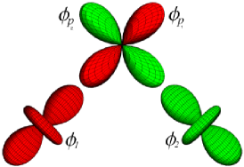
Figure 1: (Color online) Schematic representation of a nearly 90^∘ bond between 3d atoms through oxygen.

The oxygen orbitals $\phi_{p_{1}}$ and $\phi_{p_{2}}$ can be expressed through the angle of metal-oxygen-metal bond $\theta$ in the following form:

$$\phi_{p_{1}}=\cos(\frac{\theta-90^{\circ}}{2})\phi_{p_{y}}+\sin(\frac{\theta-90^{\circ}}{2})\phi_{p_{x}}$$ (6)

and

$$\phi_{p_{2}}=\cos(\frac{\theta-90^{\circ}}{2})\phi_{p_{x}}+\sin(\frac{\theta-90^{\circ}}{2})\phi_{p_{y}}.$$ (7)

Let us first analyze the hopping term in Eq.(5). It is easy to show that

$$t_{12}=\int W^{*}_{1}(x)\nabla^{2}W_{2}(x)dx=\beta^{2}\int\phi^{*}_{p_{1}}(x)\nabla^{2}\phi_{p_{2}}(x)dx.$$ (8)

If $\phi_{p_{1}}$ and $\phi_{p_{2}}$ are eigenfunctions of the Hamiltonian of Eq.(5), then using the orthogonality condition, one can obtain the following expression for the hopping term:

$$t_{12}\sim\beta^{2}\cos\theta.$$ (9)

Clearly, if $\theta=90^{\circ}$, the hopping integral vanishes.

In the analysis of the Coulomb term of Eq.(5) that follows, we consider only density-density terms and on-site exchange integrals. On-site Coulomb interaction, intersite Coulomb interaction and intersite exchange interaction in Wannier function basis are expressed through the corresponding parameters in the atomic basis set:

$$(ii|U|ii)=\alpha^{4}U_{d}+2\alpha^{2}\beta^{2}V_{pd}+\beta^{4}U_{p},\quad\quad\quad\quad\quad\quad$$ (10)

$$(ij|U|ij)=\alpha^{4}V_{dd}+2\alpha^{2}\beta^{2}V_{pd}+\beta^{4}U_{p},\quad\quad\quad\quad\quad\quad$$ (11)

$$(ij|U|ji)=\beta^{4}J^{H}_{p}\quad\quad\quad\quad\quad\quad\quad\quad\quad\quad\quad\quad\quad\quad$$ (12)

where

$$U_{d}=\int\frac{\phi^{*}_{1}(x)\phi_{1}(x)\phi^{*}_{1}(x^{\prime})\phi_{1}(x^{\prime})}{|x-x^{\prime}|}dxdx^{\prime}$$ (13)

is the on-site Coulomb interaction of 3d atom,

$$U_{p}=\int\frac{\phi^{*}_{p_{1}}(x)\phi_{p_{1}}(x)\phi^{*}_{p_{2}}(x^{\prime})\phi_{p_{2}}(x^{\prime})}{|x-x^{\prime}|}dxdx^{\prime}$$ (14)

is the on-site Coulomb interaction of oxygen atom,

$$V_{pd}=\int\frac{\phi^{*}_{1}(x)\phi_{1}(x)\phi^{*}_{p_{1}}(x^{\prime})\phi_{p_{1}}(x^{\prime})}{|x-x^{\prime}|}dxdx^{\prime}$$ (15)

is the Coulomb interaction between 3d atom and oxygen,

$$V_{dd}=\int\frac{\phi^{*}_{1}(x)\phi_{1}(x)\phi^{*}_{2}(x^{\prime})\phi_{2}(x^{\prime})}{|x-x^{\prime}|}dxdx^{\prime}$$ (16)

is the Coulomb interaction between 3d atoms,

$$J^{H}_{p}=\int\frac{\phi^{*}_{p_{1}}(x)\phi_{p_{2}}(x)\phi^{*}_{p_{2}}(x^{\prime})\phi_{p_{1}}(x^{\prime})}{|x-x^{\prime}|}dxdx^{\prime}$$ (17)

is the intraatomic exchange interaction of oxygen atom.

It was shown in Ref. Cox, that the following term:

$$(ii|U|ij)=\alpha^{2}\beta^{2}\int\frac{\phi^{*}_{1}(x)\phi_{1}(x)\phi^{*}_{p_{1}}(x^{\prime})\phi_{p_{2}}(x^{\prime})}{|x-x^{\prime}|}dxdx^{\prime}$$

$$+\beta^{4}\int\frac{\phi^{*}_{p_{1}}(x)\phi_{p_{1}}(x)\phi^{*}_{p_{1}}(x^{\prime})\phi_{p_{2}}(x^{\prime})}{|x-x^{\prime}|}dxdx^{\prime}\quad\quad$$ (18)

which is the so-called correlated hybridization, could significantly change the parameters in the effective single band model for transition metal oxides. However we do not consider it here and leave that point for further investigation.

Finally one can write the following Hamiltonian in Wannier function basis

$$H = \sum_{i,j,\sigma}t_{ij}a^{+}_{i\sigma}a_{j\sigma}$$ (19)

$$+ \frac{(\alpha^{4}U_{d}+2\alpha^{2}\beta^{2}V_{pd}+\beta^{4}U_{p})}{2}\sum_{i\sigma}n_{i\sigma}n_{i-\sigma}$$

$$+ \frac{(\alpha^{4}V_{dd}+2\alpha^{2}\beta^{2}V_{pd}+\beta^{4}U_{p})}{2}\sum_{ij\sigma\sigma^{\prime}}n_{i\sigma}n_{j\sigma^{\prime}}$$

$$- \frac{\beta^{4}J^{H}_{p}}{2}\sum_{ij\sigma}(n_{i\sigma}n_{j\sigma}+2S^{x}_{i}S^{x}_{j}+2S^{y}_{i}S^{y}_{j}),$$

where $n_{i\sigma}=a^{+}_{i\sigma}a_{i\sigma}$ is the particle number operator, while $S^{x}_{i}=\frac{1}{2}(a^{+}_{i\uparrow}a_{i\downarrow}+a^{+}_{i\downarrow}a_{i\uparrow})$ and $S^{y}_{i}=\frac{1}{2i}(a^{+}_{i\uparrow}a_{i\downarrow}-a^{+}_{i\downarrow}a_{i\uparrow})$ are components of the spin operator. One can reduce Eq.(19) to the following form:

$$H=\sum_{i,j,\sigma}t_{ij}a^{+}_{i\sigma}a_{j\sigma}+\frac{U_{eff}}{2}\sum_{i\sigma}n_{i\sigma}n_{i-\sigma}$$

$$+\frac{V_{eff}}{2}\sum_{ij\sigma\sigma^{\prime}}n_{i\sigma}n_{j\sigma^{\prime}}-\beta^{4}J^{H}_{p}\sum_{ij}\vec{S_{i}}\cdot\vec{S_{j}},$$ (20)

where the effective on-site Coulomb interaction is given by $U_{eff}=\alpha^{4}U_{d}+2\alpha^{2}\beta^{2}V_{pd}+\beta^{4}U_{p}$ and the effective intersite Coulomb interaction by $V_{eff}=\alpha^{4}V_{dd}+2\alpha^{2}\beta^{2}V_{pd}+\beta^{4}U_{p}-\frac{\beta^{4}J^{H}_{p}}{2}$. It is easy to show that the Heisenberg model which corresponds to this electronic Hamiltonian has the following form:

$$H=\sum_{ij}(J^{kin}_{ij}+J^{Coulomb}_{ij})\vec{S_{i}}\cdot\vec{S_{j}}$$

$$=\sum_{ij}(\frac{2t^{2}_{ij}}{U_{eff}-V_{eff}}-\beta^{4}J^{H}_{p})\vec{S_{i}}\cdot\vec{S_{j}},$$ (21)

where $U_{eff}-V_{eff}=\alpha^{4}(U_{d}-V_{dd})+\frac{\beta^{4}J^{H}_{p}}{2}$. In the case of a nearly 90^∘ metal-oxygen-metal bond (Fig.1), there is an additional ferromagnetic contribution to the total exchange interaction. The origin of this term is Hund’s rule exchange interaction on the oxygen atom. As we show below, the value of $J_{ij}^{Coulomb}$ is not negligible: it can fully compensate the kinetic contribution, so that the total exchange interaction becomes ferromagnetic.

If $\beta$=0, then the Hamiltonian of Eq.(20) is the simple Hubbard model. The Coulomb parameters of the general Hamiltonian of Eq.(20) can be calculated through constrained LDA calculations or direct integration over the wave functions. In this paper we use the constrained LDA calculation approach, Andersen which has given reasonable results for a number of compounds. We apply the analysis of this section to the investigation of exchange interactions in LiCu₂O₂.

III Results

III.1 LiCu₂O₂: LDA CALCULATION

LiCu₂O₂ (Fig.2) is a good example to demonstrate the competition between Coulomb $J^{Coulomb}_{ij}$ and kinetic $J^{kin}_{ij}$ exchange interactions. Indeed, the angle of Cu-O-Cu bond in this compound is equal to 94^∘. This value of the angle corresponds to the middle of the ferromagnetic range,Graaf and the nearest-neighbor hopping is considerably suppressed (see Eq.(9)).

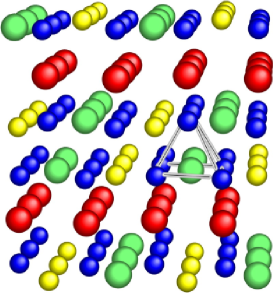
Figure 2: (Color online) Crystal structure of LiCu₂O₂. Green, red, blue and yellow spheres are Cu²⁺, Cu⁺, O and Li ions, respectively.

D. A. Zatsepin et al. Zatsepin have performed the first ab initio calculations of the electronic structure of LiCu₂O₂ in terms of LSDA and LSDA+U approximations. They have concluded that, in the ground state, LiCu₂O₂ is an insulator with ferromagnetic ordering.

A. A. Gippius et al. GippiusMorozova have performed magnetic resonance measurements of LiCu₂O₂ in the paramagnetic and magnetically ordered states. They have also performed full potential LDA calculations. The band structure near Fermi level has been fitted by an extended tight-binding model. Using the resulting hopping parameters, the authors have estimated the values of the exchange interactions $J_{ij}$ within a single band Hubbard model.

Experimental investigations of the magnetic ordering of LiCu₂O₂ by neutron scattering have been performed by T. Masuda et al. Masuda ; Masuda2 The authors have proposed different sets of exchange constants obtained by fitting the calculated spin wave dispersion relation to the experimental curves. None of the sets of parameters is in good agreement with the results of Refs. GippiusMorozova, . One can conclude that, at present, there is no consistent theoretical and experimental description of the magnetic properties of LiCu₂O₂.

In the present paper, the electronic structure calculation of LiCu₂O₂ was performed using the Tight Binding Linear-Muffin-Tin-Orbital Atomic Sphere Approximation (TB-LMTO-ASA) method in terms of the conventional local-density approximation AndersenLDA and crystal structure data from Ref. Berger, . The band structure of LiCu₂O₂ obtained from LDA calculations is presented in Fig.3. There are four bands near the Fermi level which are well separated from others.

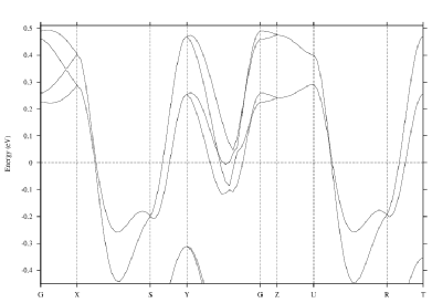
Figure 3: Band structure of LiCu₂O₂ near the Fermi level (0 eV).

These bands are in good agreement with those presented in Ref. GippiusMorozova, .

The partial density of states of LiCu₂O₂ obtained from LDA calculations is presented in Fig.4. Copper 3d states of $x^{2}-y^{2}$ symmetry are strongly hybridized with oxygen 2p states. Therefore it is more natural to use the Wannier function basis rather than atomic orbitals to describe the hybridization processes in LiCu₂O₂. We have used the projection procedure proj which is more accurate than the fitting procedure used in Ref. GippiusMorozova, because the Wannier states in the former method are constructed from all electron DFT orbitals.

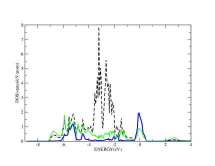
Figure 4: (Color online) Partial density of states obtained from LDA calculations. The blue solid and the dashed lines are the density of copper 3d states of $x^{2}-y^{2}$ symmetry and the total density of 3d states, respectively. The green solid line is the density of oxygen 2p states.

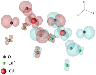
Figure 5: (Color online) Wannier orbitals centered on neighboring copper atoms along y axis.

The resulting Wannier orbitals of LiCu₂O₂, each centered at one Cu site, are shown in Fig.5. One can see that the Wannier orbitals strongly overlap at oxygen and Cu⁺ atoms.

As we mentioned above, one of the possible microscopic mechanisms of exchange interaction is Hubbard-like AF superexchange. This interaction comes from hopping processes. We have calculated the hopping integrals between orbitals of x²-y² symmetry in the Wannier function basis (Table I).

Table 1: Calculated values of hopping parameters $t_{ij}$ between $x^{2}-y^{2}$ orbitals of copper atoms for the one-orbital model and estimated exchange interaction parameters using Eq.(22) (in meV).

	$y$	$2y$	$x$	$\tilde{x}$	$xy$	$\tilde{xy}$	$xyz$
$|t_{ij}|$	54	99	67	5.3	33	28	32
$|t_{ij}|$ (Ref.GippiusMorozova, )	64	109	73	18	25	-	-
$J^{x^{2}-y^{2}}_{ij}$	-24	6.5	3.0	0	0.7	0.5	0.7

The corresponding interaction paths are presented in Fig.6. One can see that for the largest hopping parameters we have good agreement with previous band fitting results.GippiusMorozova However, there are also interaction paths which were not considered before.

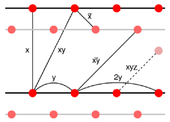
Figure 6: (Color online) The schematic representation of interaction paths between copper atoms in LiCu₂O₂.

For nearest neighbors along the $y$ axis, there is another contribution to the total exchange interaction, namely a FM “direct Coulomb exchange” between Wannier functions. The simplest physical representation of this situation is presented in Fig.7.

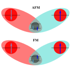
Figure 7: (Color online) Schematic representation of AFM and FM configurations of magnetic moments at Wannier orbitals.

In the case of the AFM configuration, the magnetic moment of the oxygen atom located between two copper atoms vanishes. By contrast, the magnetic moment of the oxygen atom in the FM case is not zero, and the energy gain is $J^{H}_{p}\times\beta^{4}$, where $\beta$ is the contribution of the oxygen atomic orbital to the Wannier orbital (see previous section). In order to calculate the couplings between magnetic moments, we use the following expression, which comes directly from the previous section:

$$J_{ij}=\frac{2t^{2}_{ij}}{\alpha^{4}(U_{d}-V_{dd})+\frac{\beta^{4}J^{H}_{p}N_{ox}}{2}}-\beta^{4}J^{H}_{p}N_{ox},$$ (22)

where $N_{ox}$ is the number of oxygen atoms on which the Wannier orbitals overlap. For simplicity, we neglect the intersite Coulomb interactions. The on-site Coulomb and intraatomic exchange interaction parameters of copper atom are determined from first-principle constrained LDA calculations: $\tilde{U_{d}}$ =10 eV and $\tilde{J}_{d}^{H}$ =1 eV. Therefore the effective Coulomb interaction in Eq.(22) is $U_{d}=\tilde{U_{d}}-\tilde{J}_{d}^{H}$ = 9 eV. The value of the intraatomic exchange interaction of oxygen atom, $J^{H}_{p}$, was estimated in LSDA+U calculations through the shift of oxygen 2p band centers for spin-up, $C_{\uparrow}$ and spin-down, $C_{\downarrow}$: $J^{H}_{p}=(C_{\uparrow}-C_{\downarrow})/M(O)$, where $M(O)$ is the oxygen magnetization. The obtained value of 1.6 eV is in good agreement with previous estimations. Mazin The value of $\alpha^{2}$ is related to the magnetization of copper atoms. Our LSDA+U results (see Table II) show that $\alpha^{2}$=0.58. Since the magnetic moment of the oxygen atom is the result of the magnetization of two copper atoms (see Fig.7), $\beta^{2}$ = M(O)/2 = 0.09. Using Eq.(22) with the parameters defined above, one can calculate the exchange couplings between magnetic moments in LiCu₂O₂. These results are presented in Table I. One can see that the coupling between nearest neighbors along the $y$ axis is strongly ferromagnetic. These model considerations provide a microscopic explanation of the first-principle LSDA+U results presented in the next section.

III.2 LiCu₂O₂: LSDA+U CALCULATION

The analysis of the previous section shows that one should take into account Coulomb on-site correlations and spin polarization of the oxygen atoms. This has been achieved using LSDA+U. The electronic structure of LiCu₂O₂ within LSDA+U is similar to that reported in Ref. Zatsepin, . LiCu₂O₂ is an insulator with an energy gap of 0.7 eV. The values of the calculated magnetic moments (all values in units of $\mu_{B}$) are 0.58 for Cu²⁺ and 0.18 for O.

The next step of the investigation is a first-principle calculation of the isotropic exchange integrals for the Heisenberg model. In order to calculate the couplings between nearest neighbors along the $y$ axis, one should use a method which takes into account the change of magnetization of the oxygen atoms. The most appropriate one is the method Moreira in which the magnetic interaction $J_{ij}$ is estimated through the total energy difference between the ferromagnetic and antiferromagnetic first-principle solutions (obtained, for instance, using the LSDA+U approach).

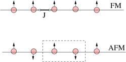
Figure 8: (Color online) Ferromagnetic and antiferromagnetic configurations in an infinite chain with identical nearest neighbor exchange interaction $J$. The dashed line rectangle denotes the unit cell used for the mapping between the Heisenberg model and the first-principle LSDA+U approach.

The Heisenberg Hamiltonian describing the interaction between spins in the unit cell (Fig.8) is given by

$$H=2zJ\vec{S}_{1}\cdot\vec{S}_{2},$$ (23)

where z is number of nearest neighbors. The corresponding total energies of the ferromagnetic and antiferromagnetic configurations of two spins are given by:

$$E_{FM}=2zJS^{2}$$ (24)

and

$$E_{AFM}=-2zJS^{2}.$$ (25)

Therefore the exchange interaction $J$ is expressed in the following form:

$$J=\frac{E_{FM}-E_{AFM}}{4zS^{2}}.$$ (26)

We have performed calculations for the (1 $\times$ 2 $\times$ 1) supercell in ferromagnetic and antiferromagnetic configurations. The results are presented in Table II.

Table 2: Results of LSDA+U calculations for the supercell $1\times 2\times 1$. M(Cu²⁺) and M(O) are magnetic moments of copper and oxygen atoms, respectively. E_tot is the relative total energy (in meV) normalized to 4 (number of copper pairs in unit cell).

	M(Cu2+)	M(O)	Etotal
FM	0.58	0.18	0
AFM	0.58	0	38

One can see that in the case of the ($1\times 2\times 1$) supercell, the magnetization on oxygen atoms for the antiferromagnetic configuration is zero, whereas the compensation of magnetization on oxygen atoms in the ferromagnetic configuration does not take place. Therefore first-principle LSDA+U calculations support the model considerations presented in the previous section. The ferromagnetic configuration has a lower energy than the antiferromagnetic one. Using Eq.(26) with z=2 and S=$\frac{1}{2}$, we get: $J^{y}_{ij}$ = -19.1 meV.

Table 3: Values of exchange interactions J_ij between magnetic moments of LiCu₂O₂ compound (in meV).

	$y$	$2y$	$x$	$\tilde{x}$	$xy$	$\tilde{xy}$	$xyz$
Jij (this work)	-19.1	9.8	3.8	0	1.0	1.0	0.4
Jij (Ref. GippiusMorozova, )	-4	7.2	2.8	0.2	0.4	-	-
Jij (Ref. Masuda2, , Model 1)	-5.95	3.7	0.9	3.2	-	-	-
Jij (Ref. Masuda2, , Model 3)	-7.0	3.75	3.4	0	-	-	-

In order to calculate the other magnetic interactions, we have implemented the Green’s function method. Liechtenstein According to this method, we determine the exchange interaction parameter between copper atoms via the second variation of the total energy with respect to small deviations of the magnetic moments from the collinear magnetic configuration. The exchange interaction parameters J_ij for the Heisenberg model (Eq.(3)) with S=$\frac{1}{2}$ can be written in the following form: Liechtenstein ; Mazurenko

$$J_{ij}=\frac{1}{\pi}\int_{-\infty}^{E_{F}}d\epsilon\,{\rm Im}\sum_{\begin{subarray}{c}m,m^{\prime}\\ m^{\prime\prime},m^{\prime\prime\prime}\end{subarray}}(\Delta^{mm^{\prime}}_{i}\,G_{ij\,\downarrow}^{m^{\prime}m^{\prime\prime}}\,\Delta^{m^{\prime\prime}m^{\prime\prime\prime}}_{j}\,G_{ji\,\uparrow}^{m^{\prime\prime\prime}m})$$

where $m$ ($m^{\prime}$, $m^{\prime\prime}$, $m^{\prime\prime\prime}$) is the magnetic quantum number, the on-site potential $\Delta^{mm^{\prime}}_{i}=H^{mm^{\prime}}_{ii\,\uparrow}-H^{mm^{\prime}}_{ii\,\downarrow}$ and the Green’s function is calculated in the following way

$$G^{mm^{\prime}}_{ij\sigma}(\epsilon)\,=\,\sum_{k,\,n}\frac{c^{mn}_{i\sigma}\,(k)\,c^{m^{\prime}n\,*}_{j\sigma}\,(k)}{\epsilon-E^{n}_{\sigma}}.$$ (27)

Here $c^{mn}_{i\sigma}$ is a component of the nth eigenstate, and E${}_{\sigma}^{n}$ is the corresponding eigenvalue.

Our results are summarized in Table III. One can see that LSDA+U results are in good agreement with those obtained in our model analysis (see previous section) and disagree with previous theoretical estimates. GippiusMorozova This agreement between the model analysis and LSDA+U results is very encouraging, but clearly the ultimate test is to compare them with experiments.

In that respect as well, the present results are a clear improvement with respect to previous estimates. Indeed, in contrast to results of paper Ref. GippiusMorozova, , the ratio between the strongest couplings $J^{2y}_{ij}/J^{y}_{ij}$ = -0.5 is in good agreement with the results of the neutron scattering experiments of Ref. Masuda2, . This ratio is very important since it controls the pitch vector $q$ of the helimagnetic state of LiCu₂O₂. The agreement is not perfect however: Our estimates are about twice larger than the integrals deduced from experiments. Interestingly enough, it is possible, using the simple microscopic model Eq.(22), to identify the source of discrepancy between LSDA+U and experimental results. Indeed, the second term of Eq.(22) is very sensitive to the choice of $\beta^{2}$. For example, $\beta^{2}$=0.08 leads to $J^{y}_{ij}$ = -18.5 meV, which is in excellent agreement with LSDA+U results. For $\alpha^{2}$=0.65 and $\beta^{2}$=0.06, we obtain the following set of model exchange interactions: $J^{y}_{ij}$=-10 meV, $J^{2y}_{ij}$= 5 meV, $J^{x}_{ij}$=2.3 meV, $J^{xy}_{ij}$=0.6 meV, $J^{\tilde{x}y}_{ij}$=0.4 meV and $J^{xyz}_{ij}$=0.5 meV. These model magnetic couplings are in good agreement with the experimental results.

This proves the sensitivity of the results to the precise form of the Wannier functions. Now, it is well known that several sets of localized functions can be used to described a given band, Lechermann and the question of which Wannier functions should be used in the case of the determination of magnetic exchange, a point already raised by Anderson a long time ago, Anderson has not been settled yet. The present results call for further investigation of that issue.

Another possible way however to improve the agreement between theory and experiment could be the following. From the experimental point of view, LiCu₂O₂ has spiral magnetic order in the ground state. Our study was performed for collinear magnetic configurations. Therefore, it would be more natural to calculate the exchange couplings using the magnetic structure observed experimentally. This goes beyond the scope of the present paper however.

IV Discussion

In conclusion, we have presented an analysis of the Hubbard model in the case of nearly 90^∘ metal-oxygen-metal bonds dealing explicitly with Wannier orbitals. This has allowed us to derive an explicit expression of exchange integrals entirely in terms of parameters that can obtained from constrained LDA and LSDA+U. This expression can serve to interpret LSDA+U ab initio estimates of the exchange integrals, and to establish their reliability. The analysis has been applied to the investigation of the magnetic couplings of LiCu₂O₂, allowing us to reach qualitative agreement with experiments, and to gain insight into the nature of exchange in that system. Because of the formation of a strongly hybridized, and energetically isolated combination of $3d_{x^{2}-y^{2}}$ and 2p orbitals, a large moment is transferred to the O ions, and the magnetization of oxygen atoms has been proven to be the main source of ferromagnetism in LiCu₂O₂.

We would like to thank I.V. Solovyev, A.I. Lichtenstein, A.O. Shorikov, J. Dorier and A. Gellé for helpful discussions. The hospitality of the Institute of Theoretical Physics of EPFL is gratefully acknowledged. This work is supported by INTAS Young Scientist Fellowship Program Ref. Nr. 04-83-3230, Netherlands Organization for Scientific Research through NWO 047.016.005, Russian Foundation for Basic Research grant RFFI 04-02-16096, RFFI 06-02-81017 and the grant program of President of Russian Federation Nr. MK-1573.2005.2. The calculations were performed on the computer cluster of “University Center of Parallel Computing” of USTU-UPI. We also acknowledge the financial support of the Swiss National Fund and of MaNEP.

References

- (1) W.Heitler and F. London, Z. Physik 44, 455 (1927).
- (2) W. Heisenberg, Z. Physik 49, 619 (1928).
- (3) P.W. Anderson, Phys. Rev. 115, 2 (1959); Solid State Physics 14, 99 (Academic, New York 1963).
- (4) J. Hubbard, Proc. R. Soc. London, Ser. A 276, 238 (1963)
- (5) G.H. Wannier, Phys. Rev. 52, 191 (1937).
- (6) J.J. Girerd, Y. Journaux and O. Kahn, Chem. Phys. Lett. 82, 534 (1981).
- (7) C. Graaf, I. Moreira, F. Illas, O. Iglesias and A. Labarta, Phys. Rev. B 66, 014448 (2002).
- (8) W. Ku, H. Rosner, W. E. Pickett, and R. T. Scalettar, Phys. Rev. Lett. 89, 167204 (2002).
- (9) A. Huebsch, J. C. Lin, J. Pan, D. L. Cox, Phys. Rev. Lett. 96, 196401 (2006).
- (10) O. Gunnarsson, O.K. Andersen, O. Jepsen, and J. Zaanen, Phys. Rev. B 39, 1708 (1989).
- (11) D.A. Zatsepin et al., Phys. Rev. B 57, 4377 (1998).
- (12) A. A. Gippius et al., Phys. Rev. B 70, 20406 (2004).
- (13) T. Masuda et al., Phys. Rev. Lett. 92, 177201 (2004).
- (14) T. Masuda et al., Phys. Rev. B 72, 014405 (2005).
- (15) O.K. Andersen, Z. Pawlowska and O. Jepsen, Phys. Rev. B 34, 5253 (1986).
- (16) R. Berger, J. Alloys Compd. 184, 315 (1992).
- (17) V.I. Anisimov et al., Phys. Rev. B 71, 125119 (2005).
- (18) I.I Mazin and D.J. Singh, Phys. Rev. B 56, 2556 (1997).
- (19) Iberio de P.R. Moreira and F. Illas, Phys. Rev. B 55, 4129 (1997).
- (20) A.I. Lichtenstein, M.I. Katsnelson, V.P. Antropov, and V.A. Gubanov, J. Magn. Magn. Mater. 67, 65 (1987).
- (21) V.V. Mazurenko and V.I. Anisimov, Phys. Rev. B 71, 184434 (2005).
- (22) See e.g. F. Lechermann, A. Georges, A. Poteryaev, S. Biermann, M. Posternak, A. Yamasaki, and O. K. Andersen, Phys. Rev. B 74, 125120 (2006), and references therein.