Properties of low density quantum fluids within nanopores

Abstract

The behavior of quantum fluids (⁴He and H₂) within nanopores is explored in various regimes, using several different methods. A focus is the evolution of each fluid’s behavior as pore radius $R$ is increased. Results are derived with the path integral Monte Carlo method for the finite temperature ($T$) behavior of quasi-one-dimensional (1D) liquid ⁴He and liquid H₂, within pores of varying $R$. Results are also obtained, using a density functional method, for the $T=0$ behavior of ⁴He in pores of variable $R$.

I Introduction

The behavior of quantum fluids (e.g. helium or hydrogen) in reduced dimensionality is one of the most interesting topics in low temperature physics.ref1 Among the systems of particular interest are monolayer films (which are effectively two-dimensional, or 2D) and fluids within narrow pores (1D) or droplets (0D).ref2 ; ref3 ; ref4 ; ref5 ; ref6 ; ref7 Properties associated with phase transitions (e.g. critical exponents) are particularly sensitive to the dimensionality, as exemplified by the Kosterlitz-Thouless theory of the 2D superfluid transition in He films.ref8 Confined ideal gases are particularly amenable to theoretical study, because one need solve just the single particle Schrödinger equation in the given environment, rather than the fully interacting many-body problem.ref7 Such an idealized model can provide qualitatively, and sometimes quantitatively, reliable predictions of the effects of confinement on the fluid. Furthermore, these calculations can be supplemented, in some cases, by virial expansions in order to assess the role of interactions, presuming their effects to be weak.ref9 ; ref10 In contrast, dense quantum fluids require the use of the path integral Monte Carlo (PIMC) or diffusion Monte Carlo methods, which are computationally demanding approaches. Nevertheless, these techniques has been applied in recent years to many problems of reduced dimensionality.ref11 ; ref12

Considerable progress in understanding $D<3$ behavior has also been achieved on the experimental front. Although the evolution of superfluidity in thin films was first observed in heat capacity experiments nearly 70 years ago, that subject remains incompletely understood.ref13 The problem of quantum droplets has received particular attention in recent years, stimulated especially by the search for superfluid hydrogen.ref6 ; ref14 ; ref15 The discovery of carbon nanotubes and interest in other quasi-1D porous media have led to many investigations of 1D quantum fluids.ref5 ; ref16 ; ref17

This paper addresses a set of problems involving helium and hydrogen within small radius ($R$) cylindrical pores, such as carbon nanotubes. For $R\sim 0$, one encounters the strictly 1D limit of a quantum fluid. While there has been considerable exploration of the zero temperature ($T$) behavior of such systems, relatively few studies of finite $T$ behavior of the interacting system have been carried out.ref12 ; ref17 ; ref18 ; ref19 ; ref20 ; ref21 ; ref34 In a recent study, we explored such behavior for 1D ⁴He. It was demonstrated that a 1D phonon model, analogous to the Landau hydrodynamic theory of liquid ⁴He, does describe the behavior at low $T$ of 1D ⁴He at moderate to high density (compared to the equilibrium density $\rho=0.036$/Å).ref22 Section II of the present paper presents a finite range density functional study of the behavior of ⁴He, at temperature $T=0$, as $R$ is varied. The results exhibit the evolution of the system from an essentially 1D “axial phase” to a “cylindrical shell” phase, localized near the pore walls.ref16 ; ref23 Section III shows how the behavior of H₂ at finite $T$, but low density, varies with pore radius $R$. Section IV summarizes our results.

II Liquid ⁴He in a nanopore at zero temperature

As shown in previous work, finite-range density functional (FRDF) calculations permit the calculation of the equation of state (EOS) of helium atoms in various environments (see, e.g., Barranco et al.ref15 and references therein). In this section, we investigate the condensation of helium in a cylindrical pore of radius $R$ and length $L$, with the same density functional employed in Refs. ref24, ; ref25, ; ref26, , with detailed description and parameters found in Ref. ref27, . The calculation is based on the energy density $\mathcal{E}[\rho(r)]$, where $\rho(r)$ is the particle density, normalized to the total number of helium atoms $N$ so that, in the pore geometry, the linear density (over $2\pi$), $n=N/(2\pi L)$, is

$$n=\int dr\,r\rho(r)\,.$$ (1)

The total energy $e=E/(2\pi L)$ per unit length (over $2\pi$) is then

$$e=\int dr\,r\mathcal{E}[\rho(r)]\,.$$ (2)

The Euler-Lagrange equation for the density is obtained by functional differentiation of this energy with respect to $\rho(r)$, at fixed total number of particles, and takes the form

$$\Bigl{[}-\frac{\hbar^{2}}{2m}\Bigl{(}\frac{d^{2}}{dr^{2}}+\frac{1}{r}\frac{d}{dr}\Bigr{)}+U(\rho)+V(r;R)\Bigr{]}\sqrt{\rho(r)}=\mu\sqrt{\rho(r)}\,,$$ (3)

with $\mu$ the chemical potential, $U(\rho)\equiv\delta E/\delta\rho(r)$ the density-dependent mean field and $V(r;R)$ the adsorption potential provided by the cylindrical sheet. This function was derived by considering that a He atom at radial distance $r$ from the axis of the cylinder interacts pairwise with continuum sheet of atoms, of uniform areal density $\theta$, via a Lennard-Jones (LJ) potential of well-depth $\epsilon$ and hard core diameter $\sigma$. The result is expressed in terms of elliptic integrals defined in Ref. ref23, :

$$V(r;R)=3\pi\epsilon\sigma^{2}\theta\Bigl{[}\frac{21}{32}\Bigl{(}\frac{\sigma}{R}\Bigr{)}^{10}M_{11}(r/R)-\Bigl{(}\frac{\sigma}{R}\Bigr{)}^{4}M_{5}(r/R)\Bigr{]}\,.$$ (4)

Here $M_{2n+1}$ is an elliptic integral over angle $\phi$.

Prior to determining the EOS of liquid He in pores, we consider the binding of a single He atom to an alkali metal cylindrical sheet. In particular, Cs substrates of diverse shapes are excellent candidates to investigate nontrivial aspects of the physics of wetting. While the He-Cs potential is too weakly attractive to adsorb He on a flat Cs surface (below saturation chemical potential $\mu_{0}$), there are two reasons why He does adsorb within a pore. One is that the surface tension cost of pore-filling is smaller than that on a planar surface (by a factor of tworef28 ). The other is that the potential can be substantially enhanced within a concave environment, either a pore or a wedge of intermediate openings.ref27

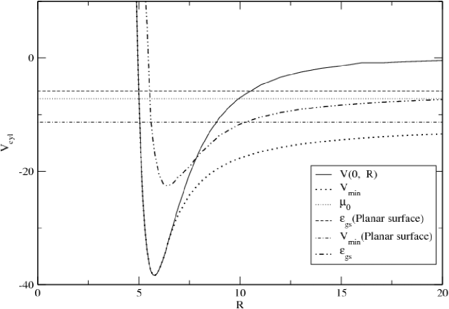
Figure 1: Cylindrical potential $V(0,R)$ on the axis, potential $V_{\mathrm{min}}$ at the absolute minimum, and ground state energy $\varepsilon_{gs}$ of a ⁴He atom. For reference, the bulk chemical potential $\mu_{0}$, the minimum potential of a planar Cs sheet $V_{\mathrm{min}}$ (planar surface) and corresponding energy $\varepsilon_{gs}$ (planar surface) are also displayed.

Illustrative results are shown in Figs. 1 and 2. In Fig. 1 we plot, as functions of cylinder radius $R$, the potential $V(0,R)$ on the cylinder axis, the potential $V_{\mathrm{min}}$ at the absolute minimum of $V(r,R)$, and the ground state (gs) energy $\varepsilon_{gs}$ of one atom obtained by solving the single-particle (sp) Schrödinger equation in the cylindrically symmetric potential. The ⁴He bulk chemical potential $\mu_{0}=-7.15$ K is displayed as a reference, as well as the minimum potential $V_{\mathrm{min}\infty}=-11.3$ K of a planar Cs sheet and the corresponding gs energy $\varepsilon_{gs\infty}=-5.83$ K. We note that the absolute minimum departs from the axis at a radius of about 6.8 Å. On the other hand, the sp energy drops below the potential on the axis around $R=7.5$ Å, corresponding to an approximate threshold radius for the off-axis displacement of the maximum probability density $\lvert\psi(r)\rvert^{2}$. This behavior is illustrated in Fig. 2, where the upper panel displays the potentials due to Cs sheets of varying radius $R$, as functions of the radial distance $r$, and the lower panel shows the probability density of the He atom. The parameters of the He-Cs interaction are $\epsilon=2.795$ K, $\sigma=5.31$ Å, and $\theta=0.38$/Ų. The large value of $\sigma$ reflects the extent of the hard-core repulsion for this interaction, which is responsible for the weak van der Waals attraction, i.e., the small value of $\epsilon$.

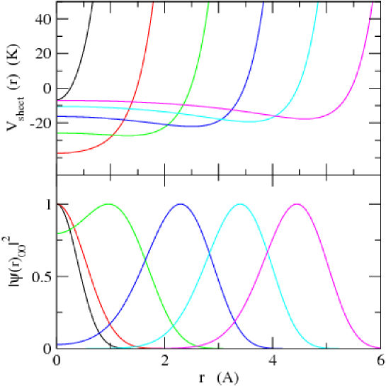
Figure 2: Upper panel: potentials of a He atom inside Cs cylinders of radius for $R$ values between 5 and 10 Å, from left to right in steps of 1 Å. Lower panel: corresponding probability density of one atom in its ground state. The 3D probability distributions have been normalized to unit maximum value.

For the smallest radii displayed, 5 and 6 Å, the probability density for this “axial phase” is seen to be concentrated on the axis, while for the largest radii, 9 and 10 Å, the particle is localized (with spread $\sim 1.2$ Å) about 5.6 Å from the wall; for this “cylindrical shell” phase, the latter distance asymptotes to $\sigma=5.31$ Å for the hypothetical limiting case $R=\infty$. In the intermediate $R$ regime, there remains a non-negligible probability density at $r=0$, seen to be quite sizable for $R=7$ Å. Note that the atom is unbound (relative to vacuum) in a 5 Å tube; in fact, according to Fig. 1, the gs energy is negative for radii larger than 5.2 Å. Thus, a noninteracting Bose gas will be bound within such pores in a quasi-1D axial phase, a filled pore regime and a quasi-2D shell phase, as $R$ increases. For even larger $R$, the usual layering structure of helium in a cavity occurs.ref16 ; ref26

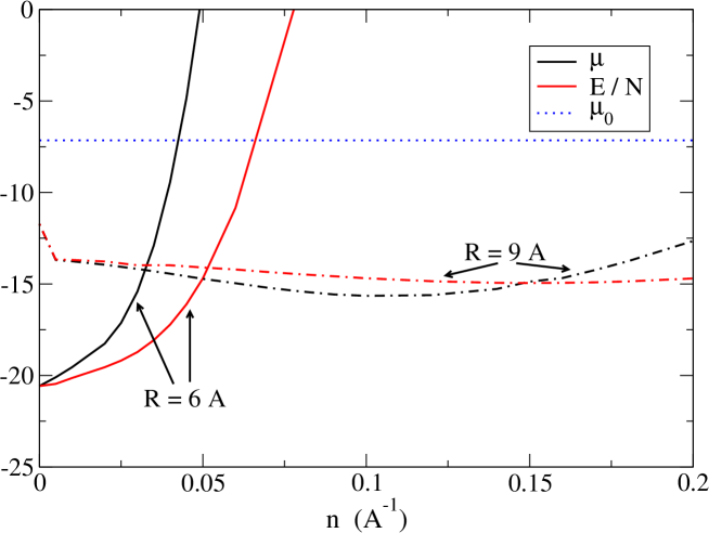
Figure 3: Chemical potential (black) and energy per particle (red) for liquid He in Cs pores of radii $R=6$ and 9 Å, as functions of linear density. The bulk chemical potential $\mu_{0}$ is shown as a dotted line.

Next, we explore the many-body behavior by solving Eq. 3 to obtain the chemical potential $\mu$, the total energy, and the density profiles $\rho(r)$, as functions of the linear density $n$. Significant results are presented in Fig. 3, which shows $\mu$ and the energy per particle for two selected pore radii, namely $R=6$ and 9 Å, in full and dashed lines, respectively. For the narrower pore, a stable quasi-one-dimensional (Q1D) system with negative grand potential per unit length, $\omega=e-\mu$, is found for any linear density below $0.042$ Å^-1, above which the system becomes unstable. For a sufficiently wide pore, the particle distribution has moved towards the cylinder wall and the EOS displays the typical 2D prewetting jump at $n_{pw}=0.15$ Å^-1, at which point the energy per particle becomes identical to the chemical potential, resulting in condensation of a stable film at this or higher linear densities. This behavior can be assessed by examining density profiles for various values of $R$ at a given linear density, as displayed in Fig. 4 for $n=0.05$ Å^-1. In this figure, the upper panel shows both the confining potential and the total one-body field $U[\rho(r)]+V(r;R)$ experienced by particles in the fluid. The resulting particle densities are plotted in the lower panel as functions of distance $r$.

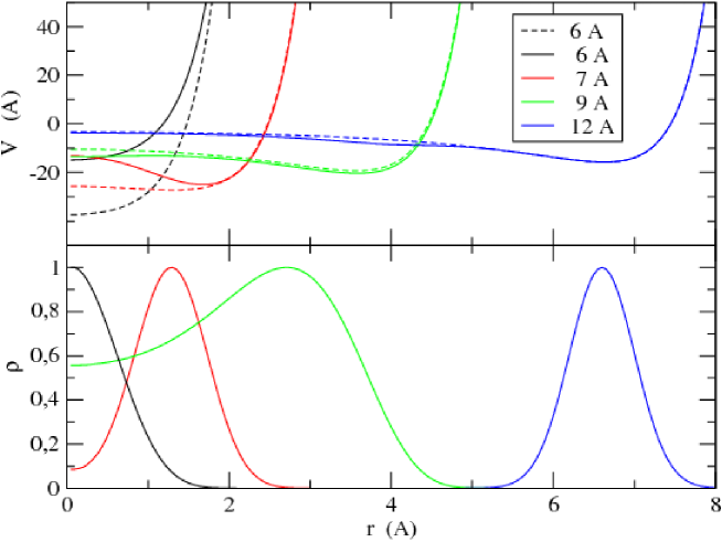
Figure 4: Upper panel: total mean-field potential in Eq. 3 (full lines) and potentials $V(r,R)$ from the Cs cylinder for radii $R=6$, 7, 9 and 12 Å (from left to right). Lower panel: corresponding particle densities (normalized to unit maximum) at a linear density $n=0.05/$Å.

At first sight, in Fig. 4 we note the presence of the three distinct regimes of density behavior, as encountered in the sp pattern displayed in Fig. 2. In addition, this plot provides evidence of the effect of cohesion among the He atoms and its competition with the weak adhesion to the confining walls. The difference between full and dashed lines is the total interaction energy (per particle) of the interacting fluid, as shown in various prior studies.ref24 ; ref25 ; ref26 ; ref27 This total consists of a screened LJ interaction plus two density-dependent correlation terms, one attractive, the other repulsive, representing the effects of the many-body environment on the one-body field. For the two smallest radii, the overall outcome, as seen in the upper panel of Fig. 4, is a visible reduction in potential energy and a distortion of the potential well that causes an earlier departure of the minimum off-axis, as compared with the sp picture in Fig. 2. The situation is reversed for the largest radii. For $R=9$ Å, the potential energy gain of about 2 K near the cylinder axis is sufficient to sustain a non-negligible amount of fluid in that region. As a consequence, pores of radii between somewhat less than 7 Å and more than 9 Å result in a particle density spread out from axis to wall, and the appearance of the purely axial regime shifts towards larger radii. For radii near 12 Å and above, instead, the correlation effects in the helium fluid are negligible and the system behaves essentially as a confined gas.

III H₂ in a nanopore at finite $T$

We consider in this section the adsorption of H₂ (which, after ⁴He, is the textbook quantum fluid) molecules inside a cylindrical pore within a bulk solid. As in the preceding section, a low density gas of molecules within a large pore will typically adsorb first onto the inner surface of the pore, creating a 2D cylindrical shell phase at low densities; at higher densities, central regions of the pore will fill with a 3D bulk adsorbate.ref16 Very narrow pores, however, will constrain the adsorbate to lie near the pore axis, forming a quasi-1D (“axial”) phase. This variation of behavior provides the opportunity to control the effective dimensionality of the adsorbate by adjusting the size of the pore into which it adsorbs. For concreteness, we chose to study pores in MgO glass, a much more strongly adsorbing substrate than the Cs discussed in the previous section; the well-depth (48 meV) of an H₂ molecule on planar MgO is about 15 times higher than that on Cs. ref29 ; ref30 MgO nanopores can be fabricated as small as 3 nm in diameter.ref43 The H₂-MgO potential was taken to be derived from Lennard-Jones 12-6 pair interactions, integrated over the bulk MgO solid; these gas-surface interaction parameters are given by $\sigma=2.014$ Å, $\epsilon=45.91$ K. The H₂-H₂ interaction potential was taken to be of the Silvera-Goldman form.ref31 The molecule is treated as a spherically symmetric point particle, neglecting internal degrees of freedom.

III.1 Structure: path integral Monte Carlo simulations

This quantum statistical system can be simulated by the path integral Monte Carlo (PIMC) method.ref11 ; ref33 The simulations were performed for various pore radii $R$ at fixed temperature $T=0.5$ K (or 1 K) and particle number $N=28$; the mean 3D density $\bar{\rho}=N/V$ changed as the pore volume was varied. The value $N=28$ was chosen to approximate the equilibrium linear density of a 1D system of fixed length (of the periodic unit cell) $L=125$ Å.ref34 ; ref35 The value of $L$ was chosen large enough to ensure that finite size effects were minimal, as confirmed by simulation tests.ref36

The distribution of H₂ molecules calculated by PIMC simulation is given in Fig. 5 for several pore sizes. The axial-to-shell transition is more apparent in Figure 6, which shows the H₂ radial density distribution, along with the corresponding H₂-pore potential energy curves. Classically, the molecules will concentrate on axis when the potential minimum is at $r=0$, and will move off axis when the minimum is found at some $r>0$, if intermolecular interactions are neglected (the low density limit). The PIMC simulations at low densities indicate that the adsorbate moves off axis between pore radii of $R=2.5$ and 2.75 Å; by comparison, the classical potential minimum moves off axis at slightly smaller pore size, $R=2.35$ Å. In other words, the molecules tend to concentrate near the axis more when treated as quantum particles than when treated classically. The comparison between quantum and classical behavior in this system is discussed more fully in the following section.

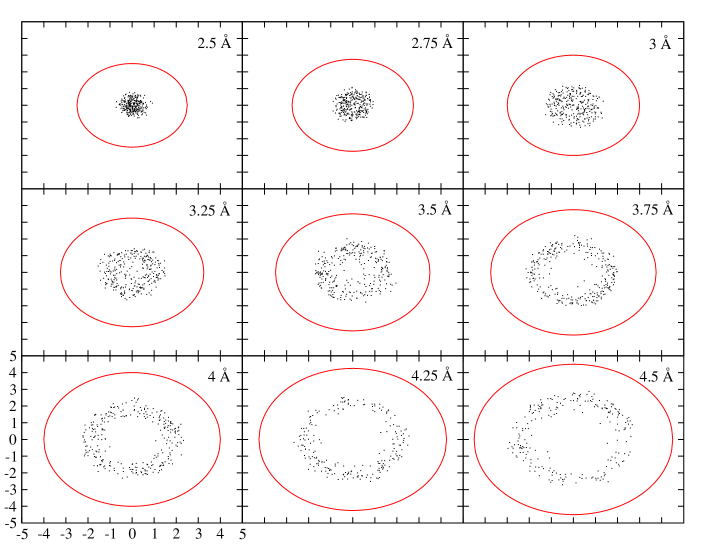
Figure 5: H₂ density distribution [at $T=0.5$ K, $\bar{\rho}=(2.55\times 10^{-3}$ Å)$/R^{2}$], viewed in transverse section, for pore radii $R=2.5$–$4.5$ Å, as indicated. Depicted are several hundred superimposed Monte Carlo samples of particle positions (dots) for a system of $N=28$ particles, along with the inner surface of the pore (circles). (The circles are distorted into ellipses due to the aspect ratio of the figure.) The H₂ evolves from a 1D (axial) to a 2D (cylindrical shell) phase as $R$ increases.

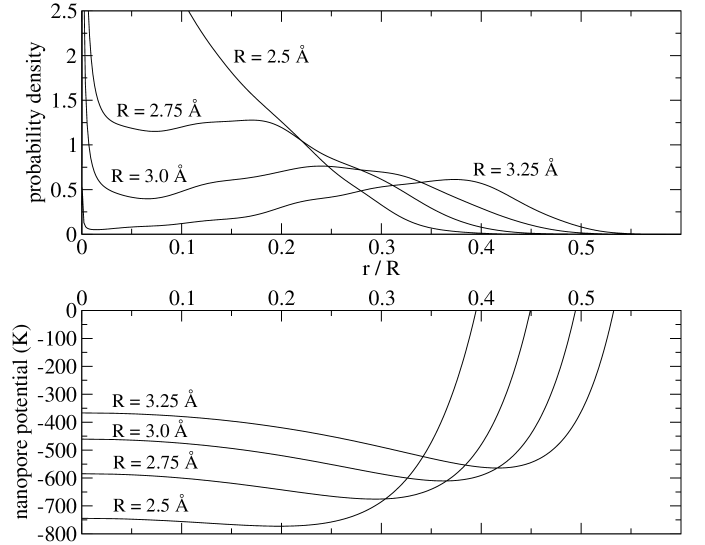
Figure 6: H₂ probability density [at $T=0.5$ K, $\bar{\rho}=(2.55\times 10^{-3}$ Å)/$R^{2}$] and MgO pore potential, for pore radii $R=2.5$, 2.75, 3.0 and 3.25 Å, as functions of dimensionless radius $r/R$. (Radial densities near $r=0$ are exaggerated due to finite size effects after normalizing the radial distribution by $1/(2\pi r)$ to obtain the probability density.)

A closer examination of samples drawn from Monte Carlo simulation, Fig. 7, reveals the presence of bound H₂-H₂ pairs, or “dimers”, as well as possible bound triplets, or “trimers”. Such clustering is expected below a temperature set by the H₂-H₂ binding energy. This visual evidence is corroborated quantitatively by the pair correlation function derived from PIMC simulation, Fig. 8, which shows an enhanced probability for H₂ molecules to be separated by $r=4.8$ Å. By comparison, the classical equilibrium separation of a pair of H₂ molecules is $r=3.4$ Å; the separation of quantum H₂ is greater due to zero-point fluctuations, which reduce the binding energy to about 3 K, roughly one-tenth of the well-depth of the pair potential.ref31 ; ref37

Figure 7: H₂ spatial density distribution (at $T=1$ K, average density $\bar{\rho}=1.46\times 10^{-3}$/ų), for $N=28$ particles in a pore of radius 7 Å. Depicted are two individual Monte Carlo samples of particle positions. (The scale of the vertical, longitudinal axis is compressed relative to that of the transverse axes.) Note the presence of dimers (H₂-H₂ pairs) in both plots, as well as possible trimers.

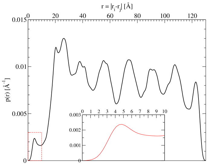
Figure 8: H₂ pair correlation function (at $T=1$ K, $\bar{\rho}=1.46\times 10^{-3}$/ų), for $N=28$ particles in a pore of radius 7 Å. Inset: An expanded view of the pair correlation function, near the $r=4.8$ Å peak, that indicates the presence of dimerization.

In a crude analysis of Fig. 7, we estimate that at $T=1$ K approximately equal numbers of H₂ molecules participate in monomers (unpaired H₂) as dimers, i.e. a dimer/monomer ratio of 0.5. This quantity can be roughly estimated by assuming that the monomer$\Leftrightarrow$dimer process is in detailed balance, implying that their respective chemical potentials, $\mu_{1}$ and $\mu_{2}$, satisfy $\mu_{2}=2\mu_{1}$. Assuming the H₂ to be an ideal gas of $N$ molecules, the chemical potentials are related to the individual populations ($N_{i}$) by

$$\begin{split}\mu_{1}&=k_{B}T\ln\Bigl{(}\frac{N_{1}\lambda_{1}^{D}}{eV}\Bigr{)}\,,\\ \mu_{2}&=k_{B}T\ln\Bigl{(}\frac{N_{2}\lambda_{2}^{D}}{eV}\Bigr{)}-\epsilon\,,\end{split}$$ (5)

where $\lambda\equiv\sqrt{2\pi\hbar^{2}/(mk_{B}T)}$ is the thermal wavelength and $\epsilon$ is the binding energy per dimer. These relations, under the constraint $N=N_{1}+2N_{2}$, give a dimer/monomer ratio

$$\frac{N_{2}}{N_{1}}=\frac{1+4x-\sqrt{1+8x}}{2(\sqrt{1+8x}-1)}\,,\qquad x\equiv 2^{D/2}\Bigl{(}\frac{\bar{n}}{n_{Q}}\Bigr{)}e^{\epsilon/(k_{B}T)}\,.$$ (6)

Here $\bar{n}=N/V$ is the mean 3D number density and $n_{Q}=1/\lambda^{D}$ is the quantum concentration. For $N=28$ H₂ molecules at $T=1$ K in a 3D volume $V=\pi R^{2}L$, where $R=7$ Å and $L=125$ Å, assuming their binding energy is $\epsilon=3$ K, Eq. 6 predicts a dimer-monomer ratio of 8.5. This estimate exceeds the ratio observed in PIMC simulation by an order of magnitude. However, the preceding back-of-the-envelope calculation is expected to have limited accuracy since it ignores the quasi-2D geometry of adsorption, the presence of internal rotational-vibrational excitational modes of the dimer and the possibility of trimer, or larger, clusters of bound molecules.

III.2 Structure: semiclassical approximation

As mentioned above, the axial and shell phases can be distinguished in the classical, noninteracting case by the location of the potential minimum ($r=0$ or $r>0$) for a given pore radius $R$. Quantum mechanically, one must resort to either solving the Schrödinger equation and finding the peak probability from the radial wavefunction (for the noninteracting case) or by carrying out a full path integral Monte Carlo simulation (in the general interacting case).

Besides their use in Monte Carlo simulations, the path integral method also yields a semiclassical approximation to the density that is almost as simple as inspection of the classical potential. A variational approximation, originally due to Feynman, reduces the quantum statistical path integral to the ordinary Boltzmann integral of classical statistical mechanics, with the classical potential V replaced by a semiclassical effective potential $V_{\mathrm{eff}}$ containing first-order quantum corrections to V.ref38 This potential is expressed as a weighted average of the real potential over a distance comparable to the de Broglie thermal wavelength. Thus, in this approximation, the axial phase of quantum H₂ occurs when the minimum of the effective potential lies at $r=0$. Feynman’s variational approximation yields a formula for $V_{\mathrm{eff}}$ as a functional of the classical potential in the case of a noninteracting quantum gas,

$$V_{\mathrm{eff}}(\mathbf{r})=(2\pi\Lambda^{2})^{-3/2}\int d^{3}\mathbf{r}^{\prime}\,V(\mathbf{r}^{\prime})\exp{\Bigl{[}-\frac{1}{2}(\lvert\mathbf{r}-\mathbf{r}^{\prime}\rvert/\Lambda)^{2}\Bigr{]}},\qquad\Lambda\equiv\hbar/\sqrt{12mk_{B}T}\,.$$ (7)

Here $m$ is the mass of a particle, in this case an H₂ molecule. This has a high-temperature expansion

$$V_{\mathrm{eff}}=V+\frac{1}{2}\Lambda^{2}\nabla^{2}V+O(\Lambda^{4})\,.$$ (8)

The effective potential in Eq. 7 is the convolution of the classical potential with a Gaussian of width $\Lambda$, and may be interpreted as a “quantum smeared” version of the classical potential. In the high temperature (small $\Lambda$) limit, the smearing vanishes, and the effective potential reproduces the classical result. In the case of cylindrical symmetry, these equations become

$$V_{\mathrm{eff}}(r)=\Lambda^{-2}\int_{0}^{\infty}dr^{\prime}\,V(r^{\prime})\,r^{\prime}\,I_{0}\Bigl{(}\frac{rr^{\prime}}{\Lambda^{2}}\Bigr{)}\exp{\Bigl{[}-\frac{1}{2}(r^{2}+{r^{\prime}}^{2})/\Lambda^{2}\Bigr{]}}\,,$$ (9)

and

$$V_{\mathrm{eff}}=V+\frac{1}{2}\Lambda^{2}(V^{\prime\prime}+V^{\prime}/r)+O(\Lambda^{4})\,.$$ (10)

Effective potentials for various $R$ and $T$ values are displayed in Figure 9. As expected, $V_{\mathrm{eff}}$ approaches $V$ as $T$ increases. The main qualitative results concern the location of the effective potential minimum. This energy is greater than that of the classical potential minimum, due to the zero point energy. It is also located closer to the axis, because the repulsive hard wall of the potential at $r=R$ damps the wavefunctions of quantum particles in the repulsive region.

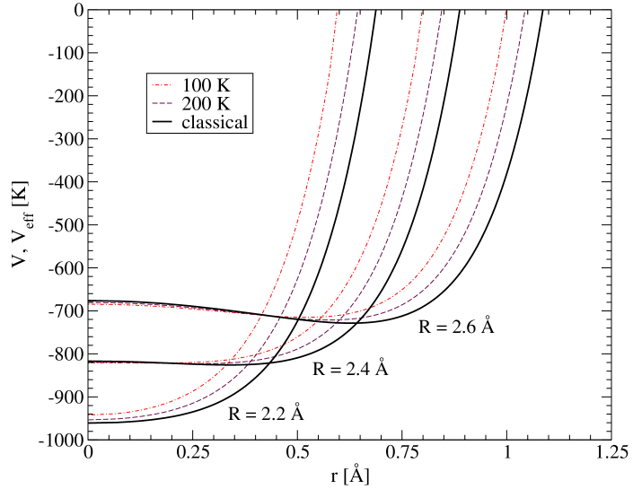
Figure 9: H₂-MgO pore radial effective potentials at $T=100$ and 200 K, compared to the corresponding classical potentials, at pore radii $R=2.2$, 2.4, and 2.6 Å. Note that the quantum behavior described by the effective potential approaches classical behavior in the high temperature limit.

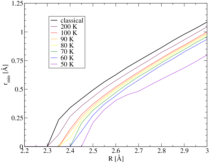
Figure 10: Minimum of the H₂-MgO pore radial effective potential, $r_{\mathrm{min}}$, as a function of pore radius $R$, for various temperatures (increasing from lower right to upper left), compared to the minimum of the classical potential (upper leftmost curve). The axial/shell transition occurs at the radius $R$ for which $r_{\mathrm{min}}$ becomes nonzero. This transition point for the quantum gas is the same as the classical transition of $R=2.3$ Å when $T=200$ K, and increases to 2.45 Å as the temperature of the quantum gas decreases to $T=50$ K. (The resolution of the plot and therefore the precision of the estimated transition point is calculated to within 0.05 Å.)

Qualitatively, then, these semiclassical considerations imply that a quantum gas has a greater tendency to be confined near the axis than does a classical gas, agreeing with the preceding results obtained by PIMC simulation. Quantitatively, the semiclassical approximation breaks down at temperatures above the $T=0.5$ K studied by PIMC, but one may use it for qualitative purposes. For example, the location of the effective potential minimum at higher temperatures ($T>50$ K) is given in Figure 10. Note that the classical potential minimum moves off axis near $R=2.30$–2.35 Å, while the effective potential minimum moves off axis near 2.35 Å at 100 K and near 2.45 Å at 50 K. By extrapolation of these semiclassical predictions, it is plausible that the low $T$ axial-shell transition occurs between 2.50 and 2.75 Å, as found in the preceding section by PIMC simulation at $T=0.5$ K.

III.3 Heat capacity

In accordance with the structural results of the preceding sections, the heat capacity $C\equiv(\partial E/\partial T)_{N,V}$ of the H₂ is expected to exhibit 1D behavior for small $R$, and 2D behavior for larger $R$ pores. In the ideal gas approximation, for small $R$, the single longitudinal degree of freedom should give a dimensionless specific heat, or heat capacity per particle (in $k_{B}=1$ units) of 1/2, in accordance with the equipartition theorem. An additional azimuthal degree of freedom is available in the cylindrical shell phase of larger $R$, increasing $C/(Nk_{B})$ to 1, given enough thermal energy to overcome the azimuthal excitation energy gap. At very high $T$, the large radial excitation energy gap will be exceeded, allowing an additional degree of freedom, raising the specific heat to 3/2.

In the noninteracting case, the heat capacity can be calculated by direct differentiation of the average energy, upon obtaining the energy spectrum from numerical solution of the Schrödinger equation. In the grand canonical ensemble, the average particle number and energy of a Bose gas are given by summing the Bose-Einstein distribution of states over all possible energies (weighted by the density of states, or relative prevalence of each energy); this includes an integration over the continuum of longitudinal energies as well as a summation over the discrete spectrum of radial/azimuthal transverse energies $\varepsilon_{n,\nu}$. These quantities are then given by

$$N(\beta,\mu) =\sum N_{\varepsilon}=\sum_{n,\nu=0}g_{\nu}\int dE\,\frac{g(E)}{z^{-1}\exp[\beta(E+\varepsilon_{n,\nu})]-1}\,,$$ (11)

$$E(\beta,\mu) =\sum E_{\varepsilon}=\sum_{n,\nu=0}g_{\nu}\int dE\,\frac{g(E)}{z^{-1}\exp[\beta(E+\varepsilon_{n,\nu})]-1}\,,$$ (12)

where $z$ is the fugacity [$\exp(\beta E)$], $\mu$ is the chemical potential, $\beta=1/(k_{B}T)$ is the inverse temperature, $g(E)=(L/\lambda)[\beta/(\pi E)]^{1/2}$ is the density of states for a 1D (longitudinal) gas, and the degeneracy $g_{\nu}$ is 1 for $\nu=0$ (no angular momentum) and 2 for $\nu>0$ [corresponding to the $\pm$(counter-)clockwise azimuthal states].

Fixing the particle number $N$, the first equation is used to solve $\mu$ in terms of particle number, $\mu(N)$, which is substituted into the second equation to determine the average energy $E(T,N)$. The specific heat $c=C/N$, or heat capacity per particle, is obtained by a finite difference approximation to the derivative $[\partial(E/N)/\partial_{T}]_{N,V}$.

The resulting dimensionless specific heat as a function of $R$, at $T=1$ and 5 K, is depicted in Figure 11 (Also shown are predictions for a quasi-1D approximation, in which only the azimuthal ground and first excited states are considered, not discussed further here.) The evolution of the specific heat from 1/2 for small $R$ to 1 for large $R$ is readily apparent. The small $R$ specific heat is less than the classical prediction of $1/2$ because the temperatures are low enough that the quantum system has not reached the classical limit; it is closer to 1/2 for the more classical $T=5$ K case than for the lower temperature, $T=1$ K, case.

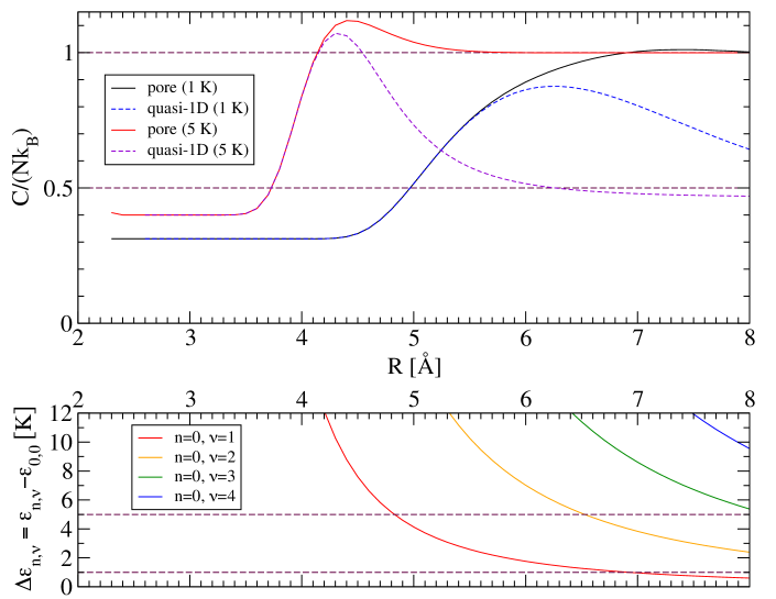
Figure 11: Above: Specific heat of noninteracting H₂ gas in a MgO pore as a function of pore radius $R$, at fixed mean linear density $N/L=0.224$ Å^-1 [mean 3D density $\bar{\rho}=N/L/(\pi R^{2})$], for $T=1$ and 5 K (right and left solid curves). Contrasted are the predictions of the quasi-1D model with an energy gap $\varepsilon\equiv\varepsilon_{0,1}-\varepsilon_{0,0}$ determined by the ground state and first azimuthal state (dashed curves). (The quantum numbers $n,\nu$ of $\varepsilon_{n,\nu}$ denote radial and azimuthal excitations, respectively.) The horizontal dashed lines are the classical 1D and 2D limits of $\frac{1}{2}$ and 1, respectively. Below: The energy gap between the ground state ($\varepsilon_{0,0}$) and the first four azimuthal excitations of the ground radial state ($\varepsilon_{0,\{1\ldots 4\}}$, increasing from left to right). The horizontal dashed lines correspond to energy gaps of 1 and 5 K.

The higher $T$ case approaches the 2D limit more quickly, since more thermal energy is available to excite the higher azimuthal modes that contribute the additional degree of freedom necessary for 2D motion. Structurally, in the PIMC simulation at $T=0.5$ K, the H₂ changed from an axial to a shell-like configuration for $R<3$ Å. The heat capacity, on the other hand, indicates a transition from 1D to 2D behavior at larger $R\sim 6$ Å at $T=1$ K. Thus, the H₂ may behave thermodynamically as a 1D gas even when it is structurally arranged as a 2D film. At pore sizes of $R=4$ Å, the pore is large enough for a shell configuration to be energetically favorable, yet the azimuthal energy gap, which shrinks with increasing $R$, is not yet large enough to permit appreciable rotational motion leading to an enhanced heat capacity. (The energy gaps of the first few azimuthal excited states are also depicted in Fig. 11.)

IV Summary

Results have been obtained for the $T=0$ properties of liquid ⁴He and finite $T$ properties of liquid H₂. In both cases, the behavior is seen to exhibit dimensional crossover as a function of $R$, as shown in the density profiles and thermodynamic properties (energies, chemical potentials and specific heat). A wide variety of other properties, including detailed dependences on $N$ and $T$, are amenable to further theoretical investigation. While we hope to undertake some of these investigations in the future, they require a substantial increase in computational resources and time. Nevertheless, these are justified by recent experimental studies of quantum fluids in and near carbon nanotubes and other porous media.ref39 ; ref40 ; ref41 ; ref42

- (1) H. Taub, G. Torzo, H. J. Lauter, and S. F. Fain, Jr., eds., Phase Transitions in Surface Films 2 (Plenum, New York, 1991).
- (2) O. E. Vilches, Ann. Rev. Phys. Chem. 31, 463 (1980).
- (3) L. W. Bruch, M. W. Cole, and E. Zaremba, Physical Adsorption: Forces and Phenomena (Oxford University Press, New York, 1997).
- (4) E. Krotscheck and J. Navarro, eds., Microscopic Approaches to Quantum Liquids in Confined Geometries (World Scientific, Singapore, 2002).
- (5) M. M. Calbi, M. W. Cole, S. M. Gatica, M. J. Bojan, and G. Stan, Rev. Mod. Phys. 73, 857 (2001).
- (6) “Helium nanodroplets: a novel medium for chemistry and physics”. J. Chem. Phys. 115(22), 10065–10565 (2001).
- (7) J. G. Dash, Rev. Mod. Phys. 71, 1737 (1999); D. E. Shai, M. W. Cole, and P. E. Lammert, “Adsorption of quantum gases on curved surfaces”, to appear in J. Low Temp. Phys.
- (8) J. M. Kosterlitz and D. J. Thouless, in Progress in Low Temperature Physics, Vol. 7B, edited by D. F. Brewer (North Holland, New York, 1978), pp. 371–433.
- (9) R. L. Siddon and M. Schick, Phys. Rev. A 9, 907 (1974).
- (10) J. G. Dash, M. Schick, and O. E. Vilches, Surf. Sci. 299/300, 405 (1994).
- (11) D. M. Ceperley, Rev. Mod. Phys. 67, 279 (1995).
- (12) M. Boninsegni and S. Moroni, J. Low Temp. Phys. 118, 1 (2000).
- (13) J. A. Phillips, D. Ross, P. Taborek, and J. E. Rutledge, Phys. Rev. B 58, 3361 (1998); T. McMillan, P. Taborek, and J. E. Rutledge, J. Low Temp. Phys. 134, 303 (2004).
- (14) J. Jortner, J. Chem. Phys. 119, 11335 (2003).
- (15) M. Barranco, R. Guardiola, S. Hernández, R. Mayol, J. Navarro, and M. Pi, J. Low Temp. Phys. 142, 1 (2006).
- (16) S. M. Gatica, G. Stan, M. M. Calbi, J. K. Johnson, and M. W. Cole, J. Low Temp. Phys. 120, 337 (2000).
- (17) M. W. Cole et al., Phys. Rev. Lett. 84, 3883 (2000).
- (18) J. Boronat, M. C. Gordillo, and J. Casulleras, J. Low Temp. Phys. 126, 199 (2002); L. Vranješ, Ž. Antunović, and S. Kilić, Physica B 349, 408 (2004).
- (19) E. Krotscheck, M. D. Miller, and J. Wojdylo, Phys. Rev. B 60, 13028 (1999); E. Krotscheck and M. D. Miller, Phys. Rev. B 60, 13038 (1999).
- (20) M. C. Gordillo, J. Boronat, and J. Casulleras, Phys. Rev. B 61, R878 (2000).
- (21) M. Boninsegni, S.-Y. Lee, and V.H. Crespi, Phys. Rev. Lett. 86, 3360 (2001).
- (22) N. M. Urban and M. W. Cole, Intl. J. Mod. Phys. B 20, 5264 (2006).
- (23) G. Stan and M. W. Cole, Surf. Sci. 395, 280 (1998).
- (24) E. S. Hernández, M. W. Cole, and M. Boninsegni, Phys. Rev. B 68, 125418 (2003); J. Low Temp. Phys. 134, 309 (2004).
- (25) E. S. Hernández, J. Low Temp. Phys. 137, 89 (2004).
- (26) M. Barranco, M. Guilleumas, E. S. Hernández, R. Mayol, M. Pi, and L. Szybisz, Phys. Rev. B 68, 024515 (2003).
- (27) E. S. Hernández, F. Ancilotto, M. Barranco, R. Mayol, and M. Pi, Phys. Rev. B 73, 245406 (2006).
- (28) S. M. Gatica and M. W. Cole, Phys. Rev. E 72, 041602 (2005).
- (29) A. Chizmeshya, M. W. Cole, and E. Zaremba, J. Low Temp. Phys. 110, 677 (1998).
- (30) G. Vidali, G. Ihm, H.-Y. Kim, and M. W. Cole, Surf. Sci. Rep., 12, 135 (1991).
- (31) I. F. Silvera and V. V. Goldman, J. Chem. Phys. 69, 4209 (1978).
- (32) M. Boninsegni, J. Low Temp. Phys. 141, 27 (2005).
- (33) M. C. Gordillo, J. Boronat, and J. Casulleras, Phys. Rev. Lett. 85, 2348 (2000).
- (34) N. M. Urban, Ph.D. thesis, Pennsylvania State University (2006), unpublished.
- (35) E. Cheng, J. R. Banavar, M. W. Cole, and F. Toigo, Surf. Sci. 261, 389 (1992).
- (36) Fig. 8.4 of thesis of M. K. Kostov, Pennsylvania State University (2004), unpublished, yields a binding energy of this order of magnitude for H2 molecules confined to move on cylindrical shells of radius –8 Å.
- (37) R. P. Feynman, Statistical Mechanics: A Set of Lectures, 2nd. ed. (Perseus, Boulder, CO, 1998).
- (38) T. Wilson and O. E. Vilches, Physica B 329, 278 (2003); J. V. Pearce, M. A. Adams, O. E. Vilches, M. R. Johnson, and H. R. Glyde, Phys. Rev. Lett. 95, 185302 (2005).
- (39) R. B. Hallock and Y. H. Kahng, J. Low Temp. Phys. 134, 21 (2004).
- (40) J. C. Lasjaunias, K. Biljaković, J. L. Sauvajol, and P. Monceau, Phys. Rev. Lett. 91, 025901 (2003); S. Rols et al., Phys. Rev. B 71, 155411 (2005).
- (41) J. Taniguchi et al., Phys. Rev. Lett. 94, 065301 (2005).
- (42) J. Jiu et al., Mat. Lett. 58, 44 (2004); L. Chen et al., Appl. Catal. A: Gen. 265, 123 (2004).