Interminiband Rabi oscillations in biased semiconductor superlattices

Abstract

Carrier dynamics at energy level anticrossings in biased semiconductor superlattices, was studied in the time domain by solving the time-dependent Schrödinger equation. The resonant nature of interminiband Rabi oscillations has been explicitly demonstrated to arise from interference of intrawell and Bloch oscillations. We also report a simulation of direct Rabi oscillations across three minibands, in the high field regime, due to interaction between three strongly coupled minibands.

I Introduction

The rapid progress of solid-state electronics in recent years has drawn attention to semiconductor (SC) superlattices (SL) as a useful source of coherent electrons. The proposed applications include microwave radiation (the so-called Bloch oscillator systems Waschke et al. (1994); Jin et al. (2003); Romanov and Romanova (2005)), matter-wave interferometry Breid et al. (2006) and operational qubits for quantum computing Zrenner et al. (2002). A better understanding of fundamental types of carrier behaviour in biased superlattices is essential for making further progress in this field.

Under bias, semiconductor superlattices demonstrate some remarkable quantum transport effects, such as resonant Zener tunneling (RZT) and interminiband Rabi oscillations Kohler et al. (2005); Hone and Zhao (1996); Wacker (2002); Zhang and Dignam (2004). The phenomenon of interminiband Rabi oscillations in SC SL is also known in the literature as excitonic Rabi oscillations, Rabi flopping, periodic population swapping, field-induced delocalization, oscillatory dipole, interwell oscillations and Bloch-Zener oscillations. Previous investigations Roy and Mahapatra (1982); Bleuse et al. (1988); Zhang and Zhao (2000) have covered many aspects of Rabi oscillations in SC systems since their first experimental observation in the early 1990’s, by the laser pump-and-probe technique Schneider et al. (1997). In experiment, Rabi oscillations occur as oscillating charge density dipoles that have been observed both at low Roskos et al. (1992) and room Schneider et al. (1997) temperatures. A typical system demonstrating Rabi oscillations are SC quantum dots under pulsed resonant excitation.

While a two-miniband model works well for shallow superlattices (e.g. optical potentials), stronger potentials generally require a more elaborate approach. In the past few years some authors have employed more powerful calculational techniques, usually in the context of driven vertical transport, basing their work on resonant states and resonant Wannier-Stark functions of a system Glück et al. (2002a); Hino et al. (2005); however, the physical mechanism underlying Rabi oscillations has not been sufficiently elucidated.

We avoid many simplifying yet restrictive model conditions, by directly solving the time-dependent Schrödinger equation along with transparent boundary conditions (TrBC). This enables us to go beyond the common two-band approximation in the high-field regime, thereby obtaining a more reliable description of carrier dynamics, in particular Rabi oscillations, and allowing us to model new phenomena in quantum transport. This paper is organized as follows. Section II provides details of the physical model used and its numerical implementation; the simulation results are presented in sections III, IV, and V. Section III deals with the occurrence and structure of resonances; section IV discusses their nature, and self-interference of a wavepacket. Finally section V describes the carrier dynamics at a resonance across three minibands as revealed in our simulations.

II Physical model

We consider a layered GaAs/Ga_1-xAl_xAs heterostructure. The longitudinal motion of a wavepacket $\Psi(x,t)$ representing a single electron in a zero-temperature biased superlattice with potential $V_{SL}(x)$ under constant uniform bias $F\,\equiv\,-eE$ is described by a solution of the time-dependent Schrödinger equation

$$-\frac{\hbar^{2}}{2mm^{*}}\nabla^{2}\,\Psi(x,t)+\Big{(}V_{SL}(x)+xF\Big{)}\,\Psi(x,t)\$$

$$\ =\ E\,\Psi(x,t)$$ (1)

which we solved in the time domain.

Experimentally the excitonic carrier population in the conduction miniband is created by ultrashort laser pulses Shimada et al. (2004a). This work deals only with conduction miniband electrons, due to the fact that holes with their large effective mass are well-localized and do not demonstrate field-dependent absorption spectra Rosam et al. (2003).

II.1 Transparent boundary conditions

Unlike previous studies based on a similar approach Bouchard and Luban (1995); Fan et al. (2001); Diez et al. (1998), we used TrBC Arnold (2001); Arnold et al. (2003); Alonso-Mallo and Reguera (2003) that were recently derived for the Schrödinger equation in 1D. We followed Moyer Moyer (2004) who used Crank-Nicholson to advance the time, and the Numerov method for the space dependence. This scheme has recently been employed by Veenstra et al. Veenstra et al. (2006). TrBC allow one to limit the size of the space within which the numerical solution proceeds, without artificial (e.g. rigid-wall) boundary conditions. In addition, modern computational power enabled us to perform more robust simulations which revealed aspects that have not been addressed before.

For this work, an extension of the discrete TrBC as described in Moyer (2004) was required to accommodate unequal saturation potentials on either end of the system (also applicable in case of a time-dependent potential in the inner region). Details of the finite element implementation are described in appendix A. To demonstrate perfect transmission through the domain border, we considered a Gaussian wavepacket with initial width of 50 nm, that was set free to slide down a linear potential ramp with slope $F=3~{}\frac{\textrm{meV}}{\textrm{nm}}$ (Fig. 1). As the wavepacket crosses the border, the total probability remaining in the domain falls smoothly to zero, showing that there is no reflection from the perfectly transparent boundary.

Figure 1: Demonstration of transparent boundary conditions. Solid line shows the integrated probability $\rho(t)$ remaining inside the computational domain; dashed line shows the sum of occupancy functions $\rho_{\nu}(t)$ over the set of basis functions $\{w_{\nu}\}_{\nu=1}^{7}$ from sample A.

II.2 Superlattice potential

In order to avoid abrupt steps in the potential profile, we replaced the commonly used square barriers by an analytic form

$$V_{SL}(x) = \frac{V_{0}}{2}\,\Big{[}\,\tanh\frac{x+a/2}{\sigma}\,-\,\tanh\frac{x-a/2}{\sigma}\,\Big{]}$$ (2)

This is also a more realistic representation of an actual heterostructure potential Rosam et al. (2003).

We modeled a typical GaAs/Ga_1-xAl_xAs heterostructure Pacher and Gornik (2003) in the envelope function approximation. It has monolayer (ML) thickness of 0.283 nm and barrier height $V_{0}=790\,x$ meV, $x$ being the fraction of Al. The average electron effective mass was set at $m^{*}=0.071$, to take account of non-parabolicity. The system has little sensitivity to the parameter $\sigma$ over the range $0.2\to 0.5$ nm. We chose $\sigma$ = 0.4 nm for all our samples, so that 80% of the potential barrier height rises over two monolayers. The characteristics of the potentials used in our simulations are laid out in Fig. 2 and Table 1.

Using TrBC assumes that the potential outside of the considered region is constant. Our investigations focussed on the dynamics of the wave packet inside the biased superlattice rather than those of the emitted part. The length of the computational domain, at least 40 cells, was sufficient for the simulations, since it allowed space for the packet to move while avoiding any contribution from surface states. Calculations over a wide range of bias with 40-cell and 120-cell domains showed no appreciable difference (less than 0.1%) in the output. Although the superlattices considered are ideal, one could introduce imperfections such as doping and barrier thickness fluctuations, in order to study their dephasing effect on electronic coherence.

Figure 2: Band structure of the superlattice samples studied (from left to right: samples A, B, and C).

Sample	$V_{0}$, meV	$d$, nm(ML)	$a$, nm(ML)	$\sigma$, nm
A	212	13.0 (46)	3.1 (11)	0.4
B	250	17.3 (61)	2.5 (9)	0.4
C	350	19.0 (67)	2.5 (9)	0.4

Table 1: Geometric parameters of the superlattice samples studied. Barrier height of 100 meV corresponds to $x$=0.13, of 212 meV to $x$=0.18, of 250 meV to $x$=0.3 and of 350 meV to $x$=0.44 in the GaAs/Ga_1-xAl_xAs structure.

II.3 Data analysis

In this work, we will denote a Wannier-Stark (WS) level centered on the well with index $k$ and belonging to miniband $\nu$ as $E_{\nu}^{k}$, the corresponding WS wavefunction being $W_{\nu}^{k}(x)$ ($\nu$ = 1,2,…); the well about which the initial wavepacket is centered is assigned index 0. By “resonance” (denoted as $\mathcal{R}_{\nu\mu}^{n}(X)$) we will mean an anticrossing of energy levels $E_{\nu}^{k}$ and $E_{\mu}^{k+n}$ belonging to WSL$\nu$ (the $\nu^{th}$ Wannier-Stark ladder, WSL) and WSL$\mu$, respectively, in sample X, where X can be A, B or C (so that $E_{\nu}^{k}\,+\,n\,Fd\,=\,E_{\mu}^{k+n}$, where $\nu,\,\mu\,=\,1,2,\ldots$ and index $n\,=\,1,2,\ldots$). In terms of bias values, the term “resonance” will refer to a range of bias values that are close to the resonant bias ($F\,=\,F_{\mathcal{R}_{\mu\nu}^{n}}$ or $F_{n}$ for $\mathcal{R}_{\mu\nu}^{n}$) and for which Rabi oscillations and/or RZT can be resolved. In case some of those indices are of little importance or have already been specified, they are omitted for brevity. Throughout this work, the time unit is conveniently chosen to be the Bloch period at given bias: $T_{B}=\frac{2\pi\hbar}{Fd}$ and the length unit is the cell width $d$, unless stated otherwise.

To visualize the interminiband dynamics of a wavepacket $\Psi(x,t)$, we define the absolute occupancy functions

$$\rho_{\nu}(t) = \sum_{k}\,|\langle\Psi(x,t)|W_{\nu}^{k}(x)\rangle|^{2},$$ (3)

which is the wavepacket intensity projected onto the $\nu^{th}$ tight-binding (TB) miniband at time $t$ (the index $k$ runs over the cells within the computational domain) and the relative occupancy functions $\frac{\rho_{\nu}}{\rho}(t)\,$$\equiv$ $\,\frac{\rho_{\nu}(t)}{|\Psi(x,t)|^{2}}\in[0,1]$; $\nu=1,2,\ldots$

Owing to the method of their construction, both the TB Wannier-Stark and Wannier states include the same harmonics, i.e. Bloch functions Rossi (1988). The main features of projection on minibands, such as resonant bias values and the Rabi oscillation period, using either set, were close to indistinguishable (with difference not exceeding 1%) for the range of fields considered. Thus we adopted the simplification of using Wannier functions $w_{\nu}^{k}(x)$ as the projection basis.

Generally speaking, the projection-on-minibands method does not apply at high fields where Wannier-Stark and miniband transport models Wacker (2002) do not hold any more, and a sequential tunneling model has to be considered. Also, at the points of WSL energy level anticrossings, the considered TB WS functions Rossi (1988) cannot reliably describe resonant states (see e.g. Glück et al. (2002a); Hino et al. (2005)). However, at any bias the method gives a picture of the wavepacket’s distribution in energy (and hence between wells in real space), since $w_{\nu}(x)$ contain only harmonics with wavelengths $\lambda\in[\frac{\nu}{2}d,\frac{\nu+1}{2}d]$. For simplicity, we will use Wannier functions as the convenient orthogonal basis for miniband projection.

III Rabi oscillations:
overview

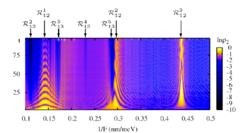
Figure 3: (Color online) Absolute occupancy function map for the second miniband in sample A; $\Psi(x,0)=w_{1}(x)$.

A typical case of interminiband carrier dynamics is illustrated in Fig. 3. The time evolution of $\rho_{\nu}(t,F)$ is shown on a map plot comprising results from a large number of time-dependent simulations over the range of bias $\frac{1}{F}=0.1\ldots 0.5~{}\frac{\textrm{nm}}{\textrm{meV}}$ with the step 1 $\frac{\textrm{nm}}{\mu\textrm{eV}}$; a greater value of $\rho(x,t)$ is shown in a lighter color. The large uniformly shaded areas correspond to exponential Zener decay of the wavepacket out of the superlattice potential. The darker vertical stripes originate from resonant Zener tunneling where the wavepacket decays extremely quickly at energy level anticrossings. In the TB approximation, the $n^{th}$ anticrossing between WSL$\mu$ and WSL$\nu$ occurs when the condition $E_{\nu}-E_{\mu}=F_{n}\,nd\equiv F_{1}\,d$ is satisfied Shimada et al. (2004b). In Fig. 3, the period in $\frac{1}{F}$ of the series of stripes marked on top by shorter arrows implies interminiband separation $F_{1}\,d=(223\pm 5)$ meV and clearly corresponds to the anticrossings associated with $\mathcal{R}_{13}$, since $E_{3}-E_{1}=227.2$ meV from our TB calculations.

$\mathcal{R}_{13}$ do not show strong Rabi oscillations, since the energy gap following the third miniband, $\Delta E_{3}$, is only 50 meV while an electron easily overcomes the interminiband separation $E_{2}-E_{1}=89$ meV. Therefore $\Delta E_{3}$ is too small to strongly bind an electron in the superlattice. On the other hand, $\Delta E_{2}=73.02$ meV suppresses tunneling to the third miniband at lower biases, and only $\mathcal{R}_{13}^{k\leq 5}$ are seen.

There is also a set of prominent periodic spikes marked by longer arrows, corresponding to the group of resonances $\mathcal{R}_{12}^{1\ldots 3}$. In contrast to $\mathcal{R}_{13}$, the resonances $\mathcal{R}_{12}$ do exhibit oscillations in $\rho_{2}(t)$ with time, corresponding to interminiband Rabi oscillations; they are wider and demonstrate a higher RZT rate for lower indices. The values $F_{\mathcal{R}_{12}^{2}}$=(6.9$\pm$0.2) $\frac{\textrm{meV}}{\textrm{nm}}$ and $F_{\mathcal{R}_{12}^{3}}$=(2.33$\pm$0.05) $\frac{\textrm{meV}}{\textrm{nm}}$ are reasonably close to the anticrossing calculated in Hino et al. (2005) (7.2 $\frac{\textrm{meV}}{\textrm{nm}}$ and 2.4 $\frac{\textrm{meV}}{\textrm{nm}}$, respectively), even though the potential considered here was not exactly the square barrier one used in that work.

Minor periodic changes in $\rho_{2}(t)$, creating a light horizontal mesh on the background with period $T_{B}$, are the signature of Bloch oscillations. For extremely high fields ($F>10~{}\frac{\textrm{meV}}{\textrm{nm}}$) the period and magnitude of these oscillations explodes (see e.g. the left edge of Fig. 11), since $\Delta E_{1}<F(d-a)$ and a transition to the next higher miniband can be made without tunneling; then a theory different from interwell hopping must be applied.

Generally, it was found that energy anticrossings do not necessarily result in strong RZT for a strongly bound interacting WSL. Rabi oscillations appear to be the reverse side of RZT in the WSL interaction: for strong RZT, overdamped Rabi oscillations are seen (i.e. $\mathcal{R}_{13}$ in the above example), while persistent and strong Rabi oscillations correspond to weak RZT (e.g. $\mathcal{R}_{12}$). A quantitative relation between the two depending on the strength of the potential and resonance index remains an open question; up to now Rabi oscillations have been studied separately from RZT.

III.1 Resonance shapes

The detailed structure of a resonance is shown in Fig. 4 which is an enlargement of the resonance $\mathcal{R}_{12}^{3}(A)$ from Fig. 3. Near a resonance, one sees Rabi oscillations as persistent oscillations of significant magnitude in $\rho_{2}(t)$ with period $T_{\mathcal{R}}\sim\,10\ldots 100\,T_{B}$ (the corresponding frequency range is between the microwave and infrared regions). Both vertical and horizontal cross-sections of the plot demonstrate periodic oscillations of $\rho_{2}$.

Figure 4: (Color online) Detailed view of $\mathcal{R}_{12}^{3}$ in sample A (top left). Period of Rabi oscillations vs. bias for $\mathcal{R}_{12}^{3}(A)$ is fitted by means of a Lorentzian as in Eq. 4 (top right). Relative occupancy functions and wavepacket norm are shown for the bias $F$ such that $|\frac{1}{F}-\frac{1}{F_{\mathcal{R}_{12}^{3}}}|=1.5\ \Gamma_{\mathcal{R}_{12}^{3}}$; $\rho_{1}$ is shown in solid (red), $\rho_{2}$ in dashed (green), $\rho_{3}$ in dotted (blue), $\rho$ in chain-dotted (magenta) lines, and asymptotic occupancy values in horizontal lines (bottom).

A vertical cross-section of $\mathcal{R}_{12}^{3}(A)$ at a near-resonant bias, shown at the bottom of Fig. 4, explicitly demonstrates Rabi oscillations. Oscillations in $\rho_{1}(t)$ and $\rho_{2}(t)$ are shifted in phase by $\pi$, which means that their coupling shows up as Rabi oscillations rather than RZT. In the example $\mathcal{R}_{12}^{3}(A)$, the third miniband contributes little to total wavepacket norm. Its population could be due to two factors: (i) the non-TB WS functions of the second miniband involve harmonics from the third TB miniband, and (ii) the escaping part of the wavepacket passing through the third miniband on its way to the continuum. Since $\rho_{3}(t)$ oscillates in phase with $\rho_{2}(t)$, we conclude that the second factor is dominant in this example.

When the asymptotic values of $\rho_{1}(t)$ and $\rho_{2}(t)$ in the limit $t\rightarrow\infty$ are not equal, as in the bottom panel of Fig. 4, we are dealing with a so-called asymmetric decay Fidio and Vogel (2000): the minibands 1 and 2 are coupled to the continuum to a different extent. Right at a resonance bias value, the extremely strong interaction between the two minibands essentially merges them, and their asymptotic population values were both very close to ${1}/{2}$. Away from the resonant bias, the coupling is weaker and the difference between the two values increases, eventually approaching unity.

The dynamics of $\Psi(x,t)$ in k-space demonstrates features similar to those of Bloch oscillations across a single miniband, i.e. most of the wavepacket steadily traverses the first and the second minibands as a whole with period $2\,T_{B}$ as shown in Fig. 5. The map plot consists of a series of images of the total probability density $\rho(x,t)$. We chose $\Psi(x,0)$ to be a linear combination of two Wannier functions in order to reduce the wavepacket uncertainty in k-space and to get a better resolution of fine details. From this perspective, an anticrossing can be thought of as a phenomenon of two adjacent WSL merging into a single broader one.

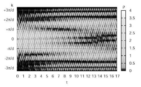
Figure 5: (Color online) Dynamics of the wavepacket having initial form $\Psi(x,0)=w_{1}(x)+w_{1}(x+3d)$ in reciprocal space at $\mathcal{R}_{12}^{2}(A)$.

For all resonance indices and samples examined, the Rabi oscillation period $T_{\mathcal{R}}$ of an $n^{th}$ resonance clearly showed a Lorentzian-like dependence as anticipated from the nature of Rabi oscillations Akulin and Karlov (1992):

$$T_{n}(F) = T_{n}^{max}\,\Bigg{[}\bigg{(}\frac{\frac{1}{F}-\frac{1}{F_{\mathcal{R}_{\nu\mu}^{n}}}}{\Gamma_{\mathcal{R}_{\nu\mu}^{n}}}\bigg{)}^{2}+1\Bigg{]}^{-\frac{1}{2}}$$ (4)

which is shown in the top right panel of Fig. 4. The data were obtained from a fit of $\rho_{2}(t)$ at $\mathcal{R}_{12}^{3}(A)$ over a long length of time considered ($t=50\ldots 100~{}T_{\mathcal{R}}$). When speaking of half-width at half-maximum (HWHM, or $\Gamma_{\mathcal{R}_{\mu\nu}^{n}}$), we will be referring to HWHM of the corresponding fit to $T_{n}(F)$ at $\mathcal{R}_{\mu\nu}^{n}$.

The maximum Rabi oscillation period observed at a resonant bias, $T_{n}^{max}$, was found to grow exponentially with resonance index $n$ in the following way:

$$T_{n}^{max} = T_{1}^{max}\bigg{(}\frac{T_{2}^{max}}{T_{1}^{max}}\bigg{)}^{(n-1)},\;\;\;n=1,2,\ldots$$ (5)

(see left part of Fig. 6), which was expected Glück et al. (2000) since the transition matrix element $|\langle W_{1}^{k}(x)|W_{2}^{m}(x)\rangle|^{2}\,~{}\propto~{}e^{-|k-m|}$. As the bias is reduced, the horizontal tunneling channel to the next WSL lengthens, and it takes longer for the probability density to build up in the other miniband. We remark that perturbation theory predicts the dependence in Eq. (5) to be linear Diez et al. (1998), but that does not apply at the high bias considered.

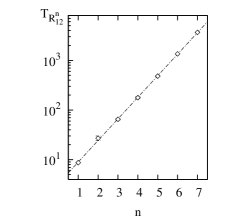
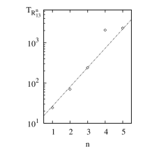
Figure 6: Logarithmic fit of $T_{n}^{max}$ versus resonance index $n$ for $\mathcal{R}_{12}(A)$ (left) and $\mathcal{R}_{13}^{n}(C)$ (right).

III.2 Pulsed output from the system

Rabi oscillations of the carrier produce a periodic coherent pulsed output with period $T_{\mathcal{R}}$ similar to that of Bloch oscillations Glück et al. (2002a). The data shown in Fig. 7 correspond to a record of $|\Psi_{end}|^{2}~{}\equiv~{}|\Psi(x_{end},t)|^{2}$ values over time, at the endpoint $x=x_{end}$ of the superlattice having a lower saturation potential.

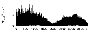
Figure 7: Pulsed output of a Rabi oscillating system at $\mathcal{R}_{12}^{3}(A)$ (top) and $\mathcal{R}_{13}^{4}(C)$ (bottom); chain-dotted line is the wavepacket norm.

In the case of a relatively short Rabi oscillation period, the output consists of damped sinusoidal oscillations decaying at the same rate as the wavepacket norm. For a long Rabi oscillation period accompanied by weak RZT, as in the case of $\mathcal{R}_{13}^{4}(C)$, the pulsed output is significantly distorted. Over the course of a single oscillation, the net effect of relatively small factors becomes significant; in the bottom section of Fig. 7, Rabi oscillations cause the drops in $|\Psi_{end}|^{2}$ with period $T_{\mathcal{R}}=2050~{}T_{B}=186~{}ps$. Away from a resonance, the output pulses flatten out and on, a time scale longer than $T_{B}$, only a smooth exponential decay in accordance with Zener theory would be observed.

The form of the pulsed output is determined by the strength of Rabi oscillations, by their rate of magnitude decay, and by the strength of RZT. In principle, one could experimentally observe Rabi oscillations as well as establish the relation between Rabi oscillations and RZT, by measuring the system’s pulsed output.

IV Wavepacket self-interference

A detailed consideration of the interference mechanism allows us to analyze resonance phenomena and draw some important conclusions without the need to calculate the system’s spectrum.

A strong correlation between subsequent well-to-well tunneling events arises due to their coherence. This correlation manifests itself in the interference between Bloch oscillations and intrawell oscillations (first resolved in Bouchard and Luban (1995)) with frequencies $\omega_{B}$ and $\omega_{\mu\nu}$ that is constructive for near-resonant bias and destructive otherwise, with frequency detuning per single intrawell oscillation cycle

$$\Delta\omega\,=\,\omega_{\mu\nu}-n\omega_{B} = \frac{(E_{\mu}-E_{\nu})-Fnd}{\hbar}$$ (6)

around a resonance with index $n$. If constructive, the interference leads to a gradual transition of the center of mass of probability density between the 0^th and the $n^{th}$ cells and between the $\mu^{th}$ and the $\nu^{th}$ Brillouin zones in k-space.

Figure 8: Dynamics of the electron dipole moment $\langle\Psi(x,t)|x|\Psi(x,t)\rangle$ calculated over the 0^th (solid line) and the second (dashed line) cells at $\mathcal{R}_{12}^{2}(A)$. the wavepacket $\Psi(x,0)=w_{1}(x)$ was taken at a near-resonant bias so that $\frac{T_{\mathcal{R}}}{2}=13.5~{}T_{B}$ ($\frac{1}{F}=0.296~{}\frac{\textrm{nm}}{\textrm{meV}}$, $\frac{1}{F}-\frac{1}{F_{\mathcal{R}_{12}^{2}}}$ = 0.8 $\Gamma_{\mathcal{R}_{12}^{2}}$); position $n$ is taken with respect to the center of the corresponding cell, in units of the cell width.

At a resonant bias, the saturation value of occupancy functions of the two coupled minibands approached unity. Off resonant bias, the transition of probability density from one miniband to another was observed to reverse direction when a dephasing of $\pi$ had accumulated between the two resultant oscillations of wavepacket components residing in the two coupled minibands (Fig. 8). One can clearly see intrawell oscillations (especially around $t=0$) and Bloch oscillations, as well as the process of dephasing between Bloch and intrawell oscillations. If we call the wavepacket piece residing in the $n^{th}$ cell $\Psi_{n}$, then with time, the phase shift between the peaks of the resultant oscillatory motion of $\Psi_{0}$ and $\Psi_{2}$ builds up, and reaches a net increment of $\pi$ at $t=\frac{T_{\mathcal{R}}}{2}=13.5~{}T_{B}$. Remarkably, this interval corresponds to a maximum of $|\Psi_{2}(t)|^{2}$ and hence to a Rabi oscillation peak.

Given these results, we conclude that interminiband Rabi oscillations are governed by the process of self-interference of a wavepacket subject to two intrinsic frequencies: $\omega_{B}$ and $\omega_{\mu\nu}$, and the amplitude of Rabi oscillation at a given bias is determined by bias detuning from its resonant value. This again illustrates the coherence of multiwell tunneling, and in principle one can judge the coherence length of a superlattice by the number of observable resonances.

IV.1 Built-up state

Figure 9: Comparison of norms of a built-up state at $F_{\mathcal{R}_{12}^{2}(A)}$ at resonant field for $\Psi(x,0)=w_{1}(x)$ (dashed line) and $\Psi(x,0)=W_{1}(x)$ (dotted line) with the corresponding Wannier-Stark state at $\mathcal{R}_{12}^{3}(A)$ (solid line line) in the left panel. In the right panel, the built-up state at a near-resonant bias is in dotted line. For reference, the biased superlattice potential is shown in double-dotted line.

Let us consider the shape of the probability density that is building up, away from the wavepacket’s original location, in the process of Rabi oscillation (built-up state). Without loss of generality, we will consider dynamics of $\Psi(x,0)=w_{1}(x)$ at $\mathcal{R}_{12}(A)$ and will denote by $\Psi_{\mathcal{R}}(x)$ a built-up state in the corresponding cell $n$. The shape of the probability density $|\Psi_{\mathcal{R}}(x)|^{2}$, turns out to be nearly the same for different values of the off-resonance field, and it also closely resembles the corresponding TB WS wavefunction, at least when $|\Psi_{\mathcal{R}}(x)|^{2}$ is at its peak.

The latter comparison is made in the left panel of Fig. 9. Although in Hino et al. (2005) the corresponding computed resonant wavefunction had significant presence in the wells with indices $n=-3\ldots-7$, our $|\Psi_{\mathcal{R}}(x)|^{2}$ is not large there. A possible explanation is that the built-up state in the second miniband may include components from the third miniband as well. $\Psi_{\mathcal{R}}(x)$ appears to be only slightly more widespread than the TB $W_{2}(x)$, and on a linear plotting scale they are quite close as expected from Glück et al. (2002a) for the moderate field considered. Note also that $|\Psi_{\mathcal{R}}(x)|^{2}$ shows slight asymmetry in k-space, in agreement with Glück et al. (2002a): for example, in Fig. 5 at $t=\frac{T_{\mathcal{R}}}{2}=13.5~{}T_{B}$, there is more probability density present at negative values of $k$ than at positive ones. This tells us that at moderate fields there is a great similarity between true and TB WS states. For comparison, the results for $\Psi(x,0)=W_{1}(x)$ are presented as well. Despite dissimilar shapes of the initial forms $W_{1}(x)$ and $w_{1}(x)$, the built-up state looks almost the same for both.

The built-up states at resonant and off-resonant values of bias at $\mathcal{R}_{12}^{2}$ are compared in the right panel of Fig. 9. The first one was taken at $F$ such that the saturation population of the second miniband was $\rho_{2}=0.77$ ($\frac{1}{F}-\frac{1}{F_{2}}=0.5~{}\Gamma_{2}$). The second built-up state was taken at $F=F_{2}$ at the moment when the population of the second miniband reached the same value $\rho_{2}=0.77$. Their close resemblance reveals that over the range of near-resonant fields, the build-up mechanism of $|\Psi_{\mathcal{R}}(x)|^{2}$ is the same and produces a (rescaled) WS state of the second miniband at a resonant bias.

IV.2 Resonance condition

In the process of Bloch oscillatory motion, the wavepacket tunnels out whenever it approaches the end of the Bloch oscillatory domain, producing a leaking out pulse. As a pulse propagates in space upon its escape, it scatters on the potential barriers, and some fraction of a pulse stays trapped in cells outside of the initial one. If the oscillations of the trapped part of a pulse happen to be in phase with those of a subsequent incoming pulse, the conditions for constructive interference are met and the probability density $|\Psi_{\mathcal{R}}(x)|^{2}$ builds up in this well.

For realistic fields, $\omega_{B}<\omega_{\mu\nu}$ (or $T_{B}>T_{\mu\nu}$), and in order for oscillations of two subsequent pulses to be in phase in the $n^{th}$ well, the equality

$$n = \frac{T_{B}}{T_{\mu\nu}}\,=\,\frac{\omega_{\mu\nu}}{\omega_{B}}$$ (7)

must be satisfied: this is the condition for a resonance with index $n$. A gradual decrease in bias makes $\omega_{B}$ smaller, thus increasing $n$ and shifting the location of the built-up state further down the potential ramp. Provided that $\hbar\omega_{\mu\nu}~{}\equiv~{}E_{\nu}-E_{\mu}$ and $\hbar\omega_{B}~{}\equiv~{}F_{n}\,d=\frac{F_{1}}{n}d$, for a resonance to occur between the $\nu^{th}$ and the $\mu^{th}$ minibands, $n=\frac{E_{\mu}-E_{\nu}}{F_{n}d}$. In the TB approximation ($E_{\mu}$ and $E_{\nu}$ are independent of $F$), that leads to a well-known result $F_{n}\,\propto\,\frac{1}{n}$ Shimada et al. (2004b). This relation is satisfied surprisingly well as indicated by results in the following subsection.

From the above argument, it follows that the role of the interband jumping mechanism, as proposed in Fidio and Vogel (2000) for Rabi oscillation dephasing, must be minimal. Indeed, once tunneling of the carrier into a certain well (and reflection back which doubles the phase increment of the $\psi_{n}(x,t)$) puts it out of phase with the rest of the system, such well will not be largely populated due to destructive interference. Mathematically, the discrete bias values allowing constructive self-interference correspond to existence of poles of the system scattering matrix, which can be employed to successfully build a WS state for a multiband system Glück et al. (2002b).

IV.3 Resonant bias values

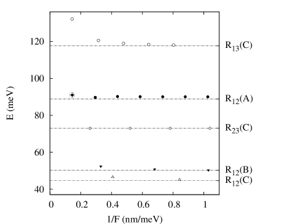
Figure 10: Values of $F_{\mathcal{R}_{\mu\nu}^{n}}nd\$ plotted versus inverse bias for various resonances with lowest indices ($n\,=\,1,2,3,\ldots$ ascending from the left to the right) and compared with interminiband separation $E_{\mu}-E_{\nu}$ calculated from the tight-binding model. Filled circles mark the data corresponding to $\mathcal{R}_{12}(A)$, filled triangles to $\mathcal{R}_{12}(C)$, empty circles to $\mathcal{R}_{13}(C)$, empty rhombi to $\mathcal{R}_{23}(C)$, empty triangles to $\mathcal{R}_{12}(B)$.

In order to check the validity of TB model calculations for predicting resonant bias values at high fields, in Fig. 10 the values of $nd\,F_{n}$ obtained from our simulations for the first few resonances in different samples are compared with the corresponding interminiband separations calculated in the TB approximation, using a Kronig-Penney model. The data are plotted versus $\frac{1}{F}$; $x$-error bars for all points refer to HWHM of a given resonance $\Gamma_{n}$, whereas $y$-error bars show broadening of the energy levels and equal $\Gamma_{n}$ rescaled in the same manner as $\frac{1}{F_{n}}$, i.e. $nd\,\Gamma_{n}$.

Excluding $\mathcal{R}_{13}(C)$, the difference between the de facto relative position of the energy levels found as $F_{\mathcal{R}_{\mu\nu}^{n}}nd$ and that from the TB calculations ($E_{\mu}-E_{\nu}$), is less than 2 meV or $\leq$ 5%, for the resonances depicted. This is true even for resonances between non-ground minibands $\mathcal{R}_{23}^{k<4}(C)$ (this type of resonance has experimentally been observed in Fidio and Vogel (2000)). Thus even at high fields the equality $F_{\mathcal{R}_{\mu\nu}^{n}}nd=E_{\nu}-E_{\mu}$ holds reasonably well, and the resolved resonances occur periodically in $\frac{1}{F}$. However, in many cases this difference is seen to be much larger than the corresponding HWHM which cannot be explained by broadening of the transition line alone. Because $F_{\mathcal{R}_{\mu\nu}^{n}}nd$ is always larger than $E_{\mu}\,-\,E_{\nu}$ and this difference increases with bias, it must be a result of stronger coupling to the continuum at higher bias. This effect is similar to the energy level structure of a potential well becoming sparce as the well becomes shallower.

Unlike other resonances, for the series $\mathcal{R}_{13}(C)$ the value of $nd\,F_{n}$ departs significantly from $E_{3}-E_{2}$ for $\frac{1}{F}\lesssim 0.4~{}\frac{\textrm{nm}}{\textrm{meV}}$. It has been verified that this deviation is not due to extreme narrowness of the first miniband in sample C. As follows from the series $\mathcal{R}_{23}(C)$, the mutual alignment of levels belonging to WSL2 and WSL3 is almost unchanged up to $\frac{1}{F}\gtrsim 0.25$; so it is the change in mutual arrangement of WSL1 and WSL2 that is driving this deviation.

The threshold value $\frac{1}{F}\approx 0.4~{}\frac{\textrm{nm}}{\textrm{meV}}$ corresponds to the potential drop per cell $Fd\approx 47.4$ meV which is close to the interminiband separation $E_{2}-E_{1}=44.6$ meV. According to the TB model, at $\frac{1}{F}\lesssim 0.4~{}\frac{\textrm{nm}}{\textrm{meV}}$ the energy levels $E_{1}^{0}$ and $E_{2}^{1}$ would be found in the same cell. This is clearly impossible due to the Pauli exclusion principle, hence, the structure of separate Wannier-Stark ladders is completely destroyed at this point. At such bias, the $w_{\nu}(x)$ correspond only to the set of Fourier components with certain wavelengths rather than wavefunctions belonging to certain minibands.

Disruption of the WSL structure seems not to affect $\mathcal{R}_{23}(C)$, however: the initial wavepacket $\Psi(x,0)=w_{2}(x)$ having only components with wavelength $\lambda\in[\frac{d}{2},d]$ was noticed not to gain any significant components with $\lambda\in[d,2d]$ over time in our simulations, because of conservation of energy. In general, the structure and properties of $\mathcal{R}_{23}$ were found to be similar to those of $\mathcal{R}_{12}$, at any bias.

V Resonance across three minibands

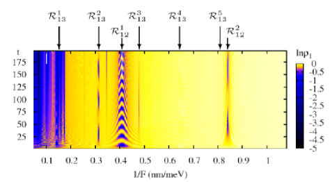
Figure 11: (Color online) Absolute occupancy function map for the first miniband in sample C; $\Psi(x,0)=w_{1}(x)$.

In a strong potential (sample C) having well-isolated minibands, we were able to resolve $\mathcal{R}_{13}^{2\ldots 5}(C)$; the location of several first resonances is indicated with longer arrows in Fig. 11. To our knowledge, the phenomenon of Rabi oscillations across three minibands has been neither observed nor simulated before.

Dynamics of Rabi oscillations at $\mathcal{R}_{13}^{3}$ shows that the wavepacket resides mostly in the first and the third minibands. In real space (upper panel of Fig. 12; $\rho_{\nu}(t)$ is seen as a part of $\rho(x)$ whose shape has $\nu$ humps per cell), there is little probability residing in wells -1 and -2 at all times. In reciprocal space (lower panel), the second Brillouin zone consistently remains underoccupied relative to the first and third zones; some traces of $\rho(k,t)$ in the fourth and the fifth Brillouin zones correspond to RZT, and the finer background oscillations are caused by Bloch oscillations in individual minibands. Thus, the carrier mostly bypasses the second miniband since the resonance condition for $\mathcal{R}_{12}$ is not well satisfied, and tunnels directly into the third miniband.

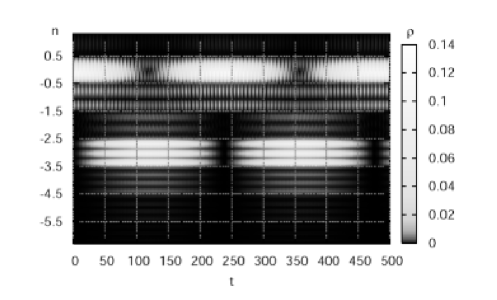
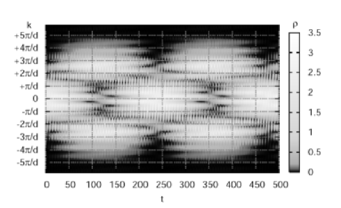
Figure 12: (Color online) Dynamics of the wavepacket $\Psi(x,0)=w_{1}(x)$ in real (top) and reciprocal (bottom) space at $\mathcal{R}_{13}^{3}$ in sample C.

It was found that $\mathcal{R}_{12}$ and $\mathcal{R}_{13}$ have many features in common. Namely, the resonance shape was similar, the oscillations of $\rho_{1}(t)$ were close to sinusoidal, Eq. (4) was satisfied, and in k-space most part of a wavepacket $\Psi(x,0)=w_{1}(x)$ traversed the first three Brillouin zones of the TB model ($k\in[-\frac{3\pi}{d},\frac{3\pi}{d}]$) as a whole. However, individual intrawell oscillations were not well pronounced at $\mathcal{R}_{13}$ because of the strong potential barriers in sample C and the fact that intrawell oscillations between the pairs of coupled minibands 1$\leftrightarrow$2 and 1$\leftrightarrow$3 are of comparable magnitude and strongly interfere with each other, as was noticed from the irregular shape of the resulting oscillations of a wavepacket within the 0^th cell. Also, within the 0^th cell, the center of the resultant oscillations of the probability density was shifted down the potential ramp from the center of the cell, under the influence of strong bias which creates asymmetry about the cell center.

V.1 Role of sandwiched miniband

For a resonance across three minibands, an exponential fit based on the two-miniband approximation is not a good fit to $T_{n}^{max}\,(n)$ any more (right panel of Fig. 6). The reason lies in the involvement of the second miniband which is “sandwiched” between minibands 1 and 3, in the interminiband tunneling process. Despite its small average population value, the second miniband must be taken into account at any bias as will be shown below.

The role of the second miniband in carrier transfer between minibands 1 and 3 must depend on resonance index, $n$. Otherwise, $\langle\rho_{2}(t)\rangle$ should be proportional to the interminiband tunneling rate of $\Psi(x,t)$, or inversely proportional to the period of Rabi oscillations, and the latter would be described by Eq. (5). Hence, this would imply $\langle\rho_{2}\rangle\>\propto e^{-n}$.

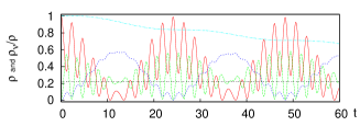
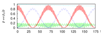
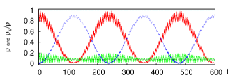
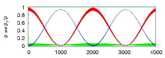
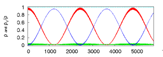
Figure 13: (Color online) Occupancy functions and wavepacket norm at $\mathcal{R}_{13}^{n}(C)$ for $n$ = 1 (top) through 5 (bottom). $\rho_{1}$ in solid (red), $\rho_{2}$ in dashed (green), $\rho_{3}$ in dotted (blue)and $\rho$ in chain-dotted (magenta) lines; the broken black line shows $\langle\rho_{2}\rangle$.

Values of $\langle\rho_{2}\rangle$ obtained are shown in Fig. 13, which displays dynamics of the relative occupancy function at $\mathcal{R}_{13}(C)$. It is remarkable that, despite the strong coupling to the third miniband, the RZT rate is small for the resonance indices $n>2$ thus allowing for long-lasting Rabi oscillations. For lower resonance indices, the population of the second miniband reaches significant level at certain times. As the resonance index ascends, the average population of the second miniband at $\mathcal{R}_{13}^{n}$ decreases (Fig. 13); its population is largely caused by Rabi oscillations between minibands 1 and 3. As $\rho_{2}(t)\rightarrow 0$, most of the wavepacket undergoes sinusoidal oscillations between minibands 1 and 3, i.e. for lower biases the interminiband dynamics resembles a two-miniband model (which would assume $\rho_{2}(t)\equiv 0$). The values of $\langle\rho_{2}\rangle$ are shown separately in Fig. 14 and appear to significantly deviate from exponential dependence at $\mathcal{R}_{13}^{4}$.

In the process of Rabi oscillations at $\mathcal{R}_{13}$, the population level of the sandwiched second miniband is higher, the better is the match in energy between the states from WSL2 and the initial carrier energy $E_{1}^{0}$. The reason lies in the tunneling mechanism involved: in the process of the multiwell tunneling between minibands 1 and 3, an electron’s energy after a certain number of interwell hops can be close to $E_{2}$. This proximity greatly enhances population of the sandwiched miniband by providing available density of states. Conversely, a large population level of a sandwiched miniband favors transition between the first and the third minibands. When the transition element $x_{12}^{02}\,x_{23}^{25}$ becomes comparable to $x_{13}^{05}$ (here $x_{\nu\mu}^{mn}\equiv\langle w_{\nu}^{n}(x)|x|w_{\mu}^{m}(x)\rangle$), indirect tunneling through the sandwiched miniband becomes significant. Therefore the degree of participation of the second miniband and its effect on $\mathcal{R}_{13}$ is determined by alignment of energy levels in WSL1, WSL2 and WSL3 and is dissimilar for resonances with different indices. The details of the influence of this alignment on the electron dynamics will be given in the next subsection V.2.

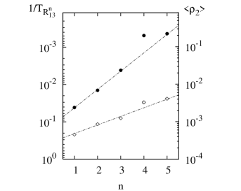
Figure 14: Rabi oscillation frequency (left scale, filled circles) and $\langle\rho_{2}\rangle$ (right scale, empty circles) at $\mathcal{R}_{13}(C)$ fitted with exponential curves (chain-dotted lines) on a logarithmic scale.

The correlation between coupling strength to the sandwiched miniband and the rate of interminiband transition, or Rabi oscillation frequency, is clearly demonstrated in Fig. 14: for $\mathcal{R}_{13}^{4}$, both $\frac{1}{T_{\mathcal{R}}}$ and $\langle\rho_{2}\rangle$ are smaller than expected from the exponential fit. For index $n=4$, the tunneling channel between the levels $E_{1}^{0}$ and $E_{3}^{4}$ consists of four interwell hops, and the intermediate energy levels available to the carrier are $E_{2}^{1,2}$. In this case, the alignment of $E_{2}^{1,2}$ turns out to be particularly unfavorable for them to act as a strong transition channel. At $F=F_{4}=1.245~{}\frac{\textrm{nm}}{\textrm{meV}}$, $E_{2}^{1}$ and $E_{2}^{2}$ are equally remote from the carrier’s initial energy: $|E_{1}^{0}-E_{2}^{1}|\approx|E_{1}^{0}-E_{2}^{2}|$$\approx\frac{F_{4}d}{2}\approx 20$ meV (whereas in the other cases, when $n\neq 4$ and $n>1$, one of the levels $E_{2}^{k}$ is closer to $E_{1}^{0}$ than 7 meV). Such an alignment can also be anticipated from Fig. 11, where $\mathcal{R}_{13}^{4}$ lies in the middle between $\mathcal{R}_{12}^{1}$ and $\mathcal{R}_{12}^{2}$ and hence is particularly isolated from any of the $\mathcal{R}_{12}^{k}$.

A sandwiched miniband affects not only Rabi oscillations, but also RZT. In Fig. 3, we can see that despite a weaker bias, RZT at $\mathcal{R}_{13}^{5}$ is stronger than for the preceding $\mathcal{R}_{13}^{4}$ for the same reason, namely proximity to $\mathcal{R}_{12}^{2}$. There, it also makes Rabi oscillations corresponding to $\mathcal{R}_{12}$ vanish at the given field since the barrier through which the carrier tunnels to the third miniband and then to the continuum is significantly reduced by coupling between WSL2 and WSL3. In other words, closely situated resonances mutually influence each other and can be referred to as coupled resonances.

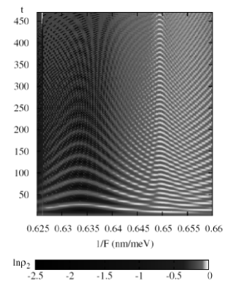
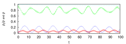
Figure 15: (Color online) Detailed view of coupled resonances ($\mathcal{R}_{12}^{2}$,$\mathcal{R}_{23}^{3}$ and $\mathcal{R}_{13}^{5}$) in sample B for $\Psi(x,0)=w_{2}(x)$. Relative occupancy functions dynamics at bias $\frac{1}{F}$=0.646 $\frac{\textrm{nm}}{\textrm{meV}}$ is shown in the bottom panel; $\rho_{1}$ is shown in solid (red), $\rho_{2}$ in dashed (green), $\rho_{3}$ in dotted (blue), and $\rho$ in chain-dotted (magenta) lines.

Despite the sometimes small value of its average population, the second miniband has a significant effect on resultant interminiband dynamics. Thus to calculate parameters of a resonance across three minibands, it is necessary to take at least these three minibands into consideration.

V.2 Coupled resonances

In order to understand the interaction between different resonances better, let us consider an example where strength of interminiband coupling for different resonances is comparable and the resonances strongly interfere with each other. The region corresponding to the coupling of two resonances $\mathcal{R}_{23}^{3}$ and $\mathcal{R}_{12}^{2}$ in sample B is shown in Fig. 15, a map plot of $\rho_{2}$ for $\Psi(x,0)=w_{2}(x)$. $\mathcal{R}_{12}^{2}$ is situated on the left and $\mathcal{R}_{23}^{3}$ on the right, the former being wider due to its lower resonance index.

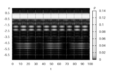
Figure 16: (Color online) Dynamics of the wavepacket $\Psi(x,0)=w_{1}(x)$ in direct space in the coupled resonances zone in sample B.

Detail of the carrier dynamics for field $\frac{1}{F}$=0.646 $\frac{\textrm{nm}}{\textrm{meV}}$ where contributions from $\mathcal{R}_{12}^{2}$ and $\mathcal{R}_{23}^{3}$ are nearly equal, are shown in the bottom section of Fig. 15. Since all three minibands are interacting at the same time, the resultant dipole dynamics looks somewhat similar to a superposition of the three corresponding Rabi oscillations for the individual resonances ($\mathcal{R}_{12}^{2}$, $\mathcal{R}_{23}^{3}$ and $\mathcal{R}_{13}^{5}$), and the time evolution of $\rho_{1,2,3}(t)$ exhibits beats. Therefore for coupled resonances, the resultant Rabi oscillations are an interference product of not only Bloch and intrawell oscillations, but also of Rabi oscillations corresponding to the other pairs of strongly coupled minibands in the sample. This interference allows the carrier to use the “extra” density of states to enhance tunneling. A map plot of the wavefunction in the coupled resonances zone (Fig. 16) demonstrates that large miniband populations facilitate the build-up of each another. For example, $\rho_{2}(t)$ is relatively low at $t=35~{}T_{B}$ and $t=70~{}T_{B}$, i.e. at the moments when $\rho_{3}(t)$ is almost zero. Likewise when $\rho_{2}(t)$ is relatively large, $\rho_{3}(t)$ becomes larger as well (e.g. at $t=20~{}T_{B}$, 50 $T_{B}$ and 90 $T_{B}$).

Obviously the two-miniband model cannot reproduce such behavior. As was recently found Villas-Boas et al. (2005), Rabi oscillations in a three-level system are not merely a summation of Rabi oscillations between the three separate pairs of minibands, they rather are a coherent superposition. In fact, the temporary reduction of Rabi oscillation amplitude observed in work Fan et al. (2001) was due to Rabi oscillation revival, i.e. the beats caused by superposition of Rabi oscillations between several lowest minibands, rather than to Rabi oscillation dephasing.

VI Conclusion

In conclusion, our time-dependent simulations of electron dynamics in a biased superlattice provide an overview of carrier behavior over a large range of bias. We were able to identify energy level anticrossings as resonances displaying Rabi oscillations and/or RZT and to study the structure of these resonances in detail; our findings could be experimentally studied by observing the system’s pulsed output.

It has been shown that Rabi oscillations result from constructive interference between Bloch and intrawell oscillations. A distinct interminiband resonance occurs whenever the initial wavepacket is capable of building up a Wannier-Stark state of significant magnitude away from its initial location, through the coherent process of self-interference.

We have also reported and analyzed Rabi oscillations across three minibands. The important role of a sandwiched miniband in the transitions across more than one miniband has been studied: energy-wise it provides available density of states in the intermediate tunneling region, and dynamically it invokes additional Rabi oscillations interfering constructively with the principal interminiband transition.

At a resonance across three minibands and in the coupled resonances region, the resultant carrier dynamics has significant contribution from all three minibands. Hence these cases cannot be described within the commonly used two-miniband model, and require taking at least three minibands into consideration.

Interminiband separations calculated in the tight-binding approximation can be used to predict resonant values of bias in the high-field regime with reasonable accuracy for a variety of potentials, including resonances between minibands 2 and 3 and those across three minibands (e.g. $\mathcal{R}_{13}$, with the only restriction $Fd<E_{2}-E_{1}$).

Although the present work focuses on an ideal zero-temperature superlattice under uniform constant electric field, the numerical methods utilized are easily capable of handling time-dependent irregular potentials. With minor variations, the numerical techniques can be applied to study carrier dynamics in other systems (e.g. double quantum dots Roskos et al. (1992); Leo et al. (1991) and irregularly shaped potentials Diez et al. (1996)) and even areas of physics, such as photonics Ghulinyan et al. (2005); Malpuech et al. (2001); Paulau and Loiko (2005); Wilkinson (2002) and cold atom optical traps Choi and Niu (1999); Konotop et al. (2005); Morsch et al. (2001); Kolovsky and Korsch (2006); these are reserved for the future investigations.

Appendix A Discrete transparent boundary conditions

Our numerical method was based on TrBC implemented with Numerov and Crank-Nicholson methods for space and time respectively, with the cumulative precision $\mathcal{O}((\delta x)^{5})$ in space and $\mathcal{O}((\delta t)^{2})$ in time. We extended the discrete TrBC as described in Moyer (2004) to the case of unequal saturation potentials on opposite sides. For the most part, we keep the same notation as in Moyer (2004).

Let us express Eq. (1) in terms of finite differences. We will start from the finite difference form of the system’s propagator which translates the time by $\delta t$

$$\Psi(x,t+\Delta) \approx e^{-iH(t)\Delta}\,\Psi(x,t)$$

with $\Delta\,\equiv\,\frac{\delta t}{\hbar}$ and $H(t)$ being the (possibly time-dependent) Hamiltonian of the system. Cayley’s approximation preserves unitarity and is exact to second order:

$$e^{-iH\Delta} = \frac{1-\frac{1}{2}\,i\,H\Delta}{1+\frac{1}{2}\,i\,H\Delta}\ +\ \mathcal{O}\big{(}\Delta^{3}\big{)}$$

A little algebra leads to the expression

$$\bigg{[}\frac{\partial^{2}}{\partial x^{2}}\,-\,\frac{2\,mm^{*}}{\hbar^{2}}\Big{(}V(x,t)-\frac{2i}{\Delta}\Big{)}\bigg{]}\,\Big{(}\Psi(x,t+\Delta)+$$

$$+\,\Psi(x,t)\Big{)}\ =\ \frac{8\,i\,mm^{*}}{\hbar^{2}\Delta}\,\Psi(x,t)\ +\ \mathcal{O}\big{(}\Delta^{3}\big{)}$$

with the notation $V(x,t)=V_{SL}(x)+xF$. It serves as a discretized in time version of Eq. (1) and as a starting point for discretization in space using the Numerov method.

In order to build the solution $\Psi(x,t)$ to Eq. (1), we will use a uniform space grid consisting of $J$ points and defined as $x_{j}=j\,\delta x,\ (j=0,1,\ldots,J-1)$ and uniform time grid $t^{(k)}=k\,\delta t,\ (k=0,1,\ldots)$. The subscript $j$ will refer to the inner points $x_{j}$, and $e$ to the end points $x_{0}$ or $x_{J-1}$ as appropriate; the superscript $(k)$ will denote the time instant $t^{(k)}$. Thus $\Psi(x_{j},t^{(k)})\equiv\Psi_{j}^{(k)}$ and $V(x_{n})\equiv V_{n}$.

To apply TrBC in the Numerov approximation for the 1D case, the necessary conditions are: $V(x<x_{0})=V(x=x_{0})\equiv V_{0}$, and $V(x>x_{J-1})=V(x=x_{J-1})\equiv V_{J-1}$, as well as $\Psi_{e}^{(0)}=0$ at both ends. Having started at $t=0$, we proceed as follows to construct $\Psi(x,t^{(k+1)})$ from $\Psi(x,t^{(k)})$:

(i) Calculate the time-independent coefficients over the space grid:

$$g_{j} = \frac{2\,mm^{*}}{\hbar}\,(V_{j}-\frac{2\,i}{\Delta})\ \ \ \ \ \ \ 0\leq j\leq J-1$$

$$d_{j} = 1-\frac{(\delta x)^{2}}{12}\,g_{j}\ \ \ \ \ \ \ \ \ \ \ \ \ \ 0\leq j\leq J-1$$

$$e_{j} = \left\{\begin{array}[]{ll}\alpha_{0}&\textrm{$j=0$}\\ 2+(\delta x)^{2}\,\frac{g_{j}}{d_{j}}-\frac{1}{e_{j-1}}&\textrm{$0<j<J-1$}\end{array}\right.$$ (10)

(ii) Calculate the time-independent border coefficients ($e=0$ or $J-1$ separately):

$$a_{e} = 1+\frac{(\delta x)^{2}}{2}\,\frac{g_{e}}{d_{e}}$$

$$\alpha_{e} = a_{e}+\sqrt{a_{e}^{2}-1}$$

$$c_{e} = 1-\frac{2\,i\,(\delta x)^{2}mm^{*}}{3\delta t}\,\frac{1}{d_{e}}$$

$$\phi_{e} = \arg\Big{(}\frac{a_{e}^{2}-1}{c_{e}}\Big{)}$$

$$A_{e} = \frac{1-|a_{e}|^{2}}{|1-a_{e}^{2}|}$$

$$\sigma_{e} = d_{e}(a_{e}-\alpha_{e})$$

$$\rho_{e} = d_{e}^{*}(a_{e}^{*}-\alpha_{e})$$

(iii) Construct the polynomials for the next time step:

$$P_{e}^{(k)} = \left\{\begin{array}[]{ll}1&\textrm{$k=-1$}\\ A_{e}&\textrm{$k=0$}\\ \frac{2k+1}{k+1}\,A_{e}P_{e}^{(k-1)}-\frac{k}{k+1}\,P_{e}^{(k-2)}&\textrm{$k>0$}\end{array}\right.$$ (14)

$$L_{e}^{(k)} = \left\{\begin{array}[]{ll}e^{-i\phi_{e}}\,P_{e}^{(k)}&\textrm{$k=0$}\\ \frac{1}{2k+1}\,e^{-i(k+1)\phi_{e}}\Big{(}P_{e}^{(k)}-P_{e}^{(k-2)}\Big{)}&\textrm{$k>0$}\end{array}\right.$$ (17)

(iv) Calculate the time-dependent coefficients over the space grid:

$$q_{j}^{(k+1)}=\left\{\begin{array}[]{ll}\rho_{0}\Psi_{0}^{(k)}+\sigma_{0}\sum^{k}_{m=0}\,L_{0}^{(k-m)}\Psi_{0}^{(m)}&\textrm{$j=0$}\\ \frac{q_{j-1}}{e_{j-1}}+\frac{\zeta}{d_{j}}\Psi_{j}^{(k)}&\textrm{$0\leq j<J-1$}\end{array}\right.$$

$$w_{j}^{(k+1)}=\left\{\begin{array}[]{ll}\Big{[}q_{J-2}^{(k+1)}+e_{J-2}\,\Big{(}\rho_{J-1}\Psi_{J-1}^{(k)}+\sigma_{J-1}\sum^{k}_{m=0}\,L_{J-1}^{(k-m)}\Psi_{J-1}^{(m)}\Big{)}\Big{]}\Big{(}1-\alpha_{J-1}e_{J-2}\Big{)}^{-1}&\textrm{$j=J-1$}\\ \frac{1}{e_{j}}({w_{j+1}^{(k+1)}-q_{j}^{(k+1)}})&\textrm{$0<j<J-1$}\end{array}\right.$$

(v) Based on the above, construct wavefunction for the next instant of time:

$$\Psi_{j}^{(k+1)} = \frac{w_{j}^{(k+1)}}{d_{j}}+\big{(}\frac{\xi}{d_{j}}-1\big{)}\Psi_{j}^{(k)}$$

with the notation

$$\zeta \equiv \frac{8\,i\,(\delta x)^{2}\,mm^{*}}{\delta t}$$

$$\xi \equiv \frac{2\,i\,(\delta x)^{2}\,mm^{*}}{3\,\delta t}$$

$$\Delta \equiv \frac{\delta t}{\hbar}$$

and $P_{e}^{(k)}$ being Legendre polynomials of the $k^{th}$ order having $A_{e}$ at the time instant $t=t^{(k)}$ as an argument.

If the potential considered is time-dependent in the inner region, the coefficients from step (ii) will change with time, and we will simply have to recalculate them for every new instant of time. In the formula language, this means substitution everywhere above $V(x_{j})\rightarrow V(x_{j},t^{(k)})\equiv V_{j}^{(k)}$, which results in time-dependent coefficients $g_{j}\rightarrow g_{j}^{(k)}$, $d_{j}\rightarrow d_{j}^{(k)}$, $e_{j}\rightarrow e_{j}^{(k)}$, etc.

References

- Waschke et al. (1994) C. Waschke, H. G. Roskos, K. Leo, H. Kurz, and K. Köhler, Semicond. Sci. Technol. 9, 416 (1994).
- Jin et al. (2003) K. Jin, M. Odnoblyudov, Y. Shimada, K. Hirakawa, and K. A. Chao, Phys. Rev. B 68, 153315 (2003).
- Romanov and Romanova (2005) Y. A. Romanov and Y. Y. Romanova, Semiconductors 39, 147 (2005).
- Breid et al. (2006) B. M. Breid, D. Witthaut, and H. J. Korsch, New J. Phys. 8 (2006).
- Zrenner et al. (2002) A. Zrenner, E. Beham, S. Stufler, F. Findeis, M. Bichler, and G. Abstreiter, Nature 418, 612 (2002).
- Kohler et al. (2005) S. Kohler, J. Lehmann, and P. Hänggi, Phys. Rep. 406, 379 (2005).
- Hone and Zhao (1996) D. W. Hone and X.-G. Zhao, Phys. Rev. B 53, 4834 (1996).
- Wacker (2002) A. Wacker, Phys. Rep. 357, 1 (2002).
- Zhang and Dignam (2004) A. Zhang and M. M. Dignam, Phys. Rev. B 69, 125314 (2004).
- Roy and Mahapatra (1982) C. L. Roy and P. K. Mahapatra, Phys. Rev. B 25, 1046 (1982).
- Bleuse et al. (1988) J. Bleuse, G. Bastard, and P. Voisin, Phys. Rev. Lett. 60, 220 (1988).
- Zhang and Zhao (2000) W. Zhang and X.-G. Zhao, Physica B 291, 299 (2000).
- Schneider et al. (1997) H. Schneider, H. T. Grahn, K. v. Klitzing, and K. Ploog, Rep. Prog. Phys. 60, 345 (1997).
- Roskos et al. (1992) H. G. Roskos, M. C. Nuss, J. Shah, K. Leo, D. A. B. Miller, A. M. Fox, S. Schmitt-Rink, and K. Kohler, Phys. Rev. Lett. 68, 2216 (1992).
- Glück et al. (2002a) M. Glück, A. R. Kolovsky, and H. J. Korsch, Phys. Rep. 366, 103 (2002a).
- Hino et al. (2005) K.-I. Hino, K. Yashima, and N. Toshima, Phys. Rev. B 71, 115325 (2005).
- Shimada et al. (2004a) Y. Shimada, N. Sekine, and K. Hirakawa, Applied Physics Letters 84, 4926 (2004a).
- Rosam et al. (2003) B. Rosam, K. Leo, M. Glück, F. Keck, H. J. Korsch, F. Zimmer, and K. Köhler, Phys. Rev. B 68, 125301 (2003).
- Bouchard and Luban (1995) A. M. Bouchard and M. Luban, Phys. Rev. B 52, 5105 (1995).
- Fan et al. (2001) W. B. Fan, P. Zhang, Y. Luo, and X.-G. Zhao, Chinese Physics Letters 18, 425 (2001).
- Diez et al. (1998) E. Diez, R. Gómez-Alcalá, F. Domínguez-Adame, A. Sánchez, and G. P. Berman, Phys. Rev. B 58, 1146 (1998).
- Arnold (2001) A. Arnold, Transport Theory Statist. Phys. 30, 561 (2001).
- Arnold et al. (2003) A. Arnold, M. Ehrhardt, and I. Sofronov, Communications in Mathematical Science 1, 501 (2003).
- Alonso-Mallo and Reguera (2003) I. Alonso-Mallo and N. Reguera, Mathematics of Computation 73, 127 (2003).
- Moyer (2004) C. A. Moyer, Am. J. Phys. 72, 352 (2004).
- Veenstra et al. (2006) C. N. Veenstra, W. van Dijk, D. W. L. Sprung, and J. Martorell, arXiv cond-mat 0411118 (2006).
- Pacher and Gornik (2003) C. Pacher and E. Gornik, Phys. Rev. B 68, 155319 (2003).
- Rossi (1988) F. Rossi, Bloch oscillations and Wannier-Stark localization in semiconductor superlattices (Chapman and Hall, London, 1988).
- Shimada et al. (2004b) Y. Shimada, N. Sekine, and K. Hirakawa, Physica E 21, 661 (2004b).
- Fidio and Vogel (2000) C. DiFidio and W. Vogel, Phys. Rev. A 62, 031802(R) (2000).
- Akulin and Karlov (1992) V. M. Akulin and V. V. Karlov, Coherent Interaction (Springer-Verlag, Berlin, 1992).
- Glück et al. (2000) M. Glück, M. Hankel, A. R. Kolovsky, and H. J. Korsch, Journal of Optics B 2, 612 (2000).
- Glück et al. (2002b) M. Glück, A. R. Kolovsky, H. J. Korsch, and F. Zimmer, Phys. Rev. B 65, 115302 (2002b).
- Villas-Boas et al. (2005) J. M. Villas-Boas, S. E. Ulloa, and A. O. Govorov, Phys. Rev. Lett. 94, 057404 (2005).
- Leo et al. (1991) K. Leo, J. Shah, E. O. Göbel, T. C. Damen, S. Schmitt-Rink, W. Schafer, and K. Kohler, Phys. Rev. Lett. 66, 201 (1991).
- Diez et al. (1996) E. Diez, F. Domínguez-Adame, E. Maciá, and A. Sánchez, Phys. Rev. B 54, 16792 (1996).
- Ghulinyan et al. (2005) M. Ghulinyan, C. J. Oton, Z. Gaburro, L. Pavesi, C. Toninelli, and D. S. Wiersma, Phys. Rev. Lett. 94, 127401 (2005).
- Malpuech et al. (2001) G. Malpuech, A. Kavokin, G. Panzarini, and A. DiCarlo, Phys. Rev. B 63, 035108 (2001).
- Paulau and Loiko (2005) P. V. Paulau and N. A. Loiko, Phys. Rev. A 72, 013819 (2005).
- Wilkinson (2002) P. B. Wilkinson, Phys. Rev. E 65, 056616 (2002).
- Choi and Niu (1999) D. I. Choi and Q. Niu, Phys. Rev. Lett. 82, 2022 (1999).
- Konotop et al. (2005) V. V. Konotop, P. G. Kevrekidis, and M. Salerno, Phys. Rev. A 72, 023611 (2005).
- Morsch et al. (2001) O. Morsch, J. H. Müller, M. Cristiani, D. Ciampini, and E. Arimondo, Phys. Rev. Lett. 87, 140402 (2001).
- Kolovsky and Korsch (2006) A. R. Kolovsky and H. J. Korsch, arXiv cond-mat 0403205 2 (2006).