Unconventional superconductors under rotating magnetic field II:
thermal transport

Abstract

We present a microscopic approach to the calculations of thermal conductivity in unconventional superconductors for a wide range of temperatures and magnetic fields. Our work employs the non-equilibrium Keldysh formulation of the quasiclassical theory. We solve the transport equations using a variation of the Brandt-Pesch-Tewordt (BPT) method, that accounts for the quasiparticle scattering on vortices. We focus on the dependence of the thermal conductivity on the direction of the field with the respect to the nodes of the order parameter, and discuss it in the context of experiments aiming to determine the shape of the gap from such anisotropy measurements. We consider quasi-two dimensional Fermi surfaces with vertical line nodes and use our analysis to establish the location of gap nodes in heavy fermion CeCoIn₅ and organic superconductor $\kappa$-(BEDT-TTF)₂Cu(NCS)₂.

I Introduction

In the preceding paper Vorontsov and Vekhter (2007), hereafter referred to as I, we developed a theoretical approach to the vortex state in unconventional superconductors that allowed us to obtain a closed form solution for the equilibrium Green’s function, and therefore efficiently compute the density of states and the specific heat for an arbitrary orientation of the magnetic field. In this work we extend our approach to the calculation of transport properties, develop the formalism for computing the electronic thermal conductivity, and compare our results with experiment.

The rationale for both calculations is to provide theoretical guidance and support to continued attempts to establish the measurements of the anisotropy of the specific heat and thermal conductivity under rotated field as a leading tool in determining the structure of the energy gap in unconventional superconductors. While a number of techniques test the symmetry of the gap via the surface measurements, the corresponding bulk probes are few. Semiclassical treatment of the quasiparticle energy in the vortex state incorporated the Doppler shift due to local value of superfluid velocity associated with the circulating supercurrents. This approach predicted that, at low fields, the density of field-induced states at the Fermi surface oscillates as a function of the field direction and has a minimum when the applied field is aligned with the nodal direction, $|\Delta({\bf p})|=0$, hence the suggestion to use the measurements of the low temperature specific heat to determine the position of nodes Vekhter et al. (1999). The experiments are quite challenging, and, for now, have been carried out in few materials Park et al. (2003, 2004); Aoki et al. (2004); Park and Salamon (2004).

Variations in the density of states also influence transport properties, and the measurements of the electronic thermal conductivity under a rotated field have been used more extensively to study unconventional superconductors and infer the gap structure Yu et al. (1995); Aubin et al. (1997); Watanabe et al. (2004); Izawa et al. (2001, 2003, 2002a, 2002b); Matsuda et al. (2006). Experimentally, for a fixed direction of the heat current and rotated field, the dominant twofold anisotropy is that between the transport normal to and parallel to the vortices; a much smaller signal is attributed to the existence of the nodes, see Ref. Matsuda et al., 2006 for a recent review. Theoretical analysis of the thermal conductivity is also much more challenging. There are conceptual difficulties with extending the “local” semiclassical approach to calculations of the response functions, especially for clean systems where the mean free path exceeds the typical length scale for the variations of the superfluid velocity, the intervortex distance. Even in moderately dirty systems, where the use of semiclassical method is justified, it yields, at best, a local value of the thermal conductivity, which varies from point to point; consequently the averaging procedure to obtain the experimentally measured value is far from obvious. Naive averaging completely misses the twofold anisotropy Won et al. (2005), and therefore is not trustworthy. The semiclassical approach does not naturally include the scattering on the vortices, and attempts to introduce it phenomenologically Kübert and Hirschfeld (1998); Vekhter and Hirschfeld (2000) are promising, but have not yet lead to a consistent description. Moreover, the experiments on all but high-T_c and some organic superconductors are done at fields that are a significant fraction of the upper critical field, $H_{c2}$, where the accuracy of the semiclassical approximation may be called into question. Consequently, we argued that a more microscopic approach is needed.

We use a quasiclassical version of the Brandt-Pesch-Tewordt approximation Brandt et al. (1967); Pesch (1975), where the normal electron part of the matrix Green’s function is replaced by its spatial average over a unit cell of the vortex lattice. Remarkably, this approximation allows for the closed form solution for the Green’s function that we found in Refs. Vorontsov and Vekhter, 2006, 2007, and used, with a fully self-consistent treatment of the order parameter and impurity scattering, to determine the behavior of the specific heat across the $T$-$H$ phase diagram. Below we review these results and develop a linear response theory for thermal transport. Implementation of the approximation in the framework of transport-like quasiclasical (Eilenberger) equations Eilenberger (1968); Larkin and Ovchinnikov (1969) ensures that we account for the difference between single particle and transport lifetimes in scattering off of vortices: the characteristic intervortex distance is large compared to lattice spacing, and the scattering on the vortices corresponds to small momentum transfer, and hence forward scattering is important. This allows us to treat the twofold anisotropy (transport normal and parallel to the vortices) on equal footing with the effect of the nodes, and to develop a consistent picture of the behavior of the thermal conductivity and the specific heat under the same assumptions.

As in part I, we consider a quasi-two dimensional Fermi surface to focus on the comparison with the data on heavy fermion CeCoIn₅. In that materials the specific heat data were interpreted as supporting the $d_{xy}$ gap symmetry Aoki et al. (2004); however, as pointed out in our short communication Vorontsov and Vekhter (2006) and preceding paper, the anisotropic part of the specific heat changes sign at moderate fields and temperatures, with maxima, rather than minima, for the field aligned with the nodes. At low $T$ and $H$, in the region of validity of the semiclassical method, our results agree with that of the calculations utilizing the Doppler shift approach, with minima for the field along the nodes. Consequently, in light of these observations, we reinterpreted the results of Ref. Aoki et al., 2004 as possibly supporting the $d_{x^{2}-y^{2}}$ gap symmetry. Similar gap structure was inferred by Izawa et al. using phenomenological interpretation of the thermal conductivity measurements Izawa et al. (2001). We provide the detailed analysis of the thermal conductivity here.

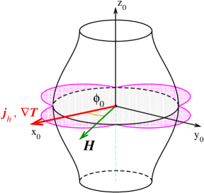
Figure 1: (Color online) The model considered in this paper. Calculation of the thermal conductivity is done for a quasi-cylindrical Fermi surface, when the heat current or temperature gradient and (rotated) magnetic field are in the $ab$-plane. The order parameter is assumed to have a $d$-wave symmetry.

In the following section we briefly review the approach and the main results of the preceding paper, such as the closed form expressions for the Green’s functions necessary for computing linear response to the gradient of temperature. Sec. III gives the derivation of the thermal conductivity using Keldysh formulation for the non-equilibrium theory of superconductivity, with some details relegated to Appendix A. As in I, we find that the simple example of a 2D $d$-wave superconductor with a cylindrical Fermi surface provides a semi-analytically accessible path towards understanding some of the crucial features of our results, and consider it in Sec. IV. Sec. V is devoted to the calculations for more realistic quasi-cylindrical Fermi surface (Fig. 1), and at the end of it we discuss the results, compare them with the data on CeCoIn₅ and organic $\kappa-(BEDT)-TTF$.

Our Secs. IV,  V, and  VI are intended for those readers who are interested only in the overall physical picture and the behavior of the measured properties; the figures in Sec. V show the main differences between the self-consistent and non-self-consistent calculations. Finally, our conclusions provide a side-by-side comparison of the specific heat discussed in I and the thermal conductivity results, and outline implications for future experiments.

II Quasiclassical Approach and the equilibrium Green’s function

II.1 Basic equations and formulation

We follow Ref. I in considering the quasiclassical (integrated over the quasiparticle band energy) Green’s function in a singlet superconductor in magnetic field Eilenberger (1968); Larkin and Ovchinnikov (1969); Serene and Rainer (1983); Alexander et al. (1985); Houghton and Vekhter (1998); Eschrig et al. (1999). In the spin and particle-hole (Nambu) space the matrix propagator depends on the direction at the Fermi surface (FS), $\hat{{\bf p}}$, and the center of mass coordinate, ${\bf R}$, and is

$$\widehat{g}({\bf R},\hat{{\bf p}};\varepsilon)=\left(\begin{array}[]{cc}g&i\sigma_{2}f\\ i\sigma_{2}\underline{f}&-g\end{array}\right)\,.$$ (1)

We write the quasiclassical equation for the real-energy, $\varepsilon$, retarded, advanced, and Keldysh propagators, which enables us to carry out non-equilibrium calculations, see Appendix A below and Refs. Serene and Rainer, 1983; Rainer and Sauls, 1995; Graf et al., 1996. The retarded (R) and advanced (A) functions $\widehat{g}=\widehat{g}^{R,A}$ satisfy (we take convention $e<0$)

$$[(\varepsilon+{e\over c}{\bf v}_{f}(\hat{{\bf p}}){\bf A}({\bf R}))\,\widehat{\tau}_{3}-\widehat{\Delta}({\bf R},\hat{{\bf p}})-\widehat{\sigma}_{imp}({\bf R};\varepsilon),$$

$$\widehat{g}({\bf R},\hat{{\bf p}};\varepsilon)]+i{\bf v}_{f}(\hat{{\bf p}})\cdot\mbox{\boldmath$\nabla_{\mbox{\tiny${\bf R}$}}$}\;\widehat{g}({\bf R},\hat{{\bf p}};\varepsilon)=0\,,$$ (2)

together with the normalization condition

$$\widehat{g}^{R,A}({\bf R},\hat{{\bf p}};\varepsilon_{m})^{2}=-\pi^{2}\widehat{1}\,.$$ (3)

Here ${\bf v}_{f}(\hat{{\bf p}})$ is the Fermi velocity at a point $\hat{{\bf p}}$ on the FS. The vector potential ${\bf A}({\bf R})$ describes the applied magnetic field, and the self-energy, $\widehat{\sigma}$, (different for the retarded and the advanced components) is due to impurity scattering. The mean field singlet order parameter,

$$\widehat{\Delta}=\left(\begin{array}[]{cc}0&i\sigma_{2}\Delta\\ i\sigma_{2}\Delta^{*}&0\end{array}\right)\,,$$ (4)

is self-consistently determined using the Keldysh functions $f^{K}$,

$$\Delta({\bf R},\hat{{\bf p}})=\int{d\varepsilon\over 4\pi i}\,\langle\,V(\hat{{\bf p}},\hat{{\bf p}}^{\prime})\,f^{K}({\bf R},\hat{{\bf p}}^{\prime};\varepsilon)\rangle_{\mbox{\tiny FS}}\,\,.$$ (5)

In Eq.(5) we used a shorthand notation

$$\langle\;\bullet\;\rangle_{\mbox{\tiny FS}}=\int d\hat{{\bf p}}_{\mbox{\tiny FS}}\;n_{f}(\hat{{\bf p}})\;\bullet\,,$$ (6)

where $n_{f}(\hat{{\bf p}})=N_{f}(\hat{{\bf p}})/{\cal N}_{f}$, with $N_{f}(\hat{{\bf p}})$ the density of states (DOS) at a point $\hat{{\bf p}}$ on the Fermi surface in the normal state, and ${\cal N}_{f}=\int d\hat{{\bf p}}_{\mbox{\tiny FS}}N_{f}(\hat{{\bf p}})$ the net density of states.

Throughout our work we use a separable pairing interactions,

$$V(\hat{{\bf p}},\hat{{\bf p}}^{\prime})=V_{s}\,{\cal Y}(\hat{{\bf p}})\,{\cal Y}(\hat{{\bf p}}^{\prime})\,,$$ (7)

where ${\cal Y}(\hat{{\bf p}})$ is the normalized basis function for the angular momentum representation, $\langle{\cal Y}(\hat{{\bf p}})^{2}\rangle_{{\mbox{\tiny FS}}}=1$. Hence the order parameter is $\Delta({\bf R},\hat{{\bf p}})=\Delta({\bf R}){\cal Y}(\hat{{\bf p}})$. For example, for a 2D $d_{x^{2}-y^{2}}$ gap we take ${\cal Y}(\hat{{\bf p}})=\sqrt{2}({\widehat{p}}_{x}^{2}-{\widehat{p}}_{y}^{2})$.

We include the impurity scattering via the self-consistent $t$-matrix approximation, with the self-energy

$$\widehat{\sigma}_{imp}({\bf R};\varepsilon)=\left(\begin{array}[]{cc}D+\Sigma&i\sigma_{2}\Delta_{imp}\\ i\sigma_{2}\underline{\Delta}_{imp}&D-\Sigma\end{array}\right)=n_{imp}\hat{t}({\bf R};\varepsilon)\,.$$ (8)

Here $n_{imp}$ is the impurity concentration, and, if $u$ is the isotropic single impurity potential, the $t$-matrix is defined via

$$\hat{t}({\bf R};\varepsilon)=u\hat{1}+u{\cal N}_{f}\langle\widehat{g}({\bf R},\hat{{\bf p}};\varepsilon)\rangle_{\mbox{\tiny FS}}\;\hat{t}({\bf R};\varepsilon)\,.$$ (9)

The component labeled $D\,\widehat{1}$ drops out of the equations for the retarded and the advanced Green’s functions since the unit matrix commutes with the Green’s function in Eq. (2). This term, however, appears in the Keldysh part, and affects the transport properties Hirschfeld et al. (1988); Löfwander and Fogelström (2004) (see also Appendix A). Below we parameterize the scattering by the “bare” scattering rate, $\Gamma=n_{imp}/\pi{\cal N}_{f}$, and the phase shift $\delta_{0}$ of the impurity scattering, $\tan\delta_{0}=\pi u{\cal N}_{f}$.

II.2 Equilibrium Green’s function

In I we solved the quasiclassical equations in the vortex state. We took the superconducting order parameter in the form $\Delta(\bm{R},\hat{{\bf p}})=\Delta(\bm{R}){\cal Y}(\hat{{\bf p}})$, where

$$\Delta(\bm{R})=\sum_{n}\Delta_{n}\mbox{$\displaystyle\langle\,{\bf R}\,|\,n\,\rangle$}$$ (10a)

$$\mbox{$\displaystyle\langle\,{\bf R}\,|\,n\,\rangle$}=\sum_{k_{y}}C_{k_{y}}^{(n)}{e^{ik_{y}\sqrt{S_{f}}y}\over\sqrt[4]{S_{f}\Lambda^{2}}}\widetilde{\Phi}_{n}\left(x,k_{y}\right)\,.$$ (10b)

We showed that for $\sum_{k_{y}}|C_{k_{y}}^{(n)}|^{2}=1$ the coefficients $C_{k_{y}}^{(n)}$ determine the shape of the lattice, while $\Delta_{n}$ is the amplitude of the order parameter in the $n$-th Landau level channel. The expansion of $\Delta(\bm{R})$ is in the Landau level function of the renormalized coordinates,

$$\widetilde{\Phi}_{n}(x,k_{y})=\Phi_{n}\left({x-\Lambda^{2}\sqrt{S_{f}}k_{y}\over\Lambda\sqrt{S_{f}}}\right)\,.$$ (11)

The anisotropy factor, $S_{f}$, for the field applied at an angle $\theta_{H}$ to the $z$-axis, is

$$S_{f}=\sqrt{\cos^{2}\theta_{H}+{v_{0||}^{2}\over v_{0\perp}^{2}}\sin^{2}\theta_{H}}\,,$$ (12)

where $v_{0\perp}^{2}=2\langle{\cal Y}^{2}(\hat{{\bf p}})v^{2}_{\perp i}(p_{z})\rangle_{\mbox{\tiny FS}}$ and $v_{0\parallel}^{2}=2\langle{\cal Y}^{2}(\hat{{\bf p}})v^{2}_{\parallel}(p_{z})\rangle_{\mbox{\tiny FS}}$; here $v_{\parallel}$ is the projection of the Fermi velocity on the $z$ axis, and $v_{\perp i}$ with $i=x,y$ is the projection on the axes in the plane normal to $z$.

Following the BPT procedure we replaced the diagonal part of the Green’s function, $g$, with its spatial average, and introduced the ladder operators for the Landau levels which allowed us to solve for the anomalous (Gorkov) functions in terms of $g$,

$$f({\bf R},\hat{{\bf p}};\varepsilon)=\sum_{m}f_{m}(\hat{{\bf p}},\varepsilon)\mbox{$\displaystyle\langle\,{\bf R}\,|\,m\,\rangle$}\,,$$ (13a)

$$f_{m}(\hat{{\bf p}},\varepsilon)=ig\,\sum_{n}(-\tilde{v}_{-}(\hat{{\bf p}}))^{m-n}\,{\cal D}_{m,n}(\varepsilon,|\hat{{\bf p}}|)\widetilde{\Delta}_{n}(\hat{{\bf p}};\varepsilon)\,.$$ (13b)

Here

$$\tilde{v}_{\pm}(\hat{{\bf p}})=\frac{\tilde{v}_{f}(\hat{{\bf p}})_{x}\pm i\tilde{v}_{f}(\hat{{\bf p}})_{y}}{|\tilde{v}_{f}^{\perp}|}\,,$$ (14)

with

$$\tilde{v}_{f}(\hat{{\bf p}})_{x}=v_{f}(\hat{{\bf p}})_{x}/\sqrt{S_{f}}\quad,\quad\tilde{v}_{f}(\hat{{\bf p}})_{y}=v_{f}(\hat{{\bf p}})_{y}\sqrt{S_{f}}\,,$$ (15)

and

$$|\tilde{v}_{f}^{\perp}(\hat{{\bf p}})|=\sqrt{\tilde{v}_{f}(\hat{{\bf p}})_{x}^{2}+\tilde{v}_{f}(\hat{{\bf p}})_{y}^{2}}\,$$ (16)

The coefficients of the expansion are given by

$${\cal D}_{m,n}(\varepsilon,|\hat{{\bf p}}|)=\sqrt{\pi}{2\Lambda\over|\tilde{v}^{\perp}_{f}|}\sum_{j=0}^{min(m,n)}(-1)^{n_{1}}D_{m,n}^{n_{1},n_{2}}\left({2\tilde{\varepsilon}\Lambda\over|\tilde{v}^{\perp}_{f}|}\right)\,,$$ (17)

with $n_{1}(j)=j+(|m-n|-(m-n))/2$, $n_{2}(j)=j+(|m-n|+(m-n))/2$ in each term and

$$D^{n_{1},n_{2}}_{m,n}(z)=\left({-i\over\sqrt{2}}\right)^{n_{1}+n_{2}}{\sqrt{n!}\sqrt{m!}\over(n-n_{1})!n_{1}!n_{2}!}W^{(n_{1}+n_{2})}(z)\,,$$ (18)

where $W^{(n)}(z)$ is the $n$-th derivative of the function $W(z)=\exp(-z^{2})\mbox{erfc}(-iz)$.

We then use the normalization condition,

$$g^{2}-\overline{\underline{f}\,f}=-\pi^{2}\,,$$ (19)

in the spatially averaged form, with $\overline{f_{1}\,f_{2}}$ the spatial average of the product, to find the equilibrium Green’s function

$$g = -i\pi/\sqrt{1+P}\,,$$ (20a)

$$P = -i\sqrt{\pi}{2\over w^{2}}\sum_{n}\sum_{m}\widetilde{\underline{\Delta}}_{n}\widetilde{\Delta}_{m}\sum^{\prime}_{k,l\geq 0}\frac{(\tilde{v}_{+})^{l}(-\tilde{v}_{-})^{k}}{l!\,k!}$$ (20b)

$$\times\mbox{$\displaystyle\langle\,n\,|$}a^{{\dagger}k}a^{l}\mbox{$\displaystyle|\,m\,\rangle$}\left({-i\over\sqrt{2}}\right)^{k+l}W^{(k+l+1)}\left({\sqrt{2}\tilde{\varepsilon}\over w}\right)\,,$$

where $w=|\tilde{v}^{\perp}_{f}|/\sqrt{2}\Lambda$, and the prime over the $k,l$-sum denotes the restriction that the matrix element $\mbox{$\displaystyle\langle\,n\,|$}a^{{\dagger}k}a^{l}\mbox{$\displaystyle|\,m\,\rangle$}=\sqrt{n!m!/(n-k)!(m-l)!}$ is non-zero only for $k\leq n$, $l\leq m$ and $k-l=n-m$. This expression reduces to the form of $g$ obtained previously if we truncate the order parameter expansion at the lowest Landau level Pesch (1975); Klimesch and Pesch (1978); Houghton and Vekhter (1998); Vekhter and Houghton (1999); Kusunose (2004).

$$g=\frac{-i\pi}{\sqrt{1-i\sqrt{\pi}\left(\frac{2\Lambda}{|\tilde{v}_{f}^{\perp}|}\right)^{2}\,W^{\prime}(\frac{2\tilde{\varepsilon}\Lambda}{|\tilde{v}_{f}^{\perp}|})\,\widetilde{\Delta}_{0}\underline{\widetilde{\Delta}}_{0}}}\,.$$ (21)

This latter form is useful for semi-analytical calculations.

III Heat conductivity

III.1 Linear response and thermal conductivity

We now proceed to derivation and analysis of expression for the thermal conductivity in the linear response theory. We first derive the general formula for the heat conductivity tensor, based on the closed-form solution for the quasiclassical retarded and advanced propagators found above, and using the non-equilibrium Keldysh approach. The Keldysh part of the full quasiclassical Green’s function carries information about both the spectrum and the distribution of quasiparticles, and the heat current is defined as energy transfer by quasiparticlesSerene and Rainer (1983); Graf et al. (1996)

$${\bf j}_{h}({\bf R})=2N_{f}\int d\hat{{\bf p}}\;n_{f}(\hat{{\bf p}}){\bf v}_{f}(\hat{{\bf p}})\int\limits_{-\infty}^{+\infty}{d\varepsilon\over 4\pi i}\varepsilon g^{K}(\hat{{\bf p}},{\bf R};\varepsilon)\,,$$ (22)

where $g^{K}$ is the diagonal component of the Keldysh propagator.

In equilibrium ${\bf j}_{h}=0$ as expected, and in linear response we define the heat conductivity tensor $\hat{\kappa}$ via ${\bf j}_{h}=-\hat{\kappa}\mbox{\boldmath$\nabla$}T$. We linearize the equations to find the first order corrections to the retarded, advanced and Keldysh propagators, $\delta\widehat{g}^{R,A,K}$, with respect to $\mbox{\boldmath$\nabla$}T$. This implicitly assumes that the inhomogeneity due to the temperature gradient is much smaller and occurs on much longer scales than the inhomogeneity due to vortices, impurities, etc., which is the case experimentally. The details of the derivation of $\kappa$ are presented in Appendix A and here we give only the final expression,

$${\kappa_{ij}\over T}=\frac{N_{f}}{2}\int{d\varepsilon\over T}\frac{\varepsilon^{2}}{T^{2}\cosh^{2}(\varepsilon/2T)}\int d{\bf p}_{\mbox{\tiny FS}}\,n_{f}(\hat{{\bf p}})\;v_{f,i}(\hat{{\bf p}})v_{f,j}(\hat{{\bf p}})\;\frac{-iG_{2}}{G_{1}G_{4}-G_{2}G_{3}}(-{1\over\pi}\mathfrak{Im}\,g^{R})$$ (23a)

where we defined,

$$G_{1} = -D^{a}+\frac{1}{2(g^{R}-g^{A})}\,\overline{[-(f^{R}+f^{A})(\underline{\widetilde{\Delta}}^{R}-\underline{\widetilde{\Delta}}^{A})+(\underline{f}^{R}+\underline{f}^{A})(\widetilde{\Delta}^{R}-\widetilde{\Delta}^{A})]}$$ (23b)

$$G_{2} = -\Sigma^{a}+\frac{1}{2(g^{R}-g^{A})}\,\overline{[(f^{R}-f^{A})(\underline{\widetilde{\Delta}}^{R}-\underline{\widetilde{\Delta}}^{A})+(\underline{f}^{R}-\underline{f}^{A})(\widetilde{\Delta}^{R}-\widetilde{\Delta}^{A})]}$$ (23c)

$$G_{3} = -\Sigma^{a}+\frac{1}{2(g^{R}-g^{A})}\,\overline{[(f^{R}+f^{A})(\underline{\widetilde{\Delta}}^{R}+\underline{\widetilde{\Delta}}^{A})+(\underline{f}^{R}+\underline{f}^{A})(\widetilde{\Delta}^{R}+\widetilde{\Delta}^{A})]}$$ (23d)

$$G_{4} = -D^{a}+\frac{1}{2(g^{R}-g^{A})}\,\overline{[-(f^{R}-f^{A})(\underline{\widetilde{\Delta}}^{R}+\underline{\widetilde{\Delta}}^{A})+(\underline{f}^{R}-\underline{f}^{A})(\widetilde{\Delta}^{R}+\widetilde{\Delta}^{A})]}\,,$$ (23e)

and used the following notations: $D^{a}(\varepsilon)=D^{R}(\varepsilon)-D^{A}(\varepsilon)$, $\Sigma^{a}(\varepsilon)=\Sigma^{R}(\varepsilon)-\Sigma^{A}(\varepsilon)$, and $\widetilde{\Delta}^{R,A}({\bf R},\hat{{\bf p}};\varepsilon)=\Delta({\bf R},\hat{{\bf p}})+\Delta^{R,A}_{imp}({\bf R};\varepsilon)$. In both Born and unitarity scattering limits $D^{a}=0$, which simplifies this resultHirschfeld et al. (1988); Graf et al. (1996).

We can re-write Eq. (23a) as

$$\frac{\kappa_{ij}(T,H)}{T}=\int\limits^{+\infty}_{-\infty}\;\frac{d\varepsilon}{2T}\frac{\varepsilon^{2}}{T^{2}}\cosh^{-2}\frac{\varepsilon}{2T}$$ (24)

$$\times\int\,d{\bf p}_{\mbox{\tiny FS}}\,v_{f,i}v_{f,j}\,N(T,\bm{H};\hat{{\bf p}},\varepsilon)\;\tau_{H}(T,H;\hat{{\bf p}},\varepsilon)\,.$$

Here $N(T,H;\hat{{\bf p}},\varepsilon)=N_{f}n_{f}(\hat{{\bf p}})(-\mathfrak{Im}\,\,g^{R}/\pi)$ is the angle-dependent DOS, and $\tau_{H}=-iG_{2}/(G_{1}G_{4}-G_{2}G_{3})$ has the meaning of the transport lifetime due to both impurity and vortex scattering. In the normal state $\tau_{H}=\tau_{n}=1/2\gamma$ ($\gamma=\Gamma\sin^{2}\delta_{0}$) and $-\mathfrak{Im}\,\,g^{R}/\pi=1$. Notice that the transport and the single-particle lifetimes are different.

Several limiting cases are useful for developing a qualitative understanding of the physical picture. In the Born or unitary limit $D^{R}=D^{A}=0$. If we truncate the expansion of the vortex state at the lowest Landau level function, $n=0$, and neglect the off-diagonal impurity self-energy $\Delta_{imp}=0$, we obtain from Eqs.(13b-20)

$$g^{R} = \frac{-i\pi}{\sqrt{1-i\sqrt{\pi}\left(\frac{2\Lambda}{|\tilde{v}_{f}^{\perp}|}\right)^{2}\,W^{\prime}(\frac{2\tilde{\varepsilon}\Lambda}{|\tilde{v}_{f}^{\perp}|})\,|\Delta_{0}{\cal Y}(\hat{\bf p})|^{2}}}\,$$ (25)

$$\overline{\underline{\Delta}f^{R}} = ig^{R}\;\frac{2\sqrt{\pi}\Lambda}{|\tilde{v}_{f}^{\perp}|}W\left(\frac{2\tilde{\varepsilon}\Lambda}{|\tilde{v}_{f}^{\perp}|}\right)\;|\Delta_{0}{\cal Y}(\hat{\bf p})|^{2}\,.$$ (26)

In this approximation $\widetilde{\Delta}^{R}=\widetilde{\Delta}^{A}=\Delta$ and thus $G_{1}=0$, so for the thermal transport lifetime we find,

$$\frac{1}{2\tau_{H}}=-\mathfrak{Im}\,\Sigma^{R}+\sqrt{\pi}{2\Lambda\over|\tilde{v}_{f}^{\perp}|}\frac{\mathfrak{Im}\,[g^{R}\,W(2\tilde{\varepsilon}\Lambda/|\tilde{v}_{f}^{\perp}|)]}{\mathfrak{Im}\,\,g^{R}}|\Delta_{0}{\cal Y}|^{2}\,.$$ (27)

which agrees with results in Ref. Vekhter and Houghton, 1999. We, however, aim to include the higher components of the order parameter expansion for a fully self-consistent calculation and for comparison with experiment.

III.2 General properties of the thermal conductivity tensor

As in I we focus on a tetragonal system with an open, along the $z$-axis, Fermi surface, and the magnetic field applied in the $xy$ plane, at angle $\phi_{0}$ to the $x$-axis. We consider both $d_{x^{2}-y^{2}}$ and $d_{xy}$ order parameters, and model their variation around the Fermi surface by ${\cal Y}(\phi)=\sqrt{2}\cos 2\phi$ and ${\cal Y}(\phi)=\sqrt{2}\sin 2\phi$ respectively, where $\phi$ is the angle between the projection of the Fermi momentum on the basal plane and the $x$ axis. As before, we will consider both a cylindrical (no energy dispersion along $z$), and quasi-cylindrical (tight-binding dispersion along $z$) Fermi surfaces. The following considerations are valid irrespective of the Fermi surface shape.

Experimentally, the in-plane (interplane) heat conductivity is measured by driving the heat current along a high symmetry crystalline direction, such as [100] or [110] ([001]). The longitudinal and/or transverse thermal gradient are defined and measured with respect to the direction of the heat current. This creates two physically distinct cases for the in-plane transport: the heat flow in the experiment is along either a node or antinode, see Fig. 2. If our task is, for example, to determine the shape of the gap from the measured thermal conductivity along the $x$-axis we cannot a priori assume whether the heat current is along a node or a gap maximum.

From the theoretical perspective, the knowledge of the full thermal conductivity tensor, Eq. (23a) allows to determine the heat transport along an arbitrary direction. The two cases, $d_{x^{2}-y^{2}}$ and $d_{xy}$, see Fig. 2, transform into one another by rotation of the heat current: thermal conductivity measured for the heat current in the [100] direction for the $d_{xy}$ gap is equal to the thermal conductivity for the $d_{x^{2}-y^{2}}$ order parameter with the heat current in [110] direction. Therefore we focus on the $d_{x^{2}-y^{2}}$, and compute all the components $\kappa_{ij}$ in the plane; the thermal conductivity for the $d_{xy}$ case is computed using these results. In a tetragonal system in the absence of the field, the off-diagonal elements $\kappa_{xy}=\kappa_{yx}=0$, and the diagonal elements are equal, $\kappa_{xx}=\kappa_{yy}$, so that the conductivity is isotropic. Applying a magnetic field in the plane changes the situation dramatically. First, for the field applied at an angle $\phi_{0}$ relative to the [100] direction, $\kappa_{xx}\neq\kappa_{yy}$; it is easy to see (and we show it formally below) that $\kappa_{yy}(\phi_{0})=\kappa_{xx}(\pi/2+\phi_{0})$ since for these components the angle between the field and the heat current is the same.

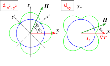
Figure 2: (Color online) Two distinct experimentally relevant setups for the thermal conductivity. Left panel: $d_{x^{2}-y^{2}}$ gap symmetry, right panel: $d_{xy}$ gap symmetry. Response of the $d_{xy}$ superconductor to the thermal gradient along the [100] (${\bf x}$) direction with the field at an angle $\phi_{0}^{\prime}$ to this axis is equivalent to the response of a $d_{x^{2}-y^{2}}$ system to the thermal gradient along the [110] (${\bf x}^{\prime}$) direction and the field at the angle $\phi_{0}=\phi^{\prime}+\pi/4$ to the ${\bf x}$-axis. Note that the expriment is done with the heat current ${\bf j}_{h}$ along [100], while the calculations are for the thermal gradient along this direction, see text for details.

Second, the in-plane field breaks the tetragonal symmetry, and therefore $\kappa_{xy}(\phi_{0})\neq 0$ for a general orientation of the field. We emphasize that this occurs even when the Lorenz force is neglected. The non-vanishing $\kappa_{xy}$ arises because of the difference between the transport along the vortex and normal to it; when the field (and the vortices) are at an arbitrary angle to the direction of the heat current, a transverse temperature gradient appears similar to the Hall conductivity in a material with the electric field applied at an arbitrary angle to inequivalent principal axes. The transverse heat conductivity is of the same order or magnitude as the anisotropy between transport parallel and normal to the vortices, and hence much greater than the typical contribution proportional to the cyclotron frequency, $\omega_{c}=eH/mc\sim(\Delta^{2}/E_{f})(H/H_{c2})$. Therefore the Hall angle is moderately large, see below.

To make the argument more rigorous consider the general form of the heat conductivity tensor as a function of the field orientation, $\hat{{\bf H}}$. We write Eq. (23a) in the form,

$$\kappa_{ij}(\phi_{0})=\langle v_{f,i}(\hat{{\bf p}})v_{f,j}(\hat{{\bf p}})\;{\cal K}((\hat{{\bf p}}_{f}\cdot\hat{{\bf H}})^{2},|\Delta(\hat{{\bf p}})|^{2};T,H)\rangle\,.$$ (28)

Here the kernel ${\cal K}((\hat{{\bf p}}_{f}\cdot\hat{{\bf H}})^{2},|\Delta(\hat{{\bf p}})|;T,H)$ is determined by the equilibrium Green’s functions, and, at a given point ${\widehat{{\bf p}}}_{f}$ at the Fermi surface, depends on the angle between the Fermi velocity and the field, $(\hat{{\bf p}}_{f}\cdot\hat{{\bf H}})$, the gap amplitude for that direction, $|\Delta(\hat{{\bf p}})|$, as well as on $T$ and $H$. Since the kernel does not change if the direction of the field is reversed, we explicitly write it as dependent on $(\hat{{\bf p}}_{f}\cdot\hat{{\bf H}})^{2}$

Let us start by considering a $d_{x^{2}-y^{2}}$ gap. The inversion of the field in the $xy$-plane corresponds to the change $\phi_{0}\to\phi_{0}+\pi$. We can simultaneously change the variables in Eq. (28) according to $(\hat{p}_{x},\hat{p}_{y})\to(-\hat{p}_{x},-\hat{p}_{y})$, which leaves the kernel invariant, and find

$$\kappa_{ij}(\phi_{0}+\pi)=\kappa_{ij}(\phi_{0})\,,$$ (29)

for $i,j=\{x,y\}$; at the same time $\kappa_{iz}(\phi_{0}+\pi)=-\kappa_{iz}(\phi_{0})$, and $\kappa_{zz}(\phi_{0}+\pi)=\kappa_{zz}(\phi_{0})$. Similarly, reflection of the field in the $xz$-plane, $\phi_{0}\to-\phi_{0}$, together with reflection $\hat{p}_{y}\to-\hat{p}_{y}$ again does not change the kernel, and leads to

$$\kappa_{xx}(-\phi_{0}) = \kappa_{xx}(\phi_{0})\,,$$

$$\kappa_{yy}(-\phi_{0}) = \kappa_{yy}(\phi_{0})\,,$$ (30)

$$\kappa_{xy}(-\phi_{0}) = -\kappa_{xy}(\phi_{0})\,.$$

Finally, if we rotate the field and the coordinate system, $\phi_{0}\to\phi_{0}+\pi/2$ [$(\hat{p}_{x},\hat{p}_{y})\to(\hat{p}_{y},-\hat{p}_{x})$], we find

$$\kappa_{xx}(\phi_{0}+\pi/2) = \kappa_{yy}(\phi_{0})\,,$$

$$\kappa_{yy}(\phi_{0}+\pi/2) = \kappa_{xx}(\phi_{0})\,,$$ (31)

$$\kappa_{xy}(\phi_{0}+\pi/2) = -\kappa_{xy}(\phi_{0})\,.$$

We carry out Fourier expansion based on these symmetries. From Eq. (29), Eq. (30), and Eq. (31) we find for the $d_{x^{2}-y^{2}}$ gap

$$\kappa_{xx}(\phi_{0}) = \kappa_{0}+\kappa_{2}\cos 2\phi_{0}+\kappa_{4}\cos 4\phi_{0}+\dots\,,$$

$$\kappa_{yy}(\phi_{0}) = \kappa_{0}-{\kappa}_{2}\cos 2\phi_{0}+{\kappa}_{4}\cos 4\phi_{0}+\dots\,,$$ (32)

$$\kappa_{xy}(\phi_{0}) = \tilde{\kappa}_{2}\sin 2\phi_{0}+\tilde{\kappa}_{6}\sin 6\phi_{0}+\dots\,.$$

The $\cos 2\phi_{0}$ term in the longitudinal conductivity describes the anisotropy between the transport along and normal to the vortices. Furthermore, if the superconducting gap is isotropic (or absent), and hence the only dependence of the kernel $K$ on the field orientation is via the term $(\hat{{\bf p}}_{f}\cdot\hat{{\bf H}})^{2}$, it immediately follows that for our cylindrically symmetric Fermi surface $\kappa_{xx}+\kappa_{yy}$ is independent of the field orientation, $\phi_{0}$, which requires $\kappa_{4}=0$. For an anisotropic Fermi surface there may be an angular modulation of the thermal conductivity, but it would occur already in the normal state. Therefore the $\cos 4\phi_{0}$ component that appears only in the superconducting state is predominantly due to the gap anisotropy. Such a decomposition in the analysis of the experimentally measured thermal conductivity was used in Refs. Izawa et al., 2001, 2002a; Matsuda et al., 2006 to infer the gap structure of heavy fermion and organic quasi-two-dimensional materials; and in the following section we compare our results with their analysis.

The origin of the $\sin 2\phi_{0}$ directional dependence of the transverse thermal conductivity is also transparent. In the presence of the field, the principal axes of the thermal conductivity tensor are along and normal to ${\bf H}$. Consequently, when the heat current is along one of those axes, no transverse signal is generated, irrespective of the nodal structure. This is precisely the result found in high-T_c superconductors by Ocaña and Esquinazi Ocaña and Esquinazi (2001, 2002), who observed a nearly perfect sinusoidal thermal Hall response.

We are now in the position to consider the differences between the $d_{x^{2}-y^{2}}$ and $d_{xy}$ gaps. The longitudinal and transverse conductivities for the $d_{xy}$ order parameter are identical to the components of the thermal conductivity tensor for the $d_{x^{2}-y^{2}}$ case in the coordinates $(x^{\prime},y^{\prime})$ rotated by $\alpha=\pi/4$ with respect to $(x,y)$, see Fig. 2,

$$\hat{\kappa}^{\prime}=\hat{\kappa}_{d_{xy}}=\left(\begin{array}[]{cc}\kappa_{x^{\prime}x^{\prime}}&\kappa_{x^{\prime}y^{\prime}}\\ \kappa_{x^{\prime}y^{\prime}}&\kappa_{y^{\prime}y^{\prime}}\end{array}\right)\,.$$ (33)

Moreover, the field applied at an angle $\phi_{0}^{\prime}$ to the ${\bf x}^{\prime}$ axis makes angle $\phi_{0}=\phi^{\prime}+\pi/4$ with the ${\bf x}$ axis, so that $\hat{\kappa}^{\prime}(\phi_{0}^{\prime})=\hat{{\cal R}}(\alpha)\hat{\kappa}(\phi_{0}^{\prime}+\pi/4)\hat{{\cal R}}^{-1}(\alpha)$, with the rotation matrix

$$\hat{{\cal R}}=\left(\begin{array}[]{cc}\cos\alpha&\sin\alpha\\ -\sin\alpha&\cos\alpha\end{array}\right)\,.$$ (34)

This leads to

$$\kappa_{x^{\prime}x^{\prime}}(\phi_{0}^{\prime}) = \kappa_{0}+\tilde{\kappa}_{2}\cos 2\phi_{0}^{\prime}-\kappa_{4}\cos 4\phi_{0}^{\prime}+\dots\,,$$

$$\kappa_{y^{\prime}y^{\prime}}(\phi_{0}^{\prime}) = \kappa_{0}-\tilde{\kappa}_{2}\cos 2\phi_{0}^{\prime}-\kappa_{4}\cos 4\phi_{0}^{\prime}+\dots\,,$$ (35)

$$\kappa_{x^{\prime}y^{\prime}}(\phi_{0}^{\prime}) = -{\kappa}_{2}\sin 2\phi_{0}^{\prime}+\dots\,.$$

Importantly, this result implies that the four-fold term in the longitudinal thermal conductivity depends only on the orientation of the field with respect to the nodes of the gap. Indeed, let us restore the dependence on the angle $\phi_{0}$ measured to the gap maximum, then

$$\kappa_{x^{\prime}x^{\prime}}(\phi_{0}) = \kappa_{0}+\tilde{\kappa}_{2}\sin 2\phi_{0}+\kappa_{4}\cos 4\phi_{0}+\dots\,,$$ (36)

$$\kappa_{x^{\prime}y^{\prime}}(\phi_{0}) = {\kappa}_{2}\cos 2\phi_{0}+\dots\,.$$ (37)

The last term in the longitudinal thermal conductivity for the $d_{xy}$ order is identical to that for the $d_{x^{2}-y^{2}}$ gap. In other words, independently of the gap symmetry, the fourfold term in the longitudinal thermal conductivity simply depends on the angle between the direction of the in-plane field, and the antinodal direction of the gap. Consequently, in the following sections we will focus both on the overall features of the thermal transport and specifically on that term.

III.3 Calculated vs. measured thermal conductivity

We will see below that the field-induced anisotropy in the transport along and normal to the vortices leads to the large thermal Hall angle, $\kappa_{xy}/\kappa_{xx}\sim 0.1$. In this case it is important to keep in mind that theoretical calculations are done under assumptions different from the typical steady-state experimental setup. The thermal conductivity tensor is defined via ${\bf j}_{h,i}=-\kappa_{ij}\mbox{\boldmath$\nabla$}_{j}T$, where ${\bf j}_{h}$ is the heat current. The experiments are done by driving the thermal current along a given ([100]) axis, while thermally insulating the sample in the transverse direction. The experiment measures the thermal gradients established under the conditions ${\bf j}_{h,x}=j_{h}$ and ${\bf j}_{h,y}=0$. Consequently, the measured longitudinal, $\kappa_{l}$ and the transverse, $\kappa_{t}$, thermal conductivities are

$$\kappa_{l} = \kappa_{xx}-\frac{\kappa_{xy}^{2}}{\kappa_{yy}}\,,$$ (38)

$$\kappa_{t} = \frac{{\bm{\nabla}}_{y}T}{{\bm{\nabla}}_{x}T}\kappa_{l}\approx\kappa_{xy}\frac{\kappa_{xx}}{\kappa_{yy}}\,.$$ (39)

Presence of the off-diagonal terms does not substantially modify the absolute value of the longitudinal or transverse conductivity since $\kappa_{xy}^{2}/(\kappa_{yy}\kappa_{xx})\sim 0.01$ at most, and therefore $\kappa_{l}\approx\kappa_{xx}$ and $\kappa_{t}\approx\kappa_{xy}$.

Note, however, that our principal interest is in the fourfold nodal term, $\kappa_{4}$, which is itself only a fraction of the longitudinal thermal conductivity. Assuming $\kappa_{0}\gg\kappa_{2},\kappa_{4}$ we find

$$\kappa_{l}^{(4)}\approx\kappa_{4}+\frac{\tilde{\kappa}_{2}^{2}}{2\kappa_{0}}.$$ (40)

In some region of the phase diagram, where $\kappa_{2}\gg\kappa_{4}$, the two terms may be comparable. Our results indicate this range to be rather small. We find that the magnitude of the fourfold term is slightly changed by accounting for the difference between the computed and the measured quantity; however, the main features remain unmodified. Hence in the following we discuss the overall features of the thermal conductivity profiles, and only briefly return to the difference between the computed and measured anisotropy in the conclusions.

IV Cylindrical Fermi surface

Once again we begin by considering the anisotropy of the longitudinal heat conductivity, $\kappa_{xx}(\phi_{0})$, for a cylindrical Fermi surface, ${\bm{v}}_{f}=(v_{f}\cos\phi,v_{f}\sin\phi,0)$ for $0\leq\phi\leq 2\pi$ and $-\pi/c\leq k_{z}\leq\pi/c$, where $c$ is the $c$-axis lattice spacing. As described in Ref. I, this FS does not allow for the self-consistent calculation of the order parameter in the vortex state for the in-plane field. As before, we restrict ourselves to the lowest order Landau wave function for the order parameter, take $\Delta(T,H)=\Delta(T,0)[1-H/H_{c2}]^{1/2}$, and use the corresponding results for the thermal conductivity, Eqns.(25),(26), and (27). We choose $H_{c2}^{ab}$ to be direction independent, and carry out the self-consistent calculation in temperature and impurity scattering according to Eqs.(25) and (27). The impurity self energy is determined in the unitarity limit with the normal state mean free path $\ell_{n}/\xi_{0}=70$, where $\xi_{0}$ is the coherence length. This toy model lends itself easily to numerical and, in some limits, semi-analytical work, and therefore allows investigation of the salient features of the behavior of $\kappa_{xx}$. We show below that this model gives qualitatively correct results for quasi-two dimensional systems. In the self-consistent calculation there is a node-antinode anisotropy in the upper critical field at low $T$, and the comparison (given below) between the cylindrical and corrugated Fermi surfaces elucidates the role of this anisotropy for the behavior of the thermal conductivity.

In general, to determine $\kappa_{xx}$ we need to self-consistently determine the DOS and the single particle lifetime as in the calculation of the specific heat, and then determine the transport time and the thermal conductivity. For the lowest Landau approximation these are given by Eqs. (25-27). At finite energies this procedure can only be carried out numerically, as shown below. First we make some analytical estimates at low temperatures, $T=0$, and therefore set $\varepsilon=0$. We consider a $d_{x^{2}-y^{2}}$ gap and focus on three values of the thermal conductivity: along the field, $\kappa_{xx}(\phi_{0}=0^{\circ})$, normal to the field, $\kappa_{xx}(\phi_{0}=90^{\circ})$, and for the field along the node, $\kappa_{xx}(\phi_{0}=45^{\circ})$.

Define the mean free path $\ell=v_{f}\tau_{0}$, where $(2\tau_{0})^{-1}=-\mathfrak{Im}\,\Sigma^{R}(\varepsilon=0)$ is the single particle lifetime, which depends on the net density of states, and hence is sensitive to the direction of the field, $\phi_{0}$, via the self-consistent $T$-matrix equation. The argument of the $W$-function and its derivatives in Eqs. (25-27) is then $z=i\Lambda/\ell_{\perp}$, where $\ell_{\perp}=\ell|\sin(\phi-\phi_{0})|$, and depends on the position, $\phi$, on the Fermi surface. Since we work in the regime $\ell=v_{f}\tau_{0}\gg\Lambda$, we can set $z=0$ for most values of $\phi$, except for the directions nearly parallel to the field, $|\phi-\phi_{0}|\leq\Lambda/\ell$ and $|\phi-\phi_{0}-\pi|\leq\Lambda/\ell$. Let us denote the contribution from this narrow range as $\kappa_{1}$, and the contribution from the angles outside of this range as $\kappa_{2}$, so that $\kappa_{xx}=\kappa_{1}+\kappa_{2}$.

We now estimate each contribution. For $|\phi-\phi_{0}|\leq\Lambda/\ell$ we use the expansion for large argument, $W(z)\approx i/(\sqrt{\pi}z)$ and $W^{\prime}(z)\approx-i/(\sqrt{\pi}z^{2})$ to estimate the contribution to the thermal conductivity as

$$\frac{\kappa_{1}(\phi_{0})}{TN_{f}\,v_{f}^{2}} \approx \frac{4\pi^{2}}{3}\tau_{0}(\phi_{0})\int_{\phi_{0}-\Lambda/\ell}^{\phi_{0}+\Lambda/\ell}\frac{\cos^{2}\phi\,d\phi}{[1+(\Delta\tau_{0})^{2}]^{3/2}}$$ (41)

$$\simeq \frac{4\pi^{2}}{3}\tau_{0}(\phi_{0})\frac{a_{1}(\phi_{0})}{[1+(\Delta\tau_{0})^{2}]^{3/2}},$$ (42)

where $a_{1}(0^{\circ})=2\Lambda/\ell$, $a_{1}(45^{\circ})=\Lambda/\ell$, and $a_{1}(90^{\circ})=2\Lambda^{3}/3\ell^{3}$.

Over the remainder of the Fermi surface we set $z=0$ and use $W(0)=1,W^{\prime}(0)=2i/\sqrt{\pi}$ to find for $T\rightarrow 0$

$$\frac{\kappa_{2}(\phi_{0})}{TN_{f}\,v_{f}^{2}} = \frac{2\pi^{2}}{3}\tau_{0}(\phi_{0})$$

$$\times \int^{\prime}\frac{d\phi}{2\pi}\,\frac{\cos^{2}\phi}{\sqrt{1+\delta^{2}\frac{\cos^{2}2\phi}{\sin^{2}(\phi-\phi_{0})}}}\frac{1}{1+\mu\frac{\cos^{2}2\phi}{|\sin(\phi-\phi_{0})|}}\,,$$

$$\delta^{2} = 8(\Lambda\Delta/v_{f})^{2}\,,$$ (44)

$$\mu = \frac{4\sqrt{\pi}\Lambda\Delta^{2}\tau}{v_{f}}=\frac{\sqrt{\pi}}{2}\frac{\ell}{\Lambda}\delta^{2}\,.$$ (45)

Here the prime denotes that we are integrating over the entire Fermi surface excluding the regions close to the field direction considered above. Notice that $\mu\gg\delta^{2}$, and therefore the behavior of the thermal conductivity is controlled to much greater extent by the transport lifetime than by the density of states. The transport lifetime is peaked along the nodal directions.

These observations enable some analytical progress starting from the high fields, $H\lesssim H_{c2}$. In that case $\delta^{2}\ll\mu\ll 1$, and we approximate the density of states by its normal state value, $N_{f}$. Consequently, $\tau_{0}=\tau_{n}$, where $\tau_{n}$ is the normal state scattering rate which has no dependence on the direction of the magnetic field. Defining $\kappa_{n}=\pi^{2}N_{f}v_{f}^{2}\tau_{n}T/3$ we find angular variation of the thermal conductivity is approximately given by

$$\frac{\kappa_{xx}(\phi_{0})}{\kappa_{n}}=\int^{\prime}\frac{d\phi}{2\pi}\,\frac{2\cos^{2}\phi}{1+\mu\frac{\cos^{2}2\phi}{|\sin(\phi-\phi_{0})|}}\,,$$ (46)

We assume here that $\mu\gg\Lambda/\ell$, which is satisfied nearly everywhere up to $H_{c2}$ for clean systems. Now consider the behavior of the thermal conductivity for different directions of the field just below the upper critical field. For small $\mu$ we find the conductivity along the field, $\kappa_{xx}(0^{\circ})\approx\kappa_{n}[1+(4/\pi)\mu\ln\mu]$, while the conductivity normal to the field is $\kappa_{xx}(90^{\circ})\approx\kappa_{n}(1-28\mu/15\pi)$. Finally, for the field along a node, $\kappa_{xx}(45^{\circ})\approx\kappa_{n}(1-16\mu/3\pi)$. Therefore in the immediate vicinity of the transition at low temperature we expect $\kappa_{xx}(90^{\circ})>\kappa_{xx}(45^{\circ})>\kappa_{xx}(0^{\circ})$, or nearly twofold profile of the thermal conductivity.

At lower fields and $T=0$ we enter the regime $\delta^{2}\lesssim 1\ll\mu$, where we can still approximate the density of states by the normal state value, but the thermal transport is restricted by sharp peaks in the lifetime for nodal quasiparticles, see Eq. (46). Linearizing the gap around the nodal points and carrying out the integration, we find $\kappa_{xx}(0^{\circ})\approx\kappa_{xx}(90^{\circ})\simeq\kappa_{n}/(2^{1/4}\mu^{1/2})$, and $\kappa_{xx}(45^{\circ})\approx\kappa_{n}/(2\mu^{1/2})$. Consequently in this regime we find $\kappa_{xx}(90^{\circ})\geq\kappa_{xx}(0^{\circ})>\kappa_{xx}(45^{\circ})$, suggesting a weak minimum for the field along the node. Remarkably, at low $T$ the conductivity normal to the vortex is always higher than that parallel to the field, but the amplitude of this anisotropy, and the relative position of the value of the thermal conductivity for the field applied along a node both change between $\mu\ll 1$ and $\mu\gg 1$.

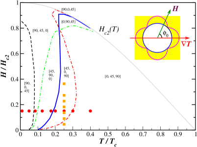
Figure 3: (Color online) Left panel: the $TH$-diagram of the longitudinal heat conductivity anisotropy, $\kappa_{xx}(\phi_{0})$. The thermal gradient is along the $x$-axis (maximal gap). Regions of different anisotropy are marked as $[\phi_{0}^{a},\phi_{0}^{b},\phi_{0}^{c}]$, which denotes $\kappa_{xx}(\phi_{0}^{a})>\kappa_{xx}(\phi_{0}^{b})>\kappa_{xx}(\phi_{0}^{c})$. For points marked by circles and squares the profiles of the angle-dependent $\kappa_{xx}(\phi_{0})$ are shown in Fig. 4.

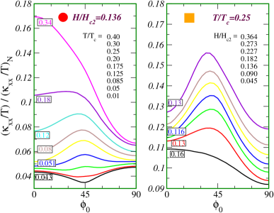
Figure 4: (Color online) Center panel: evolution of the heat conductivity with temperature for $H/H_{c2}\approx 0.14$. Right panel: heat conductivity as a function of the field angle for different fields at $T/T_{c}=0.25$. The curves are shifted vertically for clarity. The framed numbers give true values of normalized $\kappa_{xx}(\phi_{0}=0)$ for several of them. Corresponding temperatures and fields are shown in each panel in the same order as the curves.

This analysis is supported by the numerical results. We show results only for the longitudinal thermal conductivity, $d_{x^{2}-y^{2}}$ gap, and the heat current along the antinodal direction. The complete heat conductivity tensor is given and discussed below for the corrugated Fermi surface, with self-consistent calculations; The results for both FS are very similar.

The phase diagram of Fig. 3 shows regions with different anisotropy of the heat conductivity. The changes along the vertical axis, $T=0$, as a function of the field are in agreement with our estimates above: at $H\geq 0.85H_{c2}$ we find $\kappa_{xx}(90^{\circ})>\kappa_{xx}(45^{\circ})>\kappa_{xx}(0^{\circ})$, while below that field $\kappa_{xx}(90^{\circ})>\kappa_{xx}(0^{\circ})>\kappa_{xx}(45^{\circ})$. Note that for $H/H_{c2}=0.85$ we have $\delta^{2}\sim 1$ and therefore already $\mu\gg 1$. The variation of the thermal conductivity with the the direction of the applied field with respect to the x-axis (angle $\phi_{0}$) are shown in Fig. 4 for the points in the $T$-$H$ plane marked by circles and squares in Fig. 3. Evolution of $\kappa_{xx}$ with temperature at low fields (circles) is considerable: minimum for the nodal direction, $\phi_{0}=45^{\circ}$, at low $T$ quickly evolves into a maximum, and at $T/T_{c}\gtrsim 0.4$ the conductivity is largely twofold with no clear signature of the nodal structure of the gap. The change of the anisotropy with the field at moderate $T$ is more gradual (squares), and a pronounced peak at $\phi_{0}=45^{\circ}$, for the field along the nodes, persists to moderately high fields, providing a clear signature of the nodal structure.

The anisotropy between thermal transport normal to and parallel to the vortices is reversed at moderate temperatures (solid blue line in Fig. 3): at low temperature $\kappa_{xx}(0)<\kappa_{xx}(90)$ (in the notation of Eq. (32) this means $\kappa_{2}<0$), while at high $T$ we find $\kappa_{xx}(0)>\kappa_{xx}(90)$ (or $\kappa_{2}>0$). This evolution is in agreement with that for a conventional superconductor, found by Maki Maki (1967). Note also that the four-fold term $\sim\kappa_{4}$ in Eq. (32) is most pronounced at intermediate to low $T$ and $H$.

V Quasi-cylindrical Fermi surface

V.1 Main results

To solve the quasiclassical equations self-consistently for the order parameter, we need a model which allows for the $c$-axis superconducting currents when the field is applied in the $a$-$b$ plane. Hence we analyze a corrugated quasi-2D Fermi surface given by

$$p_{f}^{2}=p_{x}^{2}+p_{y}^{2}-(r^{2}\,p_{f}^{2})\cos(2s\,p_{z}/r^{2}p_{f})\,,$$

so that the quasiparticle velocity has a nonvanishing $z$-component, This Fermi surface, with $s=r=0.5$, was considered in I for the analysis of the specific heat, and we take the same values of parameters to directly compare the anisotropy of the heat capacity with that of thermal conductivity. Note that for this choice the DOS anisotropy in the normal state is $n_{f}(\hat{{\bf p}})=1$, and the normal state conductivity anisotropy is $\kappa^{N}_{zz}/\kappa^{N}_{xx}=s^{2}=0.25$. For this anisotropy the vortex lattice is still Abrikosov-like.

For the self-consistent calculation of the order parameter and $H_{c2}$ we limit ourselves to three Landau level components in Eq.(10a), $\Delta_{0},\Delta_{2},\Delta_{4}$, which is sufficient for the convergence of the calculation to high precision. As in I, we take impurity scattering in the unitarity limit with the strength in the normal state $\Gamma/2\pi T_{c}=0.007$ (suppression of the transition temperature to $T_{c}/T_{c0}\sim 0.95$, and the mean free path $\ell_{n}/\xi_{0}\simeq 70$). We showed in I that this choice gives the following values of the critical fields at $T=0$: $H_{c2}^{antinode}\approx 1.45B_{0}$, $H_{c2}^{node}\approx 1.27B_{0}$ and $H_{c2}^{c}\approx 0.57B_{0}$, where $B_{0}=\Phi_{0}/2\pi\xi_{0}^{2}$ where $\Phi_{0}=hc/2|e|$. For the in-plane anisotropy we have then $(H_{c2}^{antinode}-H_{c2}^{node})/H_{c2}^{antinode}\sim 15\%$, and the ratio between the $c$-axis and antinodal directions is $H_{c2}^{c}/H_{c2}^{antinode}=0.4$, similar to that observed in CeCoIn₅ experimentally.

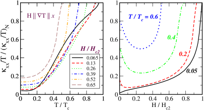
Figure 5: (Color online) Longitudinal heat conductivity for ${\bf H}||\mbox{\boldmath$\nabla$}T||\hat{x}$-antinodal direction: as a function of temperature for several fields (left); right: as a function of the field for temperatures {0.05, 0.2, 0.4, 0.6}.

We start by showing the temperature and field dependence of the heat conductivity tensor for the $d_{x^{2}-y^{2}}$ gap. The heat current and the field are along the ${\bf x}$-axis, along the gap maximum, as schematically shown in Fig. 3. The longitudinal thermal conductivity is seen in Fig. 5 to rapidly decrease below $T_{c}(H)$ (left panel), as the gap opens in the single-particle spectrum. Notice, however, that the lines plotted for different fields intersect, implying that the field dependence of $\kappa_{xx}$ is non-monotonic, as shown in the right panel. $\kappa_{xx}(H)$ increases with field at the lowest $T$ and $H$. In this regime the low energy quasiparticles are located near the gap nodes, where order parameter vanishes, ${\cal Y}(\phi_{n})=0$, and the transport lifetime, Eq.(27) is limited only by the impurity scattering, $-\mathfrak{Im}\,\Sigma^{R}$. Hence in the competition between the increased number of heat-carrying quasiparticles due to field and scattering on the vortices, the density of states wins, and the conductivity increases with field. In contrast, at higher $T$, the unpaired quasiparticles are already induced by temperature away from the nodes, and turning on the field leads to increased scattering, hence the decrease in the thermal conductivity. The evolution of $\kappa_{xx}$ with $T$ and $H$ is nearly identical to that found for the field normal to the layers in a vortex state model with a single Landau level Vekhter and Houghton (1999), and is in agreement with experimental results Matsuda et al. (2006).

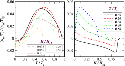
Figure 6: (Color online) Transverse heat conductivity for $\mbox{\boldmath$\nabla$}T||\hat{x}$-antinodal direction: ${\bf H}||node$ as a function of temperature (left) and field (right).

Fig. 6 shows the temperature (left panel) and field (right panel) dependence of the transverse heat conductivity. As we emphasized above, for a general orientation of the field the dominant contribution to the transverse heat conductivity is not caused by bending of the quasiparticle trajectories in the applied field due to Lorenz force, but is due instead to the anisotropic scattering of quasiparticles by the vortices. If the thermal gradient is not along one of these two “transport axes”, along the vortices and perpendicular to the vortices, transverse current arises. On the other hand, if the thermal gradient is along or normal to the field direction, $\kappa_{xy}=0$ by symmetry, as is clear from Eq. (30). Hence we show the transverse conductivity for $\phi_{0}=45^{\circ}$ which corresponds to ${\bf H}||node$.

The transverse conductivity is allowed to change sign, as it only reflects the difference between the thermal conductivities parallel and perpendicular to H, which themselves depend on the temperature and field. The temperature dependence shows a large peak at intermediate $T$ for all $H$ and tends to zero as the normal state is approached. The field dependence is more interesting. At low temperature, $\kappa_{xy}$ is negative and monotonically decreasing up to the critical field, and rapidly goes to zero at $H_{c2}$. At higher temperature $\kappa_{xy}$ is positive, and has a peak at low fields. The temperature, at which the peak first appears, seems correlated with that where the downturn in $\kappa_{xx}(H)$ is first seen, and the field value at the peak position moves in step with the minimum of $\kappa_{xx}(H)$ in Fig. 5 (right). It is therefore likely that this feature is a signature of the increased scattering due to magnetic field. This is supported by correlations between the peak and significant $\kappa(90^{\circ})-\kappa(0^{\circ})$, which stems from magnetic scattering.

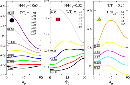
Figure 7: (Color online) Heat conductivity profiles for $T$-scans at two different fields and a $H$-scan at $T/T_{c}=0.25$. Different symbols correspond to points in Fig. 10 (left). The curves are shifted vertically to fit on the same plot, and the value for $\phi_{0}=0$ for each of the shifted curves is given in the corresponding boxes.

To make connection to experiment, in Fig. 7 we show the temperature scans of the longitudinal heat conductivity as a function of the field direction for low and moderate fields (left and middle panel respectively), and a field scan at $T/T_{c}=0.25$ (right panel). The evolution with temperature at low field is similar to that found for the cylindrical FS, see Fig. 3. The low temperature region is dominated by the evolution of the four-fold term, while, as temperature increases, the two-fold component becomes more prominent. The field scan strongly resembles the analogous result for the cylindrical FS: note the appearance of a pronounced peak for the nodal direction ($\phi_{0}=45^{\circ}$) with increasing field. This shape of $\kappa_{xx}(\phi_{0})$ strongly resembles the experimentally found anisotropy in CeCoIn₅ as shown in Ref.Izawa et al., 2001. This speaks in favor of the $d_{x^{2}-y^{2}}$ gap symmetry in this material, and we will provide the detailed analysis at the end of this section.

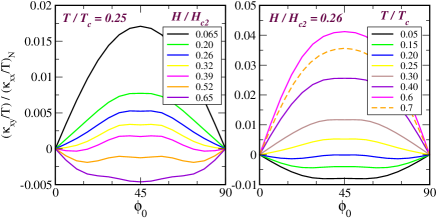
Figure 8: (Color online) Anisotropy profile of the transverse heat conductivity. This component gives the heat current along the $y$-direction, when the $\mbox{\boldmath$\nabla$}T||x$ and the field makes angle $\phi_{0}$ with the antinodal $x$-axis.

For the same relative orientation of the gap and the heat current, we show a typical profile of the transverse thermal conductivity, $\kappa_{xy}$, in Fig. 8. For $\phi_{0}=0^{\circ}$ and $\phi_{0}=90^{\circ}$ this component vanishes identically, see discussion above. Over a wide range of $T$ and $H$ parameter range this component shows essentially $\sin 2\phi_{0}$-like behavior Eq.(32) that agrees with experimental findings in high-$T_{c}$ materials.Ocaña and Esquinazi (2001, 2002) We emphasize that this modulation is completely unrelated to the nodal structure of the gap, moreover, only the deviation from the pure sinusoidal profile, seen in several curves in Fig. 8, carries information about the gap structure.

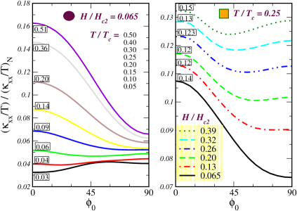
Figure 9: (Color online) Longitudinal heat conductivity anisotropy for $d_{xy}$ symmetry. The curves are shifted vertically, so the scale on the vertical axis shows only the absolute anisotropy. The relative anisotropy can be deduced from the true values of $\kappa_{xx}(0)$ shown in boxes. On the left is shown a temperature scan for $H/H_{c2}=0.065$, and on the right is a field scan for $T/T_{c}=0.25$, shown correspondingly by filled circles and squares in Fig. 10 (right).

To complete the description of the thermal conductivity, we present in Fig. 9 the longitudinal thermal conductivity $\kappa_{xx}(\phi_{0})$ for $d_{xy}$ symmetry of the order parameter (when the temperature gradient is along a nodal direction), and compare it with the results for the $d_{x^{2}-y^{2}}$ gap in Fig. 7. The temperature scans for field $H/H_{c2}=0.065$ in Fig. 7(a) and Fig. 9(left) demonstrate that at high temperatures the same two-fold symmetry holds for both gap symmetries. At low $T$ the fourfold feature disappears slightly faster for the $d_{xy}$ gap, and, at the lowest $T$, clearly has the opposite sign for the two gaps; this is in agreement with Eq.(32) and Eq.(37). Comparison of the field scans for $T/T_{c}=0.25$, Fig. 7(c) and Fig. 9(right), shows a rather dramatic difference between the profile of the thermal conductivity under the rotated field for the two cases. A local maximum for the field at $\phi_{0}=45^{\circ}$ to the heat current is clearly resolved for $d_{x^{2}-y^{2}}$ gap. For the same field direction either a minimum or no feature is seen for the $d_{xy}$ symmetry. Recall that at this temperature, $T\ll T_{c}$, the thermally excited quasiparticles are still located near the nodes of the gap, at $\phi_{n}$. Their scattering on the vortices depends on the component of the Fermi velocity normal to the field, and therefore on the sine of the angle between the nodal and the field directions. Hence the strongest variation in the scattering occurs as the field sweeps through the nodal direction, when $|\phi_{n}-\phi_{0}|\ll 1$. For the $d_{x^{2}-y^{2}}$ gap, with nodes at $\phi_{n}=45^{\circ}+n90^{\circ}$ to the direction of the heat current, this leads to a noticeable feature in the profile of the thermal conductivity for $\phi_{0}\simeq\phi_{n}$. For the $d_{xy}$ order parameter, with $\phi_{n}=n90^{\circ}$, the rotated field sweeps through the nodes at the same time as it is either parallel or normal to the heat current, $\phi_{0}\simeq 0^{\circ},90^{\circ}$. In that case the twofold transport anisotropy due to vortices masks the nodal signatures, and the signal is largely twofold. Only in restricted regions of the phase diagram, when the dominant twofold anisotropy is nearly absent (intermediate fields in the right panel of Fig. 9), does the existence of the nodes affect the profile of $\kappa_{xx}$. This difference between the behavior of $\kappa_{xx}(\phi_{0})$ for the two types of gap strongly suggests to us that the experimental results for CeCoIn₅ effectively rule out the $d_{xy}$ symmetry for this compound.

In Fig. 10 we summarize the results in the form of a phase diagram. The most noticeable differences with the cylindrical Fermi surface, Fig. 3, occur near the upper critical field due to the $H_{c2}$ anisotropy, absent in the non-self-consistent calculation. Away from the critical field, in the low-to-moderate $T$,$H$ corner, however, the anisotropy shows very similar features for the cylindrical and the corrugated FS, although the detailed positions of the separation lines, indicating the change in the shape of the thermal conductivity profile, is different. We believe that the location of these lines is determined by the symmetry and the shape of the Fermi surface, and other microscopic details of the material. Recall that the coupling between different Landau level components of the order parameter is generated by the action of the differential operator, ${\bf v}_{f}({\bf p})\cdot{\bm{\nabla}}$, which explicitly depends on the symmetries of the Fermi velocity. On the other hand, based on the similarities between the phase diagram computed with the lowest Landau level, Fig. 3, and that for three components, Fig. 10, we conclude that the salient features and changes in the anisotropy as a function of temperature and field are captured here.

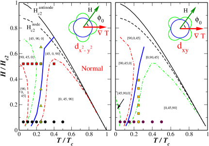
Figure 10: (Color online) The anisotropy phasediagram of the longitudinal heat conductivity $\kappa_{xx}(\phi_{0})$. Notation $[\phi_{0}^{a},\phi_{0}^{b},\phi_{0}^{c}]$ is short for $\kappa_{xx}(\phi_{0}^{a})>\kappa_{xx}(\phi_{0}^{b})>\kappa_{xx}(\phi_{0}^{c})$. The solid blue line corresponds to the change of sign in the $\kappa_{2}$, which is positive at high $T$ and negative at low $T$. Its position on the phase diagram is almost the same for the heat current along antinode and node. Left panel: the temperature gradient is along the antinodal direction. The symbols (circles, squares and triangles) correspond to anisotropy curves in Fig. 7. The variation of the transverse heat conductivity anisotropy for this gap orientation is shown in Fig. 8. Right panel: the temperature gradient is along a nodal direction.

It is also clear from the phase diagrams in Fig. 10 and the anisotropy profiles in Figs. 7 and 9 that there is no simple relation between general shape and evolution of $\kappa_{ij}(\phi_{0})$ for the two symmetries of the gap, $d_{x^{2}-y^{2}}$ and $d_{xy}$. On the other hand, as we noted earlier, the coefficient $\kappa_{4}$ in the Fourier decomposition analogous to Eq. (32) and suggested in Ref. Matsuda et al., 2006, $\kappa_{xx}(\phi_{0})=\kappa_{0}+\kappa_{2}\cos 2\phi_{0}+\kappa_{4}\cos 4\phi_{0}$, depends only on the orientation of the field with respect to the nodes. In Fig. 11 we plot the four-fold coefficient $\kappa_{4}$ for the values of $T$ and $H$ shown in Fig. 7 for the $d_{x^{2}-y^{2}}$ gap.

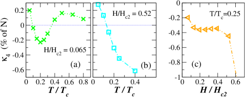
Figure 11: (Color online) The four-fold symmetry coefficient $\kappa_{4}$ of heat conductivity for the scans shown above in figure 7.

The four-fold anisotropy changes sign at intermediate temperatures for both small and moderate fields, see left two panels of Fig. 11. The coefficient $\kappa_{4}$ is small near $T_{c}$, where only the two-fold pattern that reflects the difference between transport parallel and normal to the applied field is detectable. The second sign change in the low-field range, left panel of Fig. 11, occurs at low temperature, close to the limit of validity of the BPT approximation Vorontsov and Vekhter (2007). However, it is this feature that is connected in the phase diagram to the reversal shown in the middle panel for higher fields, see Fig. 12, which suggests that it is not an artifact of the approach, but a real effect.

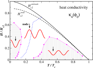
Figure 12: (Color online) The $T$-$H$ phase diagram for the fourfold component, $\kappa_{4}$, of the thermal conductivity under rotated magnetic field. Differently shaded regions correspond to different sign of the four-fold term, and its connection to the nodal directions. The dashed line marks the crossover from $\kappa_{xx}(0)<\kappa_{xx}(90^{\circ})$ at low $T$ to $\kappa_{xx}(0)>\kappa_{xx}(90^{\circ})$ at high $T$.

For the field scan at $T/T_{c}=0.25$ (right panels of Figs. 7,11) $\kappa_{4}$ is always negative, so that the minima in the four-fold component mark the antinodal directions, while the maxima occur for ${\bf H}$ along the nodes. There is a sharp increase in the magnitude of this coefficient as we approach the critical field due to the in-plane $H_{c2}$ anisotropy.

V.2 Comparison with experiment: CeCoIn₅ and $\kappa$-(BEDT-TTF)₂Cu(NCS)₂

We close this section with a detailed comparison of our results with the experimental data. One of the main motivations for this work was the measurement of the thermal conductivity in a heavy fermion CeCoIn₅,  Izawa et al. (2001). Another example of quasi-2D superconductor where the anisotropy was measured is $\kappa$-(BEDT-TTF)₂Cu(NCS)₂. Izawa et al. (2002a).

In CeCoIn₅ the heat current is driven along [100] crystal direction. The observed profile of the heat conductivity at $T/T_{c}=0.25$ is in good agreement with that shown in Fig. 7 ($d_{x^{2}-y^{2}}$) for comparable temperature ($T\approx 0.2T_{c}$), including the peak for the field at 45^∘ to the heat current. The profile differs significantly from that expected for a $d_{xy}$ gap as shown in Fig. 9. We find that the behavior of the experimentally determined four-fold term amplitude, $\kappa_{4}$, agrees with Fig. 11 (right): it vanishes as $H\to 0$ and saturates at $H\geq 0.2\,H_{c2}$. The overall amplitude of this component is smaller in our computation than that observed experimentally by approximately a factor of three: however, since this magnitude is determined by the shape of the Fermi surface, we do not expect the model calculation to be quantitatively correct. Our results at moderate temperatures are consistent with the experimental temperature scan $T=0.15-0.9\,T_{c}$ at $H\approx 0.1H_{c2}$. At $T\sim T_{c}$ our results suggest an inversion of the $\kappa_{4}$-term which was not observed. However, in this region CeCoIn₅ still has strong inelastic scattering (resulting in a peak of the thermal conductivity at $T\sim 0.75T_{c}$) which was not included in the calculation. Experimentally, extraction of the small $\kappa_{4}$ amplitude on the background of the dominant twofold term has greater relative errors. Moreover, since in this range $\kappa_{0}\gg\kappa_{2}\gg\kappa_{4}$, the difference between the calculated and the measured heat conductivity described in Sec. III.3 may also contribute to the discrepancy. Finally, since the upper critical field in CeCoIn₅ is paramagnetically limited, we cannot make a reliable connection of our results with experiment at low temperatures and high fields; in contrast, Zeeman splitting does not affect the low-to-intermediate $T$-$H$ behavior. Therefore reliable comparison can be made only in the region away from the critical field, where a maximum in the fourfold component points to the node, strongly implying $d_{x^{2}-y^{2}}$ symmetry in agreement with Ref. Izawa et al., 2001. Note that, according to our analysis, generally the line of inversion of the fourfold term in Fig. 12 is distinct from the line separating the increasing and decreasing $\kappa(H,T)$ at low fields, which was used to decide whether the minima or the maxima of the oscillations indicate the nodes in Ref. Izawa et al., 2001.

In the quasi-2D organic superconductor $\kappa$-(BEDT-TTF)₂Cu(NCS)₂ the available data are in low-$T,H$ region only Izawa et al. (2002a). The heat current is driven along [110] axis. Extensive analysis of the experimental data is required to separate the electronic contribution (which is small due low carrier density), from the phonon heat transport. If, however, we concentrate our attention only on the behavior of the four-fold electronic term, the observed anisotropy fits well into the phase diagram for the $d_{xy}$ gap, Fig. 10. In the region $H\sim 0.07H_{c2}$, $T=0.04-0.07T_{c}$, the fourfold term, $\kappa_{4}\cos 4\phi_{0}$, has a maximum for $\phi_{0}=0^{\circ}$ (along [110]) for $T\sim 0.04T_{c}$, and essentially disappears at $T\sim 0.07T_{c}$. In our mapping to the phase diagram, in the experimental regime the field along the node produces minima in the conductivity, and we concur with Ref. Izawa et al., 2002a that the nodal direction is [100], which suggests the $d_{xy}$ symmetry.

VI Conclusions

In this paper, following our approach in I for the specific heat, and using the non-equilibrium Keldysh formulation of the quasiclassical theory, we derived a general expression for the heat conductivity tensor of a superconductor in magnetic field. The derivation was based on the closed form solution for the Green’s function obtained in I, that made use of the Brandt-Pesch-Tewordt approximation. The utility of this approach lies in its ability to self-consistently take into account impurity scattering, the detailed shape of the Fermi surface, and multiple Landau levels in the order parameter in the vortex state. Numerical computations based on this approach are very time-efficient. The main advantage of our approach is that it provides unified method for calculations of transport and thermodynamics over a large range of temperatures and fields, well beyond the realm of applicability of the semiclassical schemes.

Figure 13: (Color online) The $T$-$H$ phase diagram for anisotropy of the heat capacity under rotated magnetic field. We choose for our model a quasi-cylindrical Fermi surface and a $d$-wave order parameter. For rotations of the field in the $ab$-plane the oscillations of the heat conductivity are four-fold, and a different feature (maximum or minimum) of this dependence determine the node position (arrows), depending on the location on this diagram.

In these two papers we applied the developed formalism to a $d$-wave superconductor with a quasi-cylindrical Fermi surface. We concentrated on the behavior of the specific heat and thermal conductivity, since they are the most widely used experimental probes. To make a connection between theory and experiment, we provided, for the first time, a complete description of the anisotropy of the thermal conductivity and specific heat in the $T$-$H$ phase diagram, starting from the “semiclassical” region at low $T,H$ and up to the critical field.

Two figures summarize the main results of this work. Figure 13 recalls the results of I, and shows the phase diagram for anisotropy of the specific heat under rotated magnetic field, $C(\phi_{0})$. The preceding figure, Fig. 12, shows the anisotropy of the fourfold component, $\kappa_{4}$, of the longitudinal thermal conductivity, $\kappa_{xx}$, for the model. One of our main findings is that both anisotropic signatures change sign, i.e. invert, in the $T$-$H$ plane. For the specific heat, the inversion of the anisotropy is due to the effect of the quasiparticle scattering on vortices on the density of states, see I. The semiclassical (Doppler shift) picture predicting a minimum of $C$ for the field along a node is valid at low $T$ and $H$, where it was designed to work. The effects of the energy shift, however, are superseded by the redistribution of the spectral weight due to scattering, which becomes dominant not only at moderate fields, but also at low fields for finite energies. Consequently, the anisotropy changes sign at finite $T$, Fig. 13.

Analysis of the heat conductivity is more involved due to interdependence of the transport scattering time and the density of states in the self-consistent treatment. We showed that, under a rotated field, the four-fold term in Fourier decomposition of the heat conductivity, $\kappa_{4}(\phi_{0})$, exhibits signatures of the nodes, and depends only on the angle between the field, ${\bf H}$, and the nodal directions, but not on the orientation of the heat current relative to the nodes. From comparison of Fig. 12 and Fig. 13 it is clear that the evolution of the fourfold coefficients in the specific heat and thermal conductivity, including sign changes, is quite similar across the phase diagram.

The exact location of the inversion lines depends on the microscopic details, such as the Fermi surface shape and the detailed structure of the order parameter. The relative position of these lines, however, is stable with respect to the moderate changes of the FS curvature along $z$-axis and impurity concentration. The developed theory is valid over most of the phase diagram, except for very low fields in dirty samples, where the averaging procedure in the Brandt-Pesch-Tewordt approximation is no longer valid. Thus the qualitative changes in the fourfold term at moderate fields, where the anisotropy is the most prominent, should be detectable experimentally (albeit may prove labor-intensive). One possible experimental approach to search for the node locations would be to measure anisotropy at several points in the phase diagram, in order to map out the evolution of the anisotropic contribution.

Finally, by comparing our results with available experimental data on the specific heat and thermal conductivity we concluded that the order parameter of heavy fermion material CeCoIn₅Izawa et al. (2001); Aoki et al. (2004) has $d_{x^{2}-y^{2}}$ symmetry, and reconciled the thermodynamic and transport measurements. Analysis of the thermal conductivity for organic superconductor $\kappa$-(BEDT-TTF)₂Cu(NCS)₂Izawa et al. (2002a) places it most likely into $d_{xy}$ family. We believe that our method, which allows detailed microscopic calculations for specific compounds, will enable unambiguous interpretation of the anisotropy in thermal and transport properties of unconventional superconductors, and will lead to maturing of this method as a tool for determining the nodal directions.

VII Acknowledgements

This work was partly done at KITP with support from NSF Grant PHY99-07949; and was also supported by the Board of Regents of Louisiana. We thank D. A. Browne, C. Capan, P. J. Hirschfeld, Y. Matsuda, and T. Sakakibara for discussions. I. V. is grateful to A. Houghton for encouragement during early stages of this work.

Appendix A Details of the heat conductivity derivation

Our approach allows to obtain an expression for thermal conductivity that generalizes previous results to the case of vortex state with multi-Landau level order parameter, and arbitrary impurity strength.

Keldysh diagram technique is formulated for 8$\times$8 Green’s function,Serene and Rainer (1983) which is traditionally split into three $4\times 4$ parts, Retarded (R), Advanced (A) and Keldysh (K):$\widehat{g}^{X}$, $X=\{R,A,K\}$,

$$\check{g}=\left(\begin{array}[]{cc}\widehat{g}^{R}&\widehat{g}^{K}\\ 0&\widehat{g}^{A}\end{array}\right)\,,$$ (47)

$$\widehat{g}^{X}(\hat{{\bf p}},{\bf R};\varepsilon)=\left(\begin{array}[]{cc}g^{X}+{\bf g}^{X}\mbox{\boldmath$\sigma$}&(f^{X}+{\bf f}^{X}\mbox{\boldmath$\sigma$})i\sigma_{2}\\ i\sigma_{2}(\underline{f}^{X}+\underline{{\bf f}}^{X}\mbox{\boldmath$\sigma$})&\underline{g}^{X}+\underline{{\bf g}}^{X}\mbox{\boldmath$\sigma$}^{*}\end{array}\right)$$ (48)

For stationary problems these functions obey the normalization conditions:

$$\widehat{g}^{R,A}\widehat{g}^{R,A}=-\pi^{2}\hat{1}\qquad\,,\qquad\widehat{g}^{R}\widehat{g}^{K}+\widehat{g}^{K}\widehat{g}^{A}=0.$$ (49)

We do not need to solve equations for all the functions as they are related through symmetries,Serene and Rainer (1983)

$$\begin{array}[]{c@{\quad}c}g^{R}(\hat{{\bf p}};\varepsilon)=g^{A}(\hat{{\bf p}};\varepsilon)^{*}&{\bf g}^{R}(\hat{{\bf p}};\varepsilon)={\bf g}^{A}(\hat{{\bf p}};\varepsilon)^{*}\\ g^{R}(\hat{{\bf p}};\varepsilon)=\underline{g}^{A}(-\hat{{\bf p}};-\varepsilon)&{\bf g}^{R}(\hat{{\bf p}};\varepsilon)=\underline{{\bf g}}^{A}(-\hat{{\bf p}};-\varepsilon)\\ g^{K}(\hat{{\bf p}};\varepsilon)=\underline{g}^{K}(-\hat{{\bf p}};-\varepsilon)&{\bf g}^{K}(\hat{{\bf p}};\varepsilon)=\underline{{\bf g}}^{K}(-\hat{{\bf p}};-\varepsilon)\end{array}$$ (50)

$$\begin{array}[]{c@{\quad}c}f^{R}(\hat{{\bf p}};\varepsilon)=\underline{f}^{A}(\hat{{\bf p}};\varepsilon)^{*}&{\bf f}^{R}(\hat{{\bf p}};\varepsilon)=\underline{{\bf f}}^{A}(\hat{{\bf p}};\varepsilon)^{*}\\ f^{R}(\hat{{\bf p}};\varepsilon)={f}^{A}(-\hat{{\bf p}};-\varepsilon)&{\bf f}^{R}(\hat{{\bf p}};\varepsilon)={{\bf f}}^{A}(-\hat{{\bf p}};-\varepsilon)\\ f^{K}(\hat{{\bf p}};\varepsilon)=-\underline{f}^{K}(\hat{{\bf p}};\varepsilon)^{*}&{\bf f}^{K}(\hat{{\bf p}};\varepsilon)=-\underline{{\bf f}}^{K}(\hat{{\bf p}};\varepsilon)^{*}\end{array}$$ (51)

The different functions obey transport equations:

$$[(\varepsilon-\sigma_{B})\widehat{\tau}_{3}-\widehat{\sigma}^{R,A},\widehat{g}^{R,A}]+i{\bf v}_{f}\mbox{\boldmath$\nabla$}\widehat{g}^{R,A}=0$$ (52)

$$((\varepsilon-\sigma_{B})\widehat{\tau}_{3}-\widehat{\sigma}^{R})\widehat{g}^{K}-\widehat{g}^{K}((\varepsilon-\sigma_{B})\widehat{\tau}_{3}-\widehat{\sigma}^{A})$$

$$\hskip 28.45274pt-\widehat{\sigma}^{K}\widehat{g}^{R}+\widehat{g}^{A}\widehat{\sigma}^{K}+i{\bf v}_{f}\mbox{\boldmath$\nabla$}\widehat{g}^{K}=0\,.$$ (53)

Here

$$\sigma_{B}=-{e\over c}{\bf v}_{f}{\bf A}\,,$$ (54)

is the coupling of quasiparticles to an external magnetic field. The self-energy is decomposed into the mean-filed order parameter and the impurity contributions, $\widehat{\sigma}^{X}=\widehat{\Delta}^{X}+\widehat{\sigma}^{X}_{imp}$. Self-consistency equations for the singlet order parameter are

$$\Delta^{R}({\bf p},{\bf R})=\Delta^{A}({\bf p},{\bf R})=$$ (55)

$$\hskip 28.45274pt=\int\limits_{-\infty}^{+\infty}{d\varepsilon\over 4\pi i}\int d\hat{{\bf p}}^{\prime}n_{f}(\hat{{\bf p}}^{\prime})V_{s}({\bf p},{\bf p}^{\prime})f^{K}({\bf p}^{\prime},{\bf R};\varepsilon)\,,$$

$$\Delta^{K}({\bf p},{\bf R})=0\,,$$ (56)

and for triplet superconductivity the equations are identical, upon replacing $\Delta^{X}$ by its vector counterpart, $\mbox{\boldmath$\Delta$}^{X}$. The Keldysh part of the self-energy comes in this case from impurities only. The self-consistent t-matrix approximation for isotropic impurity scattering gives

$$\widehat{\sigma}^{X}_{imp}({\bf R};\varepsilon)=n_{imp}\widehat{t}^{X}({\bf R};\varepsilon)$$ (57)

$$\widehat{t}^{R,A}=u\hat{1}+uN_{f}\langle\widehat{g}^{R,A}\rangle\widehat{t}^{R,A}$$ (58)

$$\widehat{t}^{K}=N_{f}\widehat{t}^{R}\langle\widehat{g}^{K}\rangle\widehat{t}^{A}$$ (59)

where the angular brackets denote the normalized Fermi surface average as in the main text of the paper.

In this appendix we denote functions in thermal equilibrium by the subscript ‘eq’, but in the main text we omit it for brevity. In local equilibrium,

$$\widehat{g}_{\mbox{\tiny eq}}^{K}=\widehat{g}_{\mbox{\tiny eq}}^{R}\Phi_{\mbox{\tiny eq}}-\Phi_{\mbox{\tiny eq}}\widehat{g}_{\mbox{\tiny eq}}^{A}\;,\;\widehat{\sigma}_{\mbox{\tiny eq}}^{K}=\widehat{\sigma}_{\mbox{\tiny eq}}^{R}\Phi_{\mbox{\tiny eq}}-\Phi_{\mbox{\tiny eq}}\widehat{\sigma}_{\mbox{\tiny eq}}^{A}\,,$$ (60)

$$\Phi_{\mbox{\tiny eq}}=\tanh\left({\varepsilon\over 2T({\bf R})}\right)\,.$$ (61)

Heat current is

$${\bf j}_{h}({\bf R})=2N_{f}\int d{\bf p}_{f}n_{f}({\bf p}_{f})\int\limits_{-\infty}^{+\infty}{d\varepsilon\over 4\pi i}\varepsilon{\bf v}_{f}({\bf p}_{f})g^{K}({\bf p}_{f},{\bf R};\varepsilon)\,,$$ (62)

where $g^{K}({\bf p}_{f},{\bf R};\varepsilon)$ is the diagonal part of $\widehat{g}^{K}$. Using the Green’s function symmetries one can show that in this formula it is equivalent to $g^{K}=1/4\,\mbox{Tr}(\widehat{g}^{K})$. The factor of two reflects our definition of $N_{f}$ for single spin projection. Thermal conductivity in the linear response is determined from

$$\delta{\bf j}_{h}({\bf R})\equiv-\hat{\kappa}\,\mbox{\boldmath$\nabla$}T=$$ (63)

$$=2N_{f}\int d{\bf p}_{f}n_{f}({\bf p}_{f})\int\limits_{-\infty}^{+\infty}{d\varepsilon\over 4\pi i}\varepsilon{\bf v}_{f}({\bf p}_{f})\,{1\over 4}\mbox{Tr}[\delta g^{K}({\bf p}_{f},{\bf R};\varepsilon)]\,.$$

Our goal is to find the linear, in the temperature gradient that drives the heat current, correction to the Keldysh Green’s function, $\delta g^{K}$. The Green’s functions varies on the scale of the magnetic length (or intervortex distance), $\Lambda$, and on the scale of the superconducting coherence length, $\xi_{0}$. We assume that $\Lambda,\xi_{0}\ll L_{T}$, where $L_{T}$ is the length scale for temperature variation. We now write the gradient term as a sum of the gradients due to inhomogeneity and due to the externally imposed slow temperature variation,

$$\mbox{\boldmath$\nabla$}=\mbox{\boldmath$\nabla$}_{x}+\mbox{\boldmath$\nabla$}T\;\frac{\partial}{\partial T}\,,$$ (64)

with the last term much smaller than the first.

Solution in the local equilibrium is obtained from

$$[\widehat{h}_{\mbox{\tiny eq}}^{R,A},\widehat{g}_{\mbox{\tiny eq}}^{R,A}]+i{\bf v}_{f}\mbox{\boldmath$\nabla$}_{x}\widehat{g}^{R,A}_{\mbox{\tiny eq}}=0$$

$$\widehat{h}_{\mbox{\tiny eq}}^{R,A}=(\varepsilon-\sigma_{B})\widehat{\tau}_{3}-\widehat{\sigma}^{R,A}_{\mbox{\tiny eq}}\,.$$ (65)

We note that the following analysis can be easily adjusted if we add an external potential to $\widehat{h}_{\mbox{\tiny eq}}^{R,A}$. For now we continue without it and write down linearized equations for Green’s functions near equilibrium, $\widehat{g}^{X}=\widehat{g}^{X}_{\mbox{\tiny eq}}+\delta\widehat{g}^{X}$, with driving term due to ${\bf v}_{f}\mbox{\boldmath$\nabla$}_{T}\equiv{\bf v}_{f}\,\mbox{\boldmath$\nabla$}T\,\partial_{T}$,

$$[\widehat{h}_{\mbox{\tiny eq}}^{R,A},\delta\widehat{g}^{R,A}]+[-\delta\widehat{\sigma}^{R,A},\widehat{g}_{\mbox{\tiny eq}}^{R,A}]+i{\bf v}_{f}\mbox{\boldmath$\nabla$}_{x}(\delta\widehat{g}^{R,A})+i{\bf v}_{f}\mbox{\boldmath$\nabla$}_{T}\,\widehat{g}_{\mbox{\tiny eq}}^{R,A}=0$$ (66)

$$\widehat{h}_{\mbox{\tiny eq}}^{R}\delta\widehat{g}^{K}-\delta\widehat{g}^{K}\widehat{h}_{\mbox{\tiny eq}}^{A}-\delta\widehat{\sigma}^{R}\widehat{g}_{\mbox{\tiny eq}}^{K}+\widehat{g}_{\mbox{\tiny eq}}^{K}\delta\widehat{\sigma}^{A}-\delta\widehat{\sigma}^{K}\widehat{g}_{\mbox{\tiny eq}}^{A}+\widehat{g}_{\mbox{\tiny eq}}^{R}\delta\widehat{\sigma}^{K}-\widehat{\sigma}_{\mbox{\tiny eq}}^{K}\delta\widehat{g}^{A}+\delta\widehat{g}^{R}\widehat{\sigma}_{\mbox{\tiny eq}}^{K}$$

$$\hskip 227.62204pt+i{\bf v}_{f}\mbox{\boldmath$\nabla$}_{x}(\delta\widehat{g}^{K})+i{\bf v}_{f}\mbox{\boldmath$\nabla$}_{T}\,\widehat{g}_{\mbox{\tiny eq}}^{K}=0$$ (67)

We decouple equations for $\delta\widehat{g}^{R,A}$ from $\delta\widehat{g}^{K}$ by introducing Eliashberg anomalous propagatorRainer and Sauls (1995); Graf et al. (1996) and the self-energy,

$$\delta\widehat{g}^{K} = \delta\widehat{g}^{R}\Phi_{\mbox{\tiny eq}}-\Phi_{\mbox{\tiny eq}}\delta\widehat{g}^{A}+\delta\widehat{g}^{a}\,,$$ (68)

$$\delta\widehat{\sigma}^{K} = \delta\widehat{\sigma}^{R}\Phi_{\mbox{\tiny eq}}-\Phi_{\mbox{\tiny eq}}\delta\widehat{\sigma}^{A}+\delta\widehat{\sigma}^{a}\,.$$ (69)

The heat current is determined by $\delta\widehat{g}^{a}$, which satisfies

$$\widehat{h}_{\mbox{\tiny eq}}^{R}\delta\widehat{g}^{a} - \delta\widehat{g}^{a}\widehat{h}_{\mbox{\tiny eq}}^{A}+i{\bf v}_{f}\mbox{\boldmath$\nabla$}_{x}\,\delta\widehat{g}^{a}=$$

$$= -i{\bf v}_{f}\mbox{\boldmath$\nabla$}_{T}\Phi_{\mbox{\tiny eq}}\;(\widehat{g}_{\mbox{\tiny eq}}^{R}-\widehat{g}_{\mbox{\tiny eq}}^{A})+\delta\widehat{\sigma}^{a}\widehat{g}_{\mbox{\tiny eq}}^{A}-\widehat{g}_{\mbox{\tiny eq}}^{R}\delta\widehat{\sigma}^{a}\,.$$

We need to solve this equation together with the self-consistency equations on $\delta\widehat{\sigma}^{X}$. Normalization requires

$$\widehat{g}^{R,A}_{\mbox{\tiny eq}}\,\delta\widehat{g}^{R,A}+\delta\widehat{g}^{R,A}\,\widehat{g}^{R,A}_{\mbox{\tiny eq}}=0\,,$$ (71)

$$\widehat{g}_{\mbox{\tiny eq}}^{R}\,\delta\widehat{g}^{a}+\delta\widehat{g}^{a}\,\widehat{g}_{\mbox{\tiny eq}}^{A}=0\,.$$ (72)

Up to this point all the equations are valid for both singlet and triplet pairing states. Below we focus on the singlet pairing and only briefly comment on the differences between the singlet and the triplet cases. The self-consistency for the retarded and advanced linear corrections contain the order parameter and the impurity contributions, $\delta\widehat{\sigma}^{R,A}=\delta\widehat{\Delta}+\delta\widehat{\sigma}^{R,A}_{imp}$, with

$$\delta\Delta=\int{d\varepsilon\over 4\pi i}\int d{\bf p}^{\prime}n_{f}({\bf p}^{\prime})V({\bf p},{\bf p}^{\prime})\;\delta f^{K}({\bf p}^{\prime},{\bf R};\varepsilon)$$ (73)

$$\delta\widehat{\sigma}_{imp}^{R,A}=n_{imp}N_{f}\,\widehat{t}^{R,A}_{\mbox{\tiny eq}}\langle\delta\widehat{g}^{R,A}\rangle\widehat{t}^{R,A}_{\mbox{\tiny eq}}\,,$$ (74)

but the anomalous part is due to impurities only,

$$\delta\widehat{\sigma}_{imp}^{a}=n_{imp}N_{f}\,\widehat{t}^{R}_{\mbox{\tiny eq}}\langle\delta\widehat{g}^{a}\rangle\widehat{t}^{A}_{\mbox{\tiny eq}}$$ (75)

We see that the equations for the anomalous Green’s function, $\delta\widehat{g}^{a}$, and the self-energy, $\delta\widehat{\sigma}^{a}$, are completely decoupled from those for the retarded and advanced Green’s functions. On the other hand, the equations for $\delta\widehat{g}^{R,A}$ depend on the anomalous $\delta\widehat{g}^{a}$ through the variation $\delta\Delta$. For simple retarded and advanced Green’s function ($Y=R,A$),

$$\widehat{g}^{Y}_{\mbox{\tiny eq}}=\left(\begin{array}[]{cc}g^{Y}_{\mbox{\tiny eq}}&f^{Y}_{\mbox{\tiny eq}}i\sigma_{2}\\ i\sigma_{2}\underline{f}^{Y}_{\mbox{\tiny eq}}&-g^{Y}_{\mbox{\tiny eq}}\end{array}\right)$$ (76)

we obtain the impurity t-matrix in equilibrium,

$$\widehat{t}^{Y}_{\mbox{\tiny eq}}=\left(\begin{array}[]{cc}t_{+}+t_{-}&t_{\Delta}\,i\sigma_{2}\\ i\sigma_{2}\,\underline{t}_{\Delta}&t_{+}-t_{-}\end{array}\right)={1\over n_{imp}}\frac{\Gamma\sin^{2}\delta_{0}}{1-{\sin^{2}\delta_{0}\over\pi^{2}}(\langle g_{\mbox{\tiny eq}}^{Y}\rangle^{2}-\overline{\langle f_{\mbox{\tiny eq}}^{Y}\rangle\langle\underline{f}_{\mbox{\tiny eq}}^{Y}\rangle}+\pi^{2})}\left(\begin{array}[]{cc}\mbox{ctg}\delta_{0}+\langle g_{\mbox{\tiny eq}}^{Y}\rangle/\pi&(\langle f_{\mbox{\tiny eq}}^{Y}\rangle/\pi)\,i\sigma_{2}\\ i\sigma_{2}\,(\langle\underline{f}_{\mbox{\tiny eq}}^{Y}\rangle/\pi)&\mbox{ctg}\delta_{0}-\langle g_{\mbox{\tiny eq}}^{Y}\rangle/\pi\end{array}\right)\,.$$ (77)

Here we solved (58) using the BPT approximation. Note that for the triplet case the off-diagonal parts $\langle f_{\mbox{\tiny eq}}\rangle$ vanish due to inversion symmetry, $\hat{{\bf p}}\to-\hat{{\bf p}}$.

For the singlet case we assume $\delta\widehat{\sigma}^{a}=0$, and validate this assumption at the end of the calculation. We show that the linear correction, $\delta\widehat{g}^{a}$, a product of an even, under $\hat{{\bf p}}\to-\hat{{\bf p}}$ reflection, function and an odd, in momentum, term ${\bf v}_{f}(\hat{{\bf p}})\mbox{\boldmath$\nabla$}_{T}$, so that its average over the FS vanishes.

We only need to solve the equation for the anomalous part of the Green’s function, since neither Retarded nor Advanced part has a unit-diagonal term. Hence $\mbox{Tr}[\widehat{g}^{R,A}]=0$, and they do not contribute to the heat current. Now $\mbox{Tr}[\delta\widehat{g}^{K}]=\mbox{Tr}[\delta\widehat{g}^{a}]$, and we find

$$\widehat{h}_{\mbox{\tiny eq}}^{R}\delta\widehat{g}^{a} - \delta\widehat{g}^{a}\widehat{h}_{\mbox{\tiny eq}}^{A}+i{\bf v}_{f}\mbox{\boldmath$\nabla$}_{x}\delta\widehat{g}^{a}=$$ (78)

$$= -i{\bf v}_{f}\mbox{\boldmath$\nabla$}_{T}\Phi_{\mbox{\tiny eq}}\;(\widehat{g}_{\mbox{\tiny eq}}^{R}-\widehat{g}_{\mbox{\tiny eq}}^{A})$$

where the matrix,

$$\widehat{h}_{\mbox{\tiny eq}}^{R,A} = (\varepsilon-\Sigma^{R,A}_{\mbox{\tiny eq}}-\sigma_{B})\hat{\tau}_{3}-D^{R,A}_{\mbox{\tiny eq}}\hat{1}-\widehat{\widetilde{\Delta}}^{R,A}_{\mbox{\tiny eq}}=$$ (79)

$$= \tilde{\varepsilon}^{R,A}\hat{\tau}_{3}-D^{R,A}_{\mbox{\tiny eq}}\hat{1}-\widehat{\widetilde{\Delta}}^{R,A}_{\mbox{\tiny eq}}\,,$$

depends only on the equilibrium self-energies, ($\widetilde{\mbox{\boldmath$\Delta$}}^{R,A}_{\mbox{\tiny eq}}=\mbox{\boldmath$\Delta$}_{\mbox{\tiny eq}}$ for a triplet)

$$\tilde{\varepsilon}^{R,A}=\varepsilon-\Sigma^{R,A}_{\mbox{\tiny eq}}-\sigma_{B}\,,$$ (80)

$$D^{R,A}_{\mbox{\tiny eq}}=n_{imp}t^{R,A}_{+}\,,$$ (81)

$$\Sigma^{R,A}_{\mbox{\tiny eq}}=n_{imp}t^{R,A}_{-}\,,$$ (82)

$$\widetilde{\Delta}^{R,A}_{\mbox{\tiny eq}}=\Delta_{\mbox{\tiny eq}}+n_{imp}t^{R,A}_{\Delta}\,.$$ (83)

We parameterize the anomalous propagator as

$$\delta\widehat{g}^{a}=\left(\begin{array}[]{cc}g^{a}+g^{\prime a}&f^{a}i\sigma_{2}\\ i\sigma_{2}\underline{f}^{a}&g^{a}-g^{\prime a}\end{array}\right)\,,$$ (84)

and find the equations for the diagonal components, $g^{a}$ and $g^{\prime a}$, from (78)

$$-g^{a}D^{a}+g^{\prime a}(\tilde{\varepsilon}^{R}-\tilde{\varepsilon}^{A})+{1\over 2}f^{a}(\underline{\widetilde{\Delta}}^{R}_{\mbox{\tiny eq}}-\underline{\widetilde{\Delta}}^{A}_{\mbox{\tiny eq}})+{1\over 2}\underline{f}^{a}(\widetilde{\Delta}^{R}_{\mbox{\tiny eq}}-\widetilde{\Delta}^{A}_{\mbox{\tiny eq}})+i{\bf v}_{f}\mbox{\boldmath$\nabla$}_{x}\,g^{a}=0\,,$$ (85)

$$-g^{\prime a}D^{a}+g^{a}(\tilde{\varepsilon}^{R}-\tilde{\varepsilon}^{A})-{1\over 2}f^{a}(\underline{\widetilde{\Delta}}^{R}_{\mbox{\tiny eq}}+\underline{\widetilde{\Delta}}^{A}_{\mbox{\tiny eq}})+{1\over 2}\underline{f}^{a}(\widetilde{\Delta}^{R}_{\mbox{\tiny eq}}+\widetilde{\Delta}^{A}_{\mbox{\tiny eq}})+i{\bf v}_{f}\mbox{\boldmath$\nabla$}_{x}\,g^{\prime a}=-i{\bf v}_{f}\mbox{\boldmath$\nabla$}_{T}\,\Phi_{\mbox{\tiny eq}}\;(g_{\mbox{\tiny eq}}^{R}-g_{\mbox{\tiny eq}}^{A})\,,$$ (86)

where we defined $D^{a}=D^{R}_{\mbox{\tiny eq}}-D^{A}_{\mbox{\tiny eq}}$. Expressions for the off-diagonal terms are obtained from the normalization condition (72),

$$f^{a}={1\over g^{R}_{\mbox{\tiny eq}}-g_{\mbox{\tiny eq}}^{A}}(-g^{a}(f_{\mbox{\tiny eq}}^{R}+f_{\mbox{\tiny eq}}^{A})+g^{\prime a}(f_{\mbox{\tiny eq}}^{R}-f_{\mbox{\tiny eq}}^{A}))$$ (87)

$$\underline{f}^{a}={1\over g^{R}_{\mbox{\tiny eq}}-g_{\mbox{\tiny eq}}^{A}}(g^{a}(\underline{f}_{\mbox{\tiny eq}}^{R}+\underline{f}_{\mbox{\tiny eq}}^{A})+g^{\prime a}(\underline{f}_{\mbox{\tiny eq}}^{R}-\underline{f}_{\mbox{\tiny eq}}^{A}))$$ (88)

Combining these equations, and using the BPT approximation (i.e. assuming that $g^{a},g^{\prime a}=$const and spatially averaging the terms containing $f$, $\underline{f}$ and $\Delta$), we obtain the final expression for the unit-diagonal part of the anomalous propagator,

$$g^{a}=\frac{G_{2}}{G_{1}G_{4}-G_{2}G_{3}}(g_{\mbox{\tiny eq}}^{R}-g_{\mbox{\tiny eq}}^{A})(i{\bf v}_{f}\mbox{\boldmath$\nabla$}\Phi_{\mbox{\tiny eq}})\,,$$ (89)

with the following definitions of coefficients,

$$G_{1} = -D^{a}+\frac{1}{2(g_{\mbox{\tiny eq}}^{R}-g_{\mbox{\tiny eq}}^{A})}\,\overline{[-(f_{\mbox{\tiny eq}}^{R}+f_{\mbox{\tiny eq}}^{A})(\underline{\widetilde{\Delta}}^{R}_{\mbox{\tiny eq}}-\underline{\widetilde{\Delta}}^{A}_{\mbox{\tiny eq}})+(\underline{f}_{\mbox{\tiny eq}}^{R}+\underline{f}_{\mbox{\tiny eq}}^{A})(\widetilde{\Delta}^{R}_{\mbox{\tiny eq}}-\widetilde{\Delta}^{A}_{\mbox{\tiny eq}})]}$$ (90)

$$G_{2} = \tilde{\varepsilon}^{R}-\tilde{\varepsilon}^{A}+\frac{1}{2(g_{\mbox{\tiny eq}}^{R}-g_{\mbox{\tiny eq}}^{A})}\,\overline{[(f_{\mbox{\tiny eq}}^{R}-f_{\mbox{\tiny eq}}^{A})(\underline{\widetilde{\Delta}}^{R}_{\mbox{\tiny eq}}-\underline{\widetilde{\Delta}}^{A}_{\mbox{\tiny eq}})+(\underline{f}_{\mbox{\tiny eq}}^{R}-\underline{f}_{\mbox{\tiny eq}}^{A})(\widetilde{\Delta}^{R}_{\mbox{\tiny eq}}-\widetilde{\Delta}^{A}_{\mbox{\tiny eq}})]}$$ (91)

$$G_{3} = \tilde{\varepsilon}^{R}-\tilde{\varepsilon}^{A}+\frac{1}{2(g_{\mbox{\tiny eq}}^{R}-g_{\mbox{\tiny eq}}^{A})}\,\overline{[(f_{\mbox{\tiny eq}}^{R}+f_{\mbox{\tiny eq}}^{A})(\underline{\widetilde{\Delta}}^{R}_{\mbox{\tiny eq}}+\underline{\widetilde{\Delta}}^{A}_{\mbox{\tiny eq}})+(\underline{f}_{\mbox{\tiny eq}}^{R}+\underline{f}_{\mbox{\tiny eq}}^{A})(\widetilde{\Delta}^{R}_{\mbox{\tiny eq}}+\widetilde{\Delta}^{A}_{\mbox{\tiny eq}})]}$$ (92)

$$G_{4} = -D^{a}+\frac{1}{2(g_{\mbox{\tiny eq}}^{R}-g_{\mbox{\tiny eq}}^{A})}\,\overline{[-(f_{\mbox{\tiny eq}}^{R}-f_{\mbox{\tiny eq}}^{A})(\underline{\widetilde{\Delta}}^{R}_{\mbox{\tiny eq}}+\underline{\widetilde{\Delta}}^{A}_{\mbox{\tiny eq}})+(\underline{f}_{\mbox{\tiny eq}}^{R}-\underline{f}_{\mbox{\tiny eq}}^{A})(\widetilde{\Delta}^{R}_{\mbox{\tiny eq}}+\widetilde{\Delta}^{A}_{\mbox{\tiny eq}})]}\,.$$ (93)

In order to prove that our assumption of $\delta\widehat{\sigma}^{a}=0$ is justified, we note that the coefficients $G_{i}$ are even under inversion of $\hat{{\bf p}}$. Then the resulting $g^{a}$ and $g^{\prime a}$ are odd due to additional factor ${\bf v}_{f}\mbox{\boldmath$\nabla$}\Phi_{\mbox{\tiny eq}}$, and their averages over the Fermi surface vanishes. The same is true for the off-diagonal functions $f^{a}$ and $\underline{f}^{a}$ in singlet case. This assumption is not valid for triplet pairing: even though $g^{a}$ and $g^{\prime a}$ are odd under inversion of $\hat{{\bf p}}$, we see from Eqs.(87) and (88) that $f^{a}$ and $\underline{f}^{a}$ are even (since $f_{\mbox{\tiny eq}}$’s are odd), and additional terms due to $\delta\widehat{\sigma}^{a}$ appear, making the self-consistent solution of the equations more difficult. Exceptions to this statement exist for certain order parameters and for special orientation of the temperature gradient. For example, when $\mbox{\boldmath$\nabla$}T$ is applied in a direction along which ${\bm{\Delta}}$ does not change, we find $\langle f^{a}\rangle=0$. Two obvious examples are a) $\mbox{\boldmath$\Delta$}(p_{z})$ and $\mbox{\boldmath$\nabla$}T$ is in the $xy$-plane and b) $\mbox{\boldmath$\Delta$}(p_{x},p_{y})$ and $\mbox{\boldmath$\nabla$}T\,||\,z$. )

The resulting expression for the heat conductivity is

$${\kappa_{ij}\over T}=\frac{N_{f}}{4\pi}\int{d\varepsilon\over T}\left(\frac{\varepsilon^{2}}{T^{2}\cosh^{2}(\varepsilon/2T)}\right)\int d{\bf p}_{f}\,n_{f}({\bf p}_{f})(v_{f,i}(\hat{{\bf p}})v_{f,j}(\hat{{\bf p}}))\frac{G_{2}}{G_{1}G_{4}-G_{2}G_{3}}(g_{\mbox{\tiny eq}}^{R}-g_{\mbox{\tiny eq}}^{A})\,.$$ (94)

We checked that this expression for a uniform superconductor agrees with the heat conductivity of Graf et al. Graf et al. (1996). This completes the derivation of the heat current. We remind the readers that in the main text we drop the equilibrium subscript ‘eq’ to make expressions less cluttered.

References

- Vorontsov and Vekhter (2007) A. Vorontsov and I. Vekhter, previous paper (unpublished).
- Vekhter et al. (1999) I. Vekhter, P. J. Hirschfeld, E. J. Nicol, and J. P. Carbotte, Phys. Rev. B 59, R9023 (1999).
- Park et al. (2003) T. Park, M. B. Salamon, E. M. Choi, H. J. Kim, and S.-I. Lee, Phys. Rev. Lett. 90, 177001 (2003).
- Park et al. (2004) T. Park, E. E. M. Chia, M. B. Salamon, E. D. Bauer, I. Vekhter, J. D. Thompson, E. M. Choi, H. J. Kim, S.-I. Lee, and P. C. Canfield, Phys. Rev. Lett. 92, 237002 (2004).
- Aoki et al. (2004) H. Aoki, T. Sakakibara, H. Shishido, R. Settai, Y. Onuki, P. Miranović, and K. Machida, Journal of Physics: Condensed Matter 16, L13 (2004).
- Park and Salamon (2004) T. Park and M. B. Salamon, Mod. Phys. Lett. B 18, 1205 (2004).
- Yu et al. (1995) F. Yu, M. B. Salamon, A. J. Leggett, W. C. Lee, and D. M. Ginsberg, Phys. Rev. Lett. 74, 5136 (1995), [Erratum ibid. 75, 3028].
- Aubin et al. (1997) H. Aubin, K. Behnia, M. Ribault, R. Gagnon, and L. Taillefer, Phys. Rev. Lett. 78, 2624 (1997).
- Watanabe et al. (2004) T. Watanabe, K. Izawa, Y. Kasahara, Y. Haga, Y. Onuki, P. Thalmeier, K. Maki, and Y. Matsuda, Phys. Rev. B 70, 184502 (2004).
- Izawa et al. (2001) K. Izawa, H. Yamaguchi, Y. Matsuda, H. Shishido, R. Settai, and Y. Onuki, Phys. Rev. Lett. 87, 057002 (2001).
- Izawa et al. (2003) K. Izawa, Y. Nakajima, J. Goryo, Y. Matsuda, S. Osaki, H. Sugawara, H. Sato, P. Thalmeier, and K. Maki, Phys. Rev. Lett. 90, 117001 (2003).
- Izawa et al. (2002a) K. Izawa, H. Yamaguchi, T. Sasaki, and Y. Matsuda, Phys. Rev. Lett. 88, 027002 (2002a).
- Izawa et al. (2002b) K. Izawa, K. Kamata, Y. Nakajima, Y. Matsuda, T. Watanabe, M. Nohara, H. Takagi, P. Thalmeier, and K. Maki, Phys. Rev. Lett. 89, 137006 (2002b).
- Matsuda et al. (2006) Y. Matsuda, K. Izawa, and I. Vekhter, J.Phys.: Cond.Mat. 18, R705 (2006).
- Won et al. (2005) H. Won, S. Haas, D. Parker, S. Telang, A. Vanyolos, and K. Maki, eprint cond-mat/0501463, (unpublished).
- Kübert and Hirschfeld (1998) C. Kübert and P. J. Hirschfeld, Phys. Rev. Lett. 80, 4963 (1998).
- Vekhter and Hirschfeld (2000) I. Vekhter and P. J. Hirschfeld, Physica C 341-348, 1947 (2000).
- Brandt et al. (1967) U. Brandt, W. Pesch, and L. Tewordt, Z. Phys. 201, 209 (1967).
- Pesch (1975) W. Pesch, Z. Phys. B 21, 263 (1975).
- Vorontsov and Vekhter (2006) A. B. Vorontsov and I. Vekhter, Phys. Rev. Lett. 96, 237001 (2006).
- Eilenberger (1968) G. Eilenberger, Z. Phys. 214, 195 (1968).
- Larkin and Ovchinnikov (1969) A. I. Larkin and Y. N. Ovchinnikov, Sov. Phys. JETP 28, 1200 (1969).
- Serene and Rainer (1983) J. W. Serene and D. Rainer, Phys. Rep. 101, 221 (1983).
- Alexander et al. (1985) J. Alexander, T. Orlando, D. Rainer, and P. Tedrow, Phys. Rev. B 31, 5811 (1985).
- Houghton and Vekhter (1998) A. Houghton and I. Vekhter, Phys. Rev. B 57, 10831 (1998).
- Eschrig et al. (1999) M. Eschrig, J. A. Sauls, and D. Rainer, Phys. Rev. B 60, 10447 (1999).
- Rainer and Sauls (1995) D. Rainer and J. A. Sauls, in Superconductivity: From Basic Physics to New Developments, edited by P. N. Butcher and Y. Lu (World Scientific, Singapore, 1995), pp. 45–78.
- Graf et al. (1996) M. J. Graf, S.-K. Yip, J. A. Sauls, and D. Rainer, Phys. Rev. B 53, 15147 (1996).
- Hirschfeld et al. (1988) P. J. Hirschfeld, P. Wölfle, and D. Einzel, Phys. Rev. B 37, 83 (1988).
- Löfwander and Fogelström (2004) T. Löfwander and M. Fogelström, Phys. Rev. B 70, 024515 (2004).
- Klimesch and Pesch (1978) P. Klimesch and W. Pesch, J. Low Temp. Phys. 32, 869 (1978).
- Vekhter and Houghton (1999) I. Vekhter and A. Houghton, Phys. Rev. Lett. 83, 4626 (1999).
- Kusunose (2004) H. Kusunose, Phys. Rev. B 70, 054509 (2004).
- Ocaña and Esquinazi (2001) R. Ocaña and P. Esquinazi, Phys. Rev. Lett. 87, 167006 (2001).
- Ocaña and Esquinazi (2002) R. Ocaña and P. Esquinazi, Phys. Rev. B 66, 064525 (2002).
- Maki (1967) K. Maki, Phys. Rev. 158, 397 (1967).