Unconventional superconductors under rotating magnetic field I:
density of states and specific heat

Abstract

We develop a fully microscopic theory for the calculations of the angle-dependent properties of unconventional superconductors under a rotated magnetic field. We employ the quasiclassical Eilenberger equations, and use a variation of the Brandt-Pesch-Tewordt (BPT) method to obtain a closed form solution for the Green’s function. The equations are solved self-consistently for quasi-two-dimensional $d_{x^{2}-y^{2}}$ ($d_{xy}$) superconductors with the field rotated in the basal plane. The solution is used to determine the density of states and the specific heat. We find that applying the field along the gap nodes may result in minima or maxima in the angle-dependent specific heat, depending on the location in the $T$-$H$ plane. This variation is attributed to the scattering of the quasiparticles on vortices, which depends on both the field and the quasiparticle energy, and is beyond the reach of the semiclassical approximation. We investigate the anisotropy across the $T$-$H$ phase diagram, and compare our results with the experiments on heavy fermion CeCoIn₅.

I Introduction

In this paper and its companion Vorontsov and Vekhter (2007), hereafter referred to as II, we present a general theoretical approach for investigation of thermal and transport properties of superconductors in magnetic field, and use it to determine the behavior of the density of states, specific heat, and thermal conductivity in the vortex state of unconventional superconductors. Our more specific goal here is to provide connection between theory and recent experiments measuring the properties of such superconductors under a rotating magnetic field, to explain the existing data, and to guide future experimental studies. We focus on these experiments as they hold exceptional promise for helping determine the structure of the superconducting energy gap.

We consider unconventional superconductors, for which in the ordered state both the gauge symmetry and the spatial point group symmetry are broken Sigrist and Ueda (1991). Then the gap in the single particle spectrum, $|\Delta(\hat{{\bf p}})|$, is momentum dependent. We focus on anisotropic pairing states with zeroes, or nodes, of the superconducting gap for some directions on the Fermi surface (FS).

The single particle energy spectrum of a superconductor is $E(\hat{{\bf p}})=\pm\sqrt{\xi^{2}(\hat{{\bf p}})+|\Delta(\hat{{\bf p}})|^{2}}$, where $\xi(\hat{{\bf p}})$ is the band energy in the normal state with respect to the Fermi level. Consequently, the gap nodes, $|\Delta(\hat{{\bf p}})|=0$, are the loci of the low energy quasiparticles, and the number of quasiparticles excited by temperature or other perturbations depends on the topology of the nodal regions. Experimental probes that predominantly couple to unpaired electrons, for example the heat capacity or (for pairing in the singlet channel) magnetization, are commonly used to show the existence of the gap nodes. The nodal behavior is manifested by $T^{n}$ power laws, with the exponent $n$ that depends on the structure of the gap Sigrist and Ueda (1991).

Locating the nodes on the Fermi surface is a harder task. Since usually only the phase of the gap, but not the gap amplitude, $|\Delta(\hat{{\bf p}})|$, breaks the point group symmetry, transport coefficients in the superconducting state retain the symmetry of the normal metal above $T_{c}$. The phase of the order parameter can be tested by surface measurements, but experimental determination of the nodal directions in the bulk requires breaking of an additional symmetry. One possible approach is to apply a magnetic field, ${\bf H}$, and rotate it with respect to the crystal lattice. The effect of ${\bf H}$ on the nodal quasiparticles depends on the angle between the Fermi velocity at the nodes and the field, and hence provides a directional probe of the nodal properties Vekhter et al. (1999).

At the simplest level, screening of the field and the resulting flow of the Cooper pairs, either in the Meissner or in the vortex state, locally shifts the energy required to create an unpaired quasiparticle relative to the condensate (Doppler shift) Yip and Sauls (1992); Volovik (1993); Xu et al. (1995a). Our focus here is on the vortex state, where the supercurrents are in the plane normal to the applied field, and hence only the quasiparticles moving in the same plane are significantly affected. Applying the field at different angles with respect to the nodes preferentially excites quasiparticles at different locations at the Fermi surface, and leads to features in the density of states (as a function of the field direction) Vekhter et al. (1999). This, in turn, produces oscillations in the measurable thermodynamic and transport quantities, which can be used to investigate the nodal structure of unconventional superconductors.

Such investigations have been carried out experimentally in a wide variety of systems. Due to higher precision of transport measurements, more data exist on the thermal conductivity anisotropy under rotated field. The anisotropy was reported in high-temperature superconductors Yu et al. (1995); Aubin et al. (1997), heavy fermion UPd₂Al₃ Watanabe et al. (2004), CeCoIn₅ Izawa et al. (2001), PrOs₄Sb₁₂ Izawa et al. (2003), organic $\kappa$-(BEDT-TTF)₂Cu(NCS)₂ Izawa et al. (2002a), and borocarbide (Y,Lu)Ni₂B₂C Izawa et al. (2002b), see Ref. Matsuda et al., 2006 for review. The heat capacity measurements are more challenging, and were carried out in the borocarbidesPark et al. (2003, 2004), and CeCoIn₅ Aoki et al. (2004). While the experiments provided strong indications for particular symmetries of the superconducting gap in these materials, they did not lead to a general consensus. The main reason for that has been lack of reliable theoretical analysis of thermal and transport properties in the vortex state.

Historically, there was a schism between theoretical studies of the properties of $s$-wave type-II superconductors at low fields, where the single particle states are localized in the vortex cores, and the investigations near the upper critical field, $H_{c2}$, where vortices nearly overlap and the quasiparticles exist everywhere in space. The distinction between the two regimes is not so clear cut in unconventional superconductors, since it is the extended near-nodal states that control the electronic properties both at high and at low fields Volovik (1993). Often it is hoped that a single theoretical approach may provide results valid over a wide temperature and field range in nodal superconductors.

In part because early experiments on the vortex state of unconventional superconductors focused on the high-T_c cuprates Yu et al. (1995); Aubin et al. (1997), theoretical work has long been rooted in the low field analysis. The Doppler shift approximation was used to predict and analyze the behavior of the specific heat Volovik (1993); Kübert and Hirschfeld (1998a); Vekhter et al. (1999) and the thermal conductivity Kübert and Hirschfeld (1998b); Franz (1999); Vekhter and Hirschfeld (2000); Thalmeier and Maki (2002) under an applied magnetic field. The method is semiclassical in that it considers the energy shift of the nodal quasiparticles with momentum $\hat{{\bf p}}$ at a point ${\bf R}$. Consequently, it is only valid at low fields, $H\ll H_{c2}$, when the vortices are far apart, and the supervelocity varies slowly on the scale of the coherence length. Moreover, most such calculations account only for quasiparticles near the nodes, and therefore are restricted to energies small compared to the maximal superconducting gap, and hence to temperatures $T\ll T_{c}$. In addition, the energy shift leaves the quasiparticle lifetime infinite in the absence of impurities, and therefore the method does not account for the scattering of the electrons on vortices. While some attempts to remedy the situation exist Yu et al. (1995); Franz (1999); Kim et al. (2003), no consistent description emerged.

Recent experiments cover heavy fermion and other low temperature superconductors, and generally include the regime $T\lesssim T_{c}$ and $H\lesssim H_{c2}$. Consequently, there has been significant interest in developing alternatives to the low field Doppler shift approach. The goal is to treat transport and thermodynamics on equal footing, to be able to describe the electronic properties over a wide range of fields and temperatures, and to include the effects of scattering on vortices. Fully numerical solution of the microscopic Bogoliubov-de Gennes equations have been employed for computing the density of states (see, for example, Ref. Udagawa et al., 2004), but are not naturally suited for computing correlation functions and transport properties. Calculation of the Green’s function in the superconducting vortex state is difficult due to appearance of additional phase factors from the applied field. Moreover, transport calculations need to include the vertex corrections, since the characteristic intervortex distance is large compared to lattice spacing, hence the scattering on the vortices corresponds to small momentum transfer, and the forward scattering is important.

Here we use the microscopic approach in conjunction with a variant of the approximation originally due to Brandt, Pesch and Tewordt (BPT) Brandt et al. (1967) that replaces the normal electron part of the matrix Green’s function by its spatial average over a unit cell of the vortex lattice. While originally developed for $s$-wave superconductors, this approach has recently been successfully and widely applied to unconventional systems (see Sections II.2 and III for full discussion and references), where it gave results that are believed to be valid over a wide range of temperatures and fields Vekhter and Houghton (1999); Dahm et al. (2002).

We employ the approximation in the framework of the quasiclassical method Eilenberger (1968); Larkin and Ovchinnikov (1969). Two main advantages of this approach are: a) BPT approximation results in a closed-form solution for the Green’s function Pesch (1975); Houghton and Vekhter (1998); Vekhter and Houghton (1999) enabling us to enforce self-consistency for any field, temperature, and impurity scattering, and facilitating the subsequent calculations of physical properties; b) quasiclassical equations are transport-like, so that the difference between single particle and transport lifetimes appears naturally, without the need to evaluate vertex corrections. Consequently, we are able to compute the density of states, specific heat, and the thermal conductivity on equal footing, and provide a detailed comparison with experiment.

In this we pay particular attention to the data on heavy fermion CeCoIn₅, where the specific heat and the thermal conductivity data were interpreted as giving contradictory results for the shape of the superconducting gap. The anisotropic contribution to the specific heat exhibited minima for the field along the [100] directions, which led the authors to infer $d_{xy}$ gap symmetry Aoki et al. (2004), while the (more complicated) pattern in the thermal conductivity for the heat current along the [100] direction under rotated field was interpreted as consistent with the $d_{x^{2}-y^{2}}$ gap Izawa et al. (2001). In a recent Letter Vorontsov and Vekhter (2006) we suggested a resolution for the discrepancy, and provide the detailed analysis here.

The remainder of the paper is organized as follows. In Sec. II we briefly review the quasiclassical approach and the BPT approximation to the vortex state. Sec. III gives the derivation of the equilibrium Green’s function. Some of the more technical aspects of the calculation are described in the appendices: Appendix A describes a useful choice of ladder operators that enable us to efficiently solve the quasiclassical equations in the BPT approach, and Appendix B shows how to find a closed form solution for the Green’s function.

Many of the salient features of our results are clear from a simple and pedagogical example of a 2D $d$-wave superconductor with a cylindrical Fermi surface considered in Sec. IV.2. We discuss the influence of the field on the density of states in the vortex state and present the results for the anisotropy of the specific heat and heat conductivity for an arbitrary direction of the applied magnetic field.

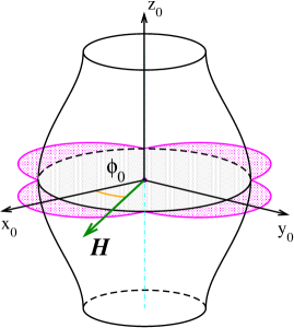
Figure 1: (Color online) In this paper we present calculations for a simple cylindrical Fermi surface and a Fermi surface shown here. The $d$-wave order parameter has lines of vertical nodes. Our goal is a calculation of the thermodynamic properties, such as specific heat and entropy, and their anisotropy under magnetic field rotations, $\phi_{0}$, in the $ab$-plane.

As one of our goals is the comparison of the results with the data on layered CeCoIn₅, Sec. IV.3 is devoted to the fully self-consistent calculations for more realistic quasi-cylindrical Fermi surfaces, Fig. 1. The discussion of the results, comparison with the data, and implications for future experiments are contained in Sec. V. The companion paper II uses these results to derive and discuss the behavior of the thermal conductivity.

We aimed to make the article useful to both theorists and experimentalists. Sec. IV.2 and Sec. V are probably most useful for those readers who are interested only in the overall physical picture and the behavior of the measured properties; the figures in Sec. IV.3 show the main differences between the self-consistent and non-self-consistent calculations.

II Quasiclassical Approach

II.1 Basic equations and formulation

We begin by writing down the quasiclassical equations for a singlet superconductor in magnetic field Eilenberger (1968); Larkin and Ovchinnikov (1969); Serene and Rainer (1983); Alexander et al. (1985); Houghton and Vekhter (1998); Eschrig et al. (1999) and summarizing the details relevant for our discussion. The equations are for the quasiclassical (low-energy $\varepsilon$) Green’s function, which is a matrix in the Nambu (spin and particle-hole) space,

$$\widehat{g}({\bf R},\hat{{\bf p}};\varepsilon)=\left(\begin{array}[]{cc}g&i\sigma_{2}f\\ i\sigma_{2}\underline{f}&-g\end{array}\right)\,.$$ (1)

This matrix propagator has been integrated over the quasiparticle band energy, and therefore depends only on the direction at the Fermi surface, $\hat{{\bf p}}$, and the center of mass coordinate, ${\bf R}$.

We formulate our approach in terms of the real-energy retarded, advanced, and Keldysh propagators. This is a natural path for the self-consistent calculation of the quasiparticle spectrum, needed for determination of thermodynamic properties such as entropy and heat capacity. Moreover, the Keldysh technique is the most direct route towards non-equilibrium calculations, required for the transport properties such as thermal conductivity, which is covered in the companion paper II. Consequently we establish a unified approach to describe both the thermodynamics and transport in the vortex state.

Retarded (R) and advanced (A) functions $\widehat{g}=\widehat{g}^{R,A}$ satisfy (we take the electron charge $e<0$)

$$[(\varepsilon+{e\over c}{\bf v}_{f}(\hat{{\bf p}}){\bf A}({\bf R}))\,\widehat{\tau}_{3}-\widehat{\Delta}({\bf R},\hat{{\bf p}})-\widehat{\sigma}_{imp}({\bf R};\varepsilon),$$

$$\widehat{g}({\bf R},\hat{{\bf p}};\varepsilon)]+i{\bf v}_{f}(\hat{{\bf p}})\cdot\mbox{\boldmath$\nabla_{\mbox{\tiny${\bf R}$}}$}\;\widehat{g}({\bf R},\hat{{\bf p}};\varepsilon)=0\,,$$ (2)

together with the normalization condition

$$\widehat{g}^{R,A}({\bf R},\hat{{\bf p}};\varepsilon_{m})^{2}=-\pi^{2}\widehat{1}\,.$$ (3)

Here $\varepsilon$ is the real frequency, ${\bf v}_{f}(\hat{{\bf p}})$ is the Fermi velocity at a point $\hat{{\bf p}}$ on the FS. The magnetic field is described by the vector potential ${\bf A}({\bf R})$, and the self-energy $\widehat{\sigma}$ is due to impurity scattering. The equations for the retarded and the advanced functions differ in the definition of the corresponding self-energies.

The mean field order parameter,

$$\widehat{\Delta}=\left(\begin{array}[]{cc}0&i\sigma_{2}\Delta\\ i\sigma_{2}\Delta^{*}&0\end{array}\right)\,,$$ (4)

is defined via the self-consistency equation involving the Keldysh function $f^{K}$,

$$\Delta({\bf R},\hat{{\bf p}})=\int{d\varepsilon\over 4\pi i}\int d\hat{{\bf p}}^{\prime}_{\mbox{\tiny FS}}\;n_{f}(\hat{{\bf p}}^{\prime})\,V(\hat{{\bf p}},\hat{{\bf p}}^{\prime})\,f^{K}({\bf R},\hat{{\bf p}}^{\prime};\varepsilon)\,,$$ (5)

In equilibrium $f^{K}=(f^{R}-f^{A})\tanh(\varepsilon/2T)$, and we obtain the usual self-consistency equation computing the $\varepsilon$-integral in the upper (lower) half-plane for $f^{R}~{}(f^{A})$.

We wrote Eq.(5) for a general Fermi surface, and therefore introduced the density of states (DOS) at a point $\hat{{\bf p}}$ on the Fermi surface in the normal state, $N_{f}(\hat{{\bf p}})$. The net density of states, ${\cal N}_{f}=\int d\hat{{\bf p}}_{\mbox{\tiny FS}}N_{f}(\hat{{\bf p}})$, and we define $n_{f}(\hat{{\bf p}})=N_{f}(\hat{{\bf p}})/{\cal N}_{f}$. We absorbed the net DOS, ${\cal N}_{f}$, into the definition of the pairing potential, $V(\hat{{\bf p}},\hat{{\bf p}}^{\prime})$.

Since below we frequently perform the integrals over the Fermi surface, we introduce a shorthand notation

$$\langle\;\bullet\;\rangle_{\mbox{\tiny FS}}=\int d\hat{{\bf p}}_{\mbox{\tiny FS}}\;n_{f}(\hat{{\bf p}})\;\bullet\,,$$ (6)

so that the the gap equation above can be rewritten as

$$\Delta({\bf R},\hat{{\bf p}})=\int{d\varepsilon\over 4\pi i}\,\langle\,V(\hat{{\bf p}},\hat{{\bf p}}^{\prime})\,f^{K}({\bf R},\hat{{\bf p}}^{\prime};\varepsilon)\rangle_{\mbox{\tiny FS}}\,.$$ (7)

All calculations below are for separable pairing,

$$V(\hat{{\bf p}},\hat{{\bf p}}^{\prime})=V_{s}\,{\cal Y}(\hat{{\bf p}})\,{\cal Y}(\hat{{\bf p}}^{\prime})\,,$$ (8)

where ${\cal Y}(\hat{{\bf p}})$ is the normalized basis function for the particular angular momentum, $\langle{\cal Y}(\hat{{\bf p}})^{2}\rangle_{{\mbox{\tiny FS}}}=1$. For example, for $d_{x^{2}-y^{2}}$ gap over a Fermi surface parameterized by angle $\phi$, we have ${\cal Y}(\phi)=\sqrt{2}\cos 2\phi$. Hence the order parameter is $\Delta({\bf R},\hat{{\bf p}})=\Delta({\bf R}){\cal Y}(\hat{{\bf p}})$.

Finally, we include the isotropic impurity scattering via the self-energy,

$$\widehat{\sigma}_{imp}({\bf R};\varepsilon)=\left(\begin{array}[]{cc}D+\Sigma&i\sigma_{2}\Delta_{imp}\\ i\sigma_{2}\underline{\Delta}_{imp}&D-\Sigma\end{array}\right)=n_{imp}\hat{t}({\bf R};\varepsilon)\,.$$ (9)

Here $n_{imp}$ is the impurity concentration, and, in the self-consistent $t$-matrix approximation,

$$\hat{t}({\bf R};\varepsilon)=u\hat{1}+u{\cal N}_{f}\langle\widehat{g}({\bf R},\hat{{\bf p}};\varepsilon)\rangle_{\mbox{\tiny FS}}\;\hat{t}({\bf R};\varepsilon)\,,$$ (10)

where $u$ is the single impurity isotropic potential. Comparing Eq. (2) and Eq. (9) we see that $\Sigma$ effectively renormalizes the energy $\varepsilon$, while $\Delta_{imp}$ accounts for the impurity scattering in the off-diagonal channel. The term $D\,\widehat{1}$ drops out of equations for the retarded and advanced Green’s functions since the unit matrix commutes with the Green’s function in Eq. (2). This term, however, generally appears in the Keldysh part, and has a substantial effect on transport properties. Hirschfeld et al. (1988); Löfwander and Fogelström (2004) Below we parameterize the scattering by the “bare” scattering rate, $\Gamma=n_{imp}/\pi{\cal N}_{f}$, and the phase shift $\delta_{0}$ of the impurity scattering, $\tan\delta_{0}=\pi u{\cal N}_{f}$.

In equilibrium we explicitly write Eqs. (2)-(3) as a system of equations,

$$g^{2}-f\,\underline{f}=-\pi^{2}\,,$$ (11a)

$$i{\bf v}_{f}(\hat{{\bf p}})\cdot\mbox{\boldmath$\nabla_{\mbox{\tiny${\bf R}$}}$}\;g+\widetilde{\Delta}\underline{f}-\widetilde{\underline{\Delta}}f=0\,,$$ (11b)

$$\left[-2i\tilde{\varepsilon}+{\bf v}_{f}(\hat{{\bf p}})\left(\mbox{\boldmath$\nabla_{\mbox{\tiny${\bf R}$}}$}-\frac{2ie}{c}{\bf A}({\bf R})\right)\right]f=2i\widetilde{\Delta}g\,,$$ (11c)

$$\left[-2i\tilde{\varepsilon}-{\bf v}_{f}(\hat{{\bf p}})\left(\mbox{\boldmath$\nabla_{\mbox{\tiny${\bf R}$}}$}+\frac{2ie}{c}{\bf A}({\bf R})\right)\right]\underline{f}=2i\underline{\widetilde{\Delta}}g\,,$$ (11d)

where $\tilde{\varepsilon}=\varepsilon-\Sigma$, $\widetilde{\Delta}=\Delta+\Delta_{imp}$, and $\widetilde{\underline{\Delta}}=\Delta^{*}+\underline{\Delta}_{imp}$.

II.2 Vortex state ansatz and Brandt-Pesch-Tewordt approximation

So far our discussion remained completely general. In the vortex state of a superconductor, the order parameter and the field vary in space, and the quasiclassical equations have to be solved together with the self-consistency equations for the gap function, and Maxwell’s equation for the self-consistently determined magnetic field and the vector potential. Finding a general non-uniform solution of such a system is a daunting, or even altogether impossible, task. Therefore we make several simplifying assumptions and approximations that allow us to obtain a closed form solution for the Green’s function.

First, we assume the magnetic field to be uniform. This assumption is valid for fields $H\gg H_{c1}$, where the typical intervortex spacing (of the order of the magnetic length, $\Lambda=(\hbar c/2|e|B)^{1/2}$) is much smaller than the penetration depth, the diamagnetic magnetization due to the vortices is negligible compared to the applied field, and the local field is close to the applied external field, $B\approx H$. All the materials for which the anisotropy measurements have been performed are extreme type-II superconductors, where this assumption is valid over essentially the entire field range below $H_{c2}$.

In writing the quasiclassical equations we only included the orbital coupling to the magnetic field, assuming that it dominates over the the paramagnetic (Zeeman) contribution. This is valid for most superconductors of interest, and the detailed analysis of the Zeeman splitting will be presented separately  Vorontsov and Vekhter (2006-7);the main conclusions of this paper remain unaffected.

Second, we take an Abrikosov-like vortex lattice ansatz for the spatial variation of the order parameter, which is a linear superposition of the single-vortex solutions in the plane normal to the field. We enforce the self-consistency condition, which requires going beyond the simple form suggested by the linearized Ginzburg-Landau equations. The details of this choice are given in Sec.III below.

In the vortex lattice state the quasiclassical equations generally do not allow solution in a closed form. We therefore employ a variant of the approximation originally due to Brandt, Pesch and Tewordt (BPT) Brandt et al. (1967). The method consists of replacing the diagonal part of the Green’s function by its spatial average, while keeping the full spatial structure of the off-diagonal terms. It was initially developed to describe superconductors near the upper critical field, where the amplitude of the order parameter is suppressed throughout the bulk, and the approximation is nearly exact. This is confirmed by expanding the Green’s function in the the Fourier components of the reciprocal vortex lattice, $g({\bf R},\hat{{\bf p}};\varepsilon)=\sum_{\bf K}\;g({\bf K},\hat{{\bf p}};\varepsilon)\exp(i{\bf K}{\bf R})$. and noticing that $g^{R}({\bf K})\propto\exp(-\Lambda^{2}{{\bf K}}^{2})$ so that the ${\bf K}=0$ component is exponentially dominant.Brandt et al. (1967) In situations where the states inside vortex cores are not crucial for the analysis, such as in extreme type-II ,Brandt (1976) or nodal superconductors Won and Maki (1996); Vekhter and Houghton (1999) the method remains valid essentially over the entire field range. Consequently the BPT approach and its variations was extensively used to study unconventional superconductors in the vortex state.Vekhter and Houghton (1999); Kusunose (2004); Tewordt and Fay (2005) One of the advantages of the method that it reproduces correctly the $H=0$ BCS limit,Houghton and Vekhter (1998) and therefore may be used to interpolate over all fields. One, however, needs to be cautious in computing the properties of impure systems: averaging over the intervortex distance ($\sim\Lambda$) prior to averaging over impurities is allowed only when $\Lambda/\ell\ll 1$, where $\ell$ is the mean free path, and hence the approach does break down at very low fields, and only asymptotically approaches the zero field result. We show the signatures of this breakdown in Sec. IV.3.

The use of the BPT approximation relaxes the constraints imposed by the assumption of a perfectly periodic vortex arrangement. Indeed, averaging over the unit cell of the vortex lattice is somewhat akin to the coherent potential approximation in many body physics, although with an important caveat that this is only done for the normal part of the matrix Green’s function. Consequently, the results derived within this approach are also applicable to moderately disordered vortex solids.

III Single-particle Green’s function

Hereafter we use $g$ to denote the spatially averaged electron Green’s function, $g\equiv g(\hat{{\bf p}};\varepsilon)=\overline{g({\bf R},\hat{{\bf p}};\varepsilon)}$. The approach we take here follows the standard practice Pesch (1975); Houghton and Vekhter (1998); Vekhter and Houghton (1999); Kusunose (2004) of determining $g$ from the spatially averaged normalization condition, Eq.(11a),

$$g^{2}-\overline{\underline{f}\,f}=-\pi^{2}\,.$$ (12)

Here we defined the average over vortex lattice of a product as

$$\overline{f_{1}\,f_{2}}=\int{d{\bf R}\over V}\,f_{1}({\bf R})f_{2}({\bf R})\,.$$ (13)

The anomalous components of the Green’s function satisfy Eqs.(11c)-(11d). Formally, the solution is obtained by acting with the inverse of the differential operator in the right hand side on the product $\widetilde{\Delta}\,g$ and $\underline{\widetilde{\Delta}}\,g$ respectively. Upon replacement of $g$ by its average, the operator acts solely on the order parameter,

$$f({\bf R},\hat{{\bf p}};\varepsilon)= 2ig(\hat{{\bf p}};\varepsilon)\;\hat{O}_{f}\,\widetilde{\Delta}({\bf R},\hat{{\bf p}};\varepsilon)$$ (14a)

$$\underline{f}({\bf R},\hat{{\bf p}};\varepsilon)= 2ig(\hat{{\bf p}};\varepsilon)\;\hat{O}_{\underline{f}}^{*}\,\widetilde{\underline{\Delta}}({\bf R},\hat{{\bf p}};\varepsilon)\,,$$ (14b)

where

$$\hat{O}_{f} = [-2i\tilde{\varepsilon}+{\bf v}_{f}(\hat{{\bf p}})\,(\mbox{\boldmath$\nabla_{\mbox{\tiny${\bf R}$}}$}-i{2e\over c}{\bf A}({\bf R}))]^{-1}\,,$$ (15a)

$$\hat{O}_{\underline{f}}^{*} = [-2i\tilde{\varepsilon}-{\bf v}_{f}(\hat{{\bf p}})\,(\mbox{\boldmath$\nabla_{\mbox{\tiny${\bf R}$}}$}+i{2e\over c}{\bf A}({\bf R}))]^{-1}\,.$$ (15b)

The strategy is to use a vortex lattice solution as an input, compute the anomalous Green’s functions $f$ and $\underline{f}$ in terms of $g$ from Eq.(14), determine $g$ from the normalization condition, and then enforce the self-consistency on $\Delta$ and the impurity self-energies. In principle, any complete set of basis functions is suitable for expanding both $\Delta(\bm{R},\hat{\bf p})$ and $f(\bm{R},\hat{\bf p})$. In practice, of course, we are looking for an expansion that can be truncated after very few terms, enabling efficient computation of the functions. The Abrikosov lattice ansatz for $\Delta(\bm{R})$ is a superposition of the functions corresponding to the single vortex solution of the Ginzburg-Landau equations, and therefore it is natural to use these functions as our basis.

For an $s$-wave superconductor with an axisymmetric Fermi surface (isotropic in the plane normal to the field), it is well known that the vortex lattice is given by a superposition of the single flux line solutions, the oscillator (Landau level, or LL) functions, $\Phi_{0}(x-x_{0})$, centered at different points in the plane normal to the applied field Tinkham (1985)

$$\Delta(\bm{R})=\sum_{k_{y}}C_{k_{y}}e^{ik_{y}y}\Phi_{0}\left({x-\Lambda^{2}k_{y}\over\Lambda}\right)\,.$$ (16)

Here the symmetry of the coefficients $C_{k_{y}}$ determines the structure of the lattice. This form emerges from the solution of the linearized Ginzburg-Landau (GL), and is also consistent with the solution of the linearized, with $g=-i\pi$, quasiclassical equations. Moreover, this form is valid down to low fields as the admixture of the contributions from higher Landau levels, $\Phi_{n}$ with $n\neq 0$, to $\Delta(\bm{R})$ remains negligible.Li and Rosenstein (1999) Consequently, the set of oscillator functions, $\Phi_{n}$, provides a convenient basis for the expansion of anomalous functions $f$. It is common to rewrite the operator $\hat{O}$ via the bosonic creation and annihilation operators, $a^{\dagger}$ and $a$. Houghton and Vekhter (1998) At the microscopic level, inserting this ansatz for $\Delta(\bm{R})$ into the quasiclassical equations, Eqs.(14), and enforcing the self-consistency condition, yields the order parameter which only includes the ground state oscillator functions, justifying use of Eq. (16) Houghton and Vekhter (1998).

In unconventional superconductors the situation is more complex. While the solution of the GL equations are still given by Eq. (16), this form is not a self-consistent solution of the linearized microscopic equations: the momentum and the real space dependence of the order parameter are coupled via the action of the operator ${\bf v}_{f}(\hat{{\bf p}})\cdot\mbox{\boldmath$\nabla_{\mbox{\tiny${\bf R}$}}$}$. Since the wave functions for Landau levels form a complete set, they can still be used as a basis for the expansion. The microscopic equations mix different Landau levels, and the self-consistent solution for the vortex state involves a linear combination of an infinite number of $\Phi_{n}$ at each site Luk’yanchuk and Mineev (1987). For the axisymmetric case the spatial structure of $\Delta(\bm{R})$ is still close to that for the $s$-wave case, and the weight of the higher Landau levels in the self-consistent solution decreases rapidly with increasing $n$ Luk’yanchuk and Mineev (1987); Won and Maki (1996). Hence in practice the series in $n$ is truncated either at $n=0$ (as for $s$-wave) or at the second non-vanishing term Won and Maki (1996); Vekhter and Houghton (1999). While this is often sufficient to describe the salient features of the thermal and transport coefficients, care should be taken in determining the anisotropies of these coefficients under a rotated field: the anisotropy is often of the order of a percent, and the structure of the vortex lattice should therefore be determined to high accuracy as well.

The situation is even more complex for unconventional superconductors with non-spherical Fermi surface, when the Fermi velocity is anisotropic in the plane normal to the applied field. Quasi-two dimensional systems with the field in the plane, such as shown in Fig. 1, give one example of such difficulties. Frequently in the microscopic theory the expansion is still carried out in the LL functions using the operators for the isotropic case. These functions are now strongly mixed, and hence (numerically intensive) inclusion of many LL is required before the self-consistency is reached. Determining magnetization in the vortex state, for example, was carried out with 6 LL functions Adachi et al. (2005).

This difficulty, however, is largely self-inflicted since, in contrast to the isotropic case, the LL functions in the form used in Ref. Adachi et al., 2005 are not the solutions to the linearized GL equations. For an arbitrary Fermi surface the coefficients of the Ginzburg-Landau expansion are anisotropic, and the vortex lattice solution is given by the $n=0$ Landau Level in the rescaled, according to the anisotropy, coordinates. Ketterson and Song (1999) We show in Appendix A that the proper rescaling is

$$x^{\prime}=x/\sqrt{S_{f}},\qquad y^{\prime}=y\sqrt{S_{f}}\,,$$ (17)

where $S_{f}$ is a measure of the anisotropy of the Fermi surface. For a FS with rotational symmetry around the axis $z_{0}$, and for the field at an angle $\theta_{H}$ to this axis,

$$S_{f}=\sqrt{\cos^{2}\theta_{H}+{v_{0||}^{2}\over v_{0\perp}^{2}}\sin^{2}\theta_{H}}\,.$$ (18)

Here $v_{0\perp}^{2}=2\langle{\cal Y}^{2}(\hat{{\bf p}})v^{2}_{\perp i}(p_{z})\rangle_{\mbox{\tiny FS}}$ and $v_{0\parallel}^{2}=2\langle{\cal Y}^{2}(\hat{{\bf p}})v^{2}_{\parallel}(p_{z})\rangle_{\mbox{\tiny FS}}$, where $v_{\parallel}$ is the projection of the Fermi velocity on the $z_{0}$ axis, and $v_{\perp i}$ with $i=x_{0},y_{0}$ is the projection on the axes in the plane normal to $z_{0}$. For the field in the basal plane $\theta_{H}=\pi/2$, and therefore $S_{f}=v_{0||}/v_{0\perp}$.

The appropriate basis functions, which we use hereafter, correspond to the oscillator states in the rescaled coordinates. If we chose the direction of the field as the $z$-axis,

$$\widetilde{\Phi}_{n}(x,k_{y})=\Phi_{n}\left({x-\Lambda^{2}\sqrt{S_{f}}k_{y}\over\Lambda\sqrt{S_{f}}}\right)\,.$$ (19)

For an $s$-wave superconductor the $n=0$ ansatz for $\Delta(\bm{R})$ satisfies microscopic equations, while for unconventional order parameters different LLs are once again mixed. However, with our choice of the basis functions this mixing is weak, enabling us to truncate the expansion at three components. Consequently, we use a generalized form of the vortex lattice $\Delta(\bm{R},\hat{{\bf p}})=\Delta(\bm{R}){\cal Y}(\hat{{\bf p}})$, where

$$\Delta(\bm{R})=\sum_{n}\Delta_{n}\mbox{$\displaystyle\langle\,{\bf R}\,|\,n\,\rangle$}$$ (20a)

$$\mbox{$\displaystyle\langle\,{\bf R}\,|\,n\,\rangle$}=\sum_{k_{y}}C_{k_{y}}^{(n)}{e^{ik_{y}\sqrt{S_{f}}y}\over\sqrt[4]{S_{f}\Lambda^{2}}}\widetilde{\Phi}_{n}\left(x,k_{y}\right)\,.$$ (20b)

The normalizing factor in Eq.(20b) is introduced so that the states $\displaystyle\langle\,{\bf R}\,|\,n\,\rangle$ are orthonormal, i.e.

$$\int\frac{d{\bm{R}}}{V}\mbox{$\displaystyle\langle\,{\bf R}\,|\,n\,\rangle$}[\mbox{$\displaystyle\langle\,{\bf R}\,|\,n^{\prime}\,\rangle$}]^{*}=\delta_{n,n^{\prime}}\,,$$ (21)

provided

$$\sum_{k_{y}}|C_{k_{y}}^{(n)}|^{2}=1.$$ (22)

Consequently $\Delta_{n}$ in Eq.(20a) has the meaning of the amplitude of the appropriate component of the order parameter in the LL expansion.

The ladder operators,

$$a={\Lambda\over\sqrt{2}}\left(-\mbox{\boldmath$\nabla$}_{x^{\prime}}+i(\mbox{\boldmath$\nabla$}_{y^{\prime}}+i{x^{\prime}\over\Lambda^{2}})\right)\,,$$ (23a)

$$a^{\dagger}={\Lambda\over\sqrt{2}}\left(\mbox{\boldmath$\nabla$}_{x^{\prime}}+i(\mbox{\boldmath$\nabla$}_{y^{\prime}}+i{x^{\prime}\over\Lambda^{2}})\right)\,,$$ (23b)

obey the usual bosonic commutation relations, $[a,a^{\dagger}]=1$, $[a,a]=[a^{\dagger},a^{\dagger}]=0$, and connect the states $|n\rangle$ via $a\mbox{$\displaystyle|\,n\,\rangle$}=\sqrt{n}\mbox{$\displaystyle|\,n-1\,\rangle$}$ and $a^{\dagger}\mbox{$\displaystyle|\,n\,\rangle$}=\sqrt{n+1}\mbox{$\displaystyle|\,n+1\,\rangle$}$.

To solve Eq.(14) we rewrite the differential operators $O_{f}$ and $O_{\underline{f}}$ via the ladder operators, Eq.(23), and find

$$O_{f} = [-2i\tilde{\varepsilon}+{\bf v}_{f}(\hat{{\bf p}})\,(\mbox{\boldmath$\nabla_{\mbox{\tiny${\bf R}$}}$}-i{2e\over c}{\bf A}({\bf R}))]^{-1}$$ (24)

$$= \left[-2i\tilde{\varepsilon}+\frac{1}{\sqrt{2}\Lambda}\,\left(v_{-}(\hat{{\bf p}})a^{\dagger}-v_{+}(\hat{{\bf p}})a\right)\right]^{-1},$$ (25)

where

$$v_{\pm}=v_{x}(\hat{{\bf p}})/\sqrt{S_{f}}\pm iv_{y}(\hat{{\bf p}})\sqrt{S_{f}}$$ (26)

For convenience we introduce the rescaled Fermi velocity

$$\tilde{v}_{f}(\hat{{\bf p}})_{x}=v_{f}(\hat{{\bf p}})_{x}/\sqrt{S_{f}}\quad,\quad\tilde{v}_{f}(\hat{{\bf p}})_{y}=v_{f}(\hat{{\bf p}})_{y}\sqrt{S_{f}}\,,$$ (27)

and its projection on the $xy$-plane (perpendicular to H),

$$|\tilde{v}_{f}^{\perp}(\hat{{\bf p}})|=\sqrt{\tilde{v}_{f}(\hat{{\bf p}})_{x}^{2}+\tilde{v}_{f}(\hat{{\bf p}})_{y}^{2}}\,,$$ (28)

as well as the “phase factors”,

$$\tilde{v}_{\pm}(\hat{{\bf p}})=\frac{\tilde{v}_{f}(\hat{{\bf p}})_{x}\pm i\tilde{v}_{f}(\hat{{\bf p}})_{y}}{|\tilde{v}_{f}^{\perp}|}\,.$$ (29)

The off-diagonal parts of the matrix Green’s function can be expressed in terms of the normal component $g$, and written as a series over the set $\displaystyle\langle\,{\bf R}\,|\,m\,\rangle$. The solution is based on exponentiating the operator $O_{f}$ to explicitly evaluate the result of its action on the order parameter Pesch (1975); Houghton and Vekhter (1998), and is detailed in Appendix B. We find

$$f({\bf R},\hat{{\bf p}};\varepsilon)=\sum_{m}f_{m}(\hat{{\bf p}},\varepsilon)\mbox{$\displaystyle\langle\,{\bf R}\,|\,m\,\rangle$}\,,$$ (30a)

$$f_{m}(\hat{{\bf p}},\varepsilon)=ig\,\sum_{n}(-\tilde{v}_{-}(\hat{{\bf p}}))^{m-n}\,{\cal D}_{m,n}(\varepsilon,|\hat{{\bf p}}|)\widetilde{\Delta}_{n}(\hat{{\bf p}};\varepsilon)\,,$$ (30b)

where $\widetilde{\Delta}_{n}(\hat{{\bf p}};\varepsilon)=\Delta_{n}(\hat{{\bf p}})+\Delta_{imp,n}(\varepsilon)$. The coefficients

$${\cal D}_{m,n}(\varepsilon,|\hat{{\bf p}}|)=\sqrt{\pi}{2\Lambda\over|\tilde{v}^{\perp}_{f}|}\sum_{j=0}^{min(m,n)}(-1)^{n_{1}}D_{m,n}^{n_{1},n_{2}}\left({2\tilde{\varepsilon}\Lambda\over|\tilde{v}^{\perp}_{f}|}\right)\,,$$ (31)

with $n_{1}(j)=j+(|m-n|-(m-n))/2$, $n_{2}(j)=j+(|m-n|+(m-n))/2$ in each term and

$$D^{n_{1},n_{2}}_{m,n}(z)=\left({-i\over\sqrt{2}}\right)^{n_{1}+n_{2}}{\sqrt{n!}\sqrt{m!}\over(n-n_{1})!n_{1}!n_{2}!}W^{(n_{1}+n_{2})}(z)\,,$$ (32)

where $W^{(n)}(z)$ is the $n$-th derivative of the function $W(z)=\exp(-z^{2})\mbox{erfc}(-iz)$. These functions have the following symmetries: $W^{(n)}(z)^{*}=(-1)^{n}W^{(n)}(-z^{*})$, ${\cal D}_{m,n}=(-1)^{m-n}{\cal D}_{n,m}$ and $D^{n_{1},n_{2}}_{m,n}(z)^{*}=D^{n_{1},n_{2}}_{m,n}(-z^{*})$.

The diagonal part, $g$, is determined from the average $\underline{f}f$ and the normalization condition. The details, once again, are relegated to Appendix B, with the result

$$g = -i\pi/\sqrt{1+P}\,,$$ (33a)

$$P = -i\sqrt{\pi}{2\over w^{2}}\sum_{n}\sum_{m}\widetilde{\underline{\Delta}}_{n}\widetilde{\Delta}_{m}\sum^{\prime}_{k,l\geq 0}\frac{(\tilde{v}_{+})^{l}(-\tilde{v}_{-})^{k}}{l!\,k!}$$ (33b)

$$\times\mbox{$\displaystyle\langle\,n\,|$}a^{{\dagger}k}a^{l}\mbox{$\displaystyle|\,m\,\rangle$}\left({-i\over\sqrt{2}}\right)^{k+l}W^{(k+l+1)}\left({\sqrt{2}\tilde{\varepsilon}\over w}\right)\,,$$

where $w=|\tilde{v}^{\perp}_{f}|/\sqrt{2}\Lambda$, and the prime over the $k,l$-sum denotes the restriction that the matrix element $\mbox{$\displaystyle\langle\,n\,|$}a^{{\dagger}k}a^{l}\mbox{$\displaystyle|\,m\,\rangle$}=\sqrt{n!m!/(n-k)!(m-l)!}$ is non-zero only for $k\leq n$, $l\leq m$ and $k-l=n-m$.

If we truncate the expansion of the order parameter in the vortex state at the lowest Landau level function, $n=0$, we find from Eqs.(33)

$$g=\frac{-i\pi}{\sqrt{1-i\sqrt{\pi}\left(\frac{2\Lambda}{|\tilde{v}_{f}^{\perp}|}\right)^{2}\,W^{\prime}(\frac{2\tilde{\varepsilon}\Lambda}{|\tilde{v}_{f}^{\perp}|})\,\widetilde{\Delta}_{0}\underline{\widetilde{\Delta}}_{0}}}\,,$$ (34)

which agrees with previously obtained expressionsPesch (1975); Klimesch and Pesch (1978); Houghton and Vekhter (1998); Vekhter and Houghton (1999); Kusunose (2004). In the zero field limit, $\Lambda\propto 1/\sqrt{H}\to\infty$, we use the asymptotic behavior at large values of the argument, $W(z)\approx i/\sqrt{\pi}z$, $W^{\prime}(z)\approx-i/(\sqrt{\pi}z^{2})$, to verify that this Green’s function tends to the BCS limit Houghton and Vekhter (1998); Vekhter and Houghton (1999), and therefore all the conventional results for the density of states in nodal superconductors immediately follow.

Eqs.(30b) and (33) give the solution of the quasiclassical equations in the BPT approximation for a given vortex lattice and impurity self-energies, i.e. provided the coefficients $\Delta_{n},\underline{\Delta}_{m}$ and $\Sigma,\Delta_{imp,n},\underline{\Delta}_{imp,m}$ are known. The self-consistency equations for these coefficients,

$$\Delta_{n}\ln{T\over T_{c0}}=\int{d\varepsilon\over 4\pi i}\int d\hat{{\bf p}}_{\mbox{\tiny FS}}\;n_{f}(\hat{{\bf p}})\,{\cal Y}(\hat{{\bf p}})\,\times$$ (35)

$$\times\left(f^{R}_{n}(\hat{{\bf p}};\varepsilon)-\underline{f}^{R}_{n}(\hat{{\bf p}};\varepsilon)^{*}-2\pi i{\Delta_{n}{\cal Y}(\hat{{\bf p}})\over\varepsilon}\right)\tanh{\varepsilon\over 2T}\,,$$

and the equations for the impurity retarded and advanced self-energy, Eq. (9), written explicitly through solution of Eq. (10) for the $t$-matrix,

$$\widehat{t}=\left(\begin{array}[]{cc}t_{+}+t_{-}&t_{\Delta}\,i\sigma_{2}\\ i\sigma_{2}\,\underline{t}_{\Delta}&t_{+}-t_{-}\end{array}\right)={1\over n_{imp}}\frac{\Gamma\sin^{2}\delta_{0}}{1-{\sin^{2}\delta_{0}\over\pi^{2}}(\langle g\rangle^{2}-\overline{\langle f\rangle\langle\underline{f}\rangle}+\pi^{2})}\left(\begin{array}[]{cc}\cot\delta_{0}+\langle g\rangle/\pi&(\langle f\rangle/\pi)\,i\sigma_{2}\\ i\sigma_{2}\,(\langle\underline{f}\rangle/\pi)&\cot\delta_{0}-\langle g\rangle/\pi\end{array}\right)\,,$$ (36)

complete the closed form solution. Here $T_{c0}$ is the critical temperature for the clean system, $\Gamma=0$, which we used to eliminate the interaction strength, $V_{s}$, and the high energy cutoff. The elimination can also be done in favor of the impurity suppressed $T_{c}$, see e.g. Ref.Xu et al., 1995b.

IV Heat capacity

IV.1 Density of states and the specific heat

Once we self-consistently determined the Green’s function, we can calculate the quasiparticle spectrum. We use the standard definition for the angle-resolved density of states at the Fermi surface,

$$\frac{N(\varepsilon,\hat{{\bf p}})}{N_{f}(\hat{{\bf p}})}=-{1\over\pi}\mathfrak{Im}\,g^{R}(\hat{{\bf p}},\varepsilon)\,,$$ (37)

where $N_{f}$ is the normal state DOS.

The heat capacity is the derivative of the entropy, $C=T\,\partial S/\partial T$, where

$$S = -2\sum_{\bf k}[(1-f(E_{\bf k}))\ln(1-f(E_{\bf k}))+f(E_{\bf k})\ln f(E_{\bf k})]$$

$$= -2\int\limits_{-\infty}^{+\infty}d\varepsilon\,N(\varepsilon)\,[(1-f(\varepsilon))\ln(1-f(\varepsilon))+f(\varepsilon)\ln f(\varepsilon)]\,,$$

$f(\varepsilon)=1/(e^{\varepsilon/T}+1)$ is the Fermi function, and $N(\varepsilon)=\int d\hat{{\bf p}}\,N(\varepsilon,\hat{{\bf p}})$ is the net DOS at energy $\varepsilon$. In practice, numerical differentiation of the entropy is computationally either noisy or very time consuming due to high accuracy required in finding $S$, and therefore not very convenient. At low temperatures the order parameter and the density of states are weakly temperature dependent, and therefore the specific heat can be obtained by differentiating only the Fermi functions. This leads to the well-known expression

$$C(T,\bm{H})=\frac{1}{2}\int\limits^{+\infty}_{-\infty}\;d\varepsilon\;\frac{\varepsilon^{2}\;N(T,\bm{H};\varepsilon)}{T^{2}\cosh^{2}(\varepsilon/2T)}\,,$$ (38)

that lends itself more efficiently to numerical work. Note that the $x^{2}/\cosh^{2}(x/2)$ function has a single sharp peak at $x\sim 2.5$, so the DOS at $\varepsilon\sim 2.5\div 3\,T$ contributes the most to the $C/T$. The difference between the specific heat defined from the density of state and the exact result is, of course, dramatic near the phase transition from the normal metal to a superconductor, where the peak in the specific heat is entirely due to entropy change not accounted for in Eq. (38). At the same time, the regime where the anisotropy of $C(T,\bm{H})$ is measured is far from $T_{c}$, and there we find that the results are very weakly dependent on the method of calculation. We therefore use the approximate expression above except where noted, and give a more detailed account of the difference between the two approaches for the specific Fermi surface shape in Sec. IV.3.

IV.2 Cylindrical Fermi surface

We are now prepared to consider the behavior of the specific heat in the vortex state of a superconductor. As mentioned above, our goal is to analyze the variations of the specific heat when the applied field is rotated with respect to the nodal directions. We consider first the simplest model of a cylindrical Fermi surface with vertical lines of nodes, and the field applied in the basal plane, at varying angle to the crystal axes.

This is a simplified version of a model for layered compounds, such as CeCoIn₅, considered below in Sec. IV.3. There we compute the specific heat for a quasi-cylindrical Fermi surface, open and modulated along the $z_{0}$-axis. The main advantage of considering an uncorrugated cylinder first is that it provides a good basis for semi-analytical understanding of the main features of the thermodynamic properties. Moreover, this model gives results that are in semi-quantitative agreement with those for the more realistic model of Sec. IV.3.

The disadvantage of the model is that it is not self-consistent. If the Fermi surface is cylindrical, there is no component of the quasiparticle velocity along the $z_{0}$ direction (the axis of the cylinder). The field applied in the plane does not result in the Abrikosov vortex state, as the supercurrents cannot flow between the layers. Consequently, it is impossible to set up and solve the self-consistency equations for the order parameter as a function of the applied field. Nonetheless we assume the existence of the vortex lattice where the order parameter has a single $n=0$ Landau level component, with the amplitude $\Delta(T,H)=\Delta(T,0)\sqrt{1-H/H_{c2}(T)}$, analogous to Ref.Vekhter and Houghton, 1999; Vekhter et al., 1999. With this assumption, we solve self-consistently for the temperature-dependent $\Delta(T,0)$, and for the impurity self-energies. We consider the unitarity limit of impurity scattering (phase shift $\delta_{0}=\pi/2$). In the next section we compare this model with a more realistic fully self-consistent approach, and show that the major features of the two are very similar.

While in the cylindrical approximation the results depend solely on the ratio $H/H_{c2}$, for comparison with the results of the self-consistent calculation we recast them in similar form. We measure the field in the units of $B_{0}=\Phi_{0}/2\pi\xi_{0}^{2}$ where $\Phi_{0}=hc/2|e|$ is the flux quantum and $\xi_{0}=\hbar v_{f}/2\pi T_{c}$ is the temperature independent coherence length in the $ab$-plane. At zero temperature the upper critical field along the $c$-axis is computed self-consistently, $H_{c2,c}\approx 0.55B_{0}$. We set the in-plane $H_{c2}=1.1B_{0}$ to approximate the factor of 2 anisotropy found in CeCoIn₅, and choose the normal state scattering rate $\Gamma/2\pi T_{c}=0.007$ (suppression of the critical temperature $(T_{c0}-T_{c})/T_{c0}\approx 5\%$). We checked that the resulting map of the anisotropy in the specific heat in the $T$-$H$ plane does not strongly depend on this particular choice. Of course, large impurity scattering smears the angular variations.

For a single Landau level component the solutions for the Green’s function have a particularly simple form of Eq. (34). For a $d_{x^{2}-y^{2}}$ superconductor the gap function is $\Delta(\phi)=\Delta\cos 2\phi$. If the magnetic field is applied at an angle $\phi_{0}$ to the $x$-axis (inset in Fig. 2), the component of the Fermi velocity normal to the field is

$$v_{f}^{\perp}(\phi)=v_{f}\sin(\phi-\phi_{0}).$$ (39)

Therefore the Green’s function of Eq.(34) takes the form

$$g(\varepsilon,\phi)=\frac{-i\pi}{\sqrt{1-i\sqrt{\pi}\left(\frac{2\Lambda\Delta}{v_{f}|\sin(\phi-\phi_{0})|}\right)^{2}\,W^{\prime}(\frac{2\tilde{\varepsilon}\Lambda}{v_{f}|\sin(\phi-\phi_{0})|})\cos^{2}2\phi}}\,$$ (40)

Let us focus first on the residual density of states, $\varepsilon\rightarrow 0^{+}$ in the clean limit, $\Gamma=0$, to compare with the semiclassical Doppler approximation. In this case $W^{\prime}(0)=2i/\sqrt{\pi}$ and the density of states reduces to

$$N(0)=\int_{0}^{2\pi}{d\phi\over 2\pi}\frac{1}{\sqrt{1+{1\over 4z^{2}}{\cos^{2}2\phi\over\sin^{2}(\phi-\phi_{0})}}}$$ (41)

where $z=v_{f}/4\sqrt{2}\Lambda\Delta\sim\sqrt{H/H_{c2}}$. The DOS can be obtained analytically for the nodal and antinodal alignments of the field.

Node, $\phi_{0}=\pi/4$. Then Eq.(41) reduces to

$$N_{\mbox{\tiny node}}(0)={2\over\pi}{z\over\sqrt{1+z^{2}}}K\left({1\over\sqrt{1+z^{2}}}\right)\,,$$ (42)

where $K$ is the complete elliptic integral of the first kind. We use the convention of Ref. Gradshteyn and I.M.Ryzhik, 1980 for the argument of all elliptic functions. In the weak field limit, $z\ll 1$,

$$N_{\mbox{\tiny node}}(0)\simeq{2z\over\pi}\ln{4\over z}\,.$$ (43)

Antinode, $\phi_{0}=0$. The corresponding DOS is evaluated to be

$$N_{\mbox{\tiny antinode}}(0)={z\over(z^{2}+1/4)^{1/4}}{2\over\pi}\left[K(r)-{1\over 2}F(\alpha,r)\right]\,,$$ (44a)

where $$F(\alpha,r)$$ is the incomplete elliptic integral of the first kind, and

$$\alpha=\arccos\frac{1-\sqrt{z^{2}+1/4}}{1+\sqrt{z^{2}+1/4}}\;,\;r={1\over\sqrt{2}}\sqrt{1+{1+z^{2}\over\sqrt{1+4z^{2}}}}\,.$$ (44b)

At low fields, $z\ll 1$, the antinodal DOS

$$N_{\mbox{\tiny antinode}}(0)={2\sqrt{2}z\over\pi}\ln{4\sqrt{2}\over z}\,.$$ (45)

Apart from the logarithmic correction (which is rapidly washed away by finite impurity scattering), the antinodal DOS exceeds the nodal value by a factor $\sqrt{2}$, in complete agreement with the Doppler approach Vekhter et al. (1999). As the field increases however, Eqs. (42) and (44) predict a crossing point $z^{*}\sim 0.63$ above which the residual nodal DOS becomes greater than $N_{\mbox{\tiny antinode}}(0)$; this result was obtained numerically in Refs. Udagawa et al., 2004; Miranović et al., 2003. With our choice of $\Delta(H)=\Delta\sqrt{1-H/H_{c2}}$, the zero-temperature crossover point lies at $H^{*}/H_{c2}\sim 0.6$.

Similar analytic expressions cannot be written for finite energies and we evaluate the DOS and the specific heat numerically, including the impurity effects. Results for the anisotropy of the heat capacity are shown in Fig. 2. We present them in a form of a phase diagram (left panel) that shows the regions with the opposite anisotropy. Shaded (white) areas correspond to the minimum (maximum) of $C$ when ${\bf H}$ is along a node. Of course the node-antinode anisotropy disappears as the field $H\to 0$. Since we are primarily interested in comparison of our results with the experimental data, we focus on the regime of moderate fields, and show the evolution of specific heat for different directions of the field, $\phi_{0}$, with the temperature in the right panel of Fig. 2. Notice that at $\phi_{0}=45^{\circ}$, when the field is along a nodal direction, the minimum in $C(\phi_{0})$ evolves into the maximum as $T$ increases.

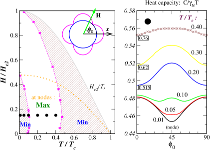
Figure 2: (Color online) Left panel: The phase diagram for the anisotropy of the heat capacity for cylindrical Fermi surface. At low $T$ and $H$ (shaded area) the minimum in the heat capacity occurs when the field point in a nodal direction, $\phi_{0}=45$. As $T$ increases the minimum first evolves into a maximum, and then switches back to a minimum. The inversion of zero energy DOS is indicated by the dotted line. Right panel: evolution of the heat capacity anisotropy with temperature for $H/H_{c2}=0.136$ (circles in the left panel). Some curves are shifted vertically for clarity, their original values at $\phi_{0}=0$ are shown in boxes. $\gamma_{N}$ is the Sommerfeld coefficient in the normal state.

Inversion of the anisotropy in the $T$-$H$ phase diagram is at odds with the semiclassical result that always predicts a minimum in the specific heat for the field parallel to the nodal direction. In the shaded area adjacent to the $H_{c2}(T)$ line in Fig. 2, with minima for ${\bf H}||\,node$, the specific heat is already sensitive to the density of states near the BCS singularity in the DOS at $\varepsilon\sim\Delta_{0}$, and therefore direct comparison with the semiclassical analysis is not possible. Moreover, we show in the following section that the self-consistent models require nodal-antinodal anisotropy of the upper critical field, and the results for this part of the phase diagram are modified.

On the other hand, the anisotropy inversion between the low-$T$, low-$H$ region, and the intermediate temperatures and fields, occurs still in the regime where the semiclassical logic may have been expected to work. The dotted line in the left panel of Fig. 2 separates the two regions of the residual zero-energy DOS: below that line $N_{\mbox{\tiny node}}(0)<N_{\mbox{\tiny antinode}}(0)$, while above the line $N_{\mbox{\tiny node}}(0)>N_{\mbox{\tiny antinode}}(0)$. The inversion of the anisotropy in the specific heat is clearly not just a consequence of the behavior of the zero-energy DOS found above. Recalling that $C/T$ is predominantly sensitive to the density of states at energies of the order of a few times $T$ (see Eq.(38)), we conclude that the origin of the anisotropy inversion is in the behavior of the finite energy DOS. We plot the low-energy $N(\varepsilon,{\bf H})$ at several values of the magnetic field in the left panel of Fig. 3. At low fields, the DOS anisotropy at small $\varepsilon$ agrees with the semiclassical prediction, but the density of states for the field along a node (dashed lines) and along an antinode (solid lines) become equal at a finite energy indicated by arrows. Above this energy the DOS anisotropy is reversed, and is manifested in the reversal of the specific heat anisotropy as $T$ increases. The crossing point moves to lower energies with increasing field, and is driven to zero when the residual, $\varepsilon=0$, DOS for the two directions become equal. In our numerical work with finite impurity scattering rate this occurs at $H^{*}\sim 0.5H_{c2}$, and we checked that $H^{*}\to 0.6H_{c2}$ as the system becomes more pure, in agreement with the analytical results above.

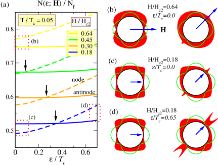
Figure 3: (Color online) Left: the low-energy part of the DOS for cylindrical FS. The nodal and antinodal DOS cross at finite energies (arrows). Right: the angle-resolved DOS (red shaded) for the two field orientations in the regions indicated by the dotted boxes in the left panel. The angle integrated DOS is given by the area of the shaded regions. See text for details.

As suggested by us in the short Letter communicating our main results, the inversion stems from the interplay between the energy shift and scattering due to magnetic field Vorontsov and Vekhter (2006). Magnetic field not only creates new quasiparticle states on the Fermi surface, but also scatters the quasiparticles and, consequently, re-distributes their spectral density. This scattering is present in the microscopic method, but not in the Doppler shift treatment. To understand this effect and to make connection with the semiclassical approach we analyze the angle-resolved DOS obtained from the Green’s function, Eq. (34). It is instructive to re-write the Green’s function in the BCS-like form which makes explicit the distinction between the energy shift and scattering rate. We define the “magnetic self-energy” $\Sigma=\Sigma^{\prime}-i\Sigma^{\prime\prime}$ from $(\varepsilon-\Sigma)^{-2}\equiv i\sqrt{\pi}(2\Lambda/|\tilde{v}_{f}^{\perp}|)^{2}\,W^{\prime}(2\tilde{\varepsilon}\Lambda/|\tilde{v}_{f}^{\perp}|)$ so that the Green’s function reads

$$g^{R}=-i\pi\left(1-\frac{|\Delta_{0}|^{2}{\cal Y}^{2}(\hat{\bf p})}{(\varepsilon-\Sigma^{\prime}(\varepsilon,{\bf H},\hat{{\bf p}})+i\Sigma^{\prime\prime}(\varepsilon,{\bf H},\hat{{\bf p}}))^{2}}\right)^{-1/2}\,.$$ (46)

The density of states for a given direction at the Fermi surface can be found from the comparison of $\varepsilon-\Sigma(\hat{{\bf p}})$ with $\Delta_{0}{\cal Y}(\hat{\bf p})=\Delta_{max}\cos 2\phi$. Since $W^{\prime}(x)$ is a complex-valued function, both $\Sigma^{\prime}$ and $\Sigma^{\prime\prime}$ are generally non-zero: the former shifts the quasiparticle energy, while the latter accounts for the direction-dependent scattering. For now we neglect the impurity broadening: for quasiparticles moving not too close to the field direction the field-induced scattering is normally greater than the scattering by impurities. Non-zero $\Sigma^{\prime\prime}$ is the key signature of our microscopic solution. Both real and imaginary components of the self-energy depend on the quasiparticle energy $\varepsilon$, the strength and direction of the field ${\bf H}$ and on the momentum of the quasiparticle with respect to both nodal direction and the field. Using the expansion around $W^{\prime}(0)=2i/\sqrt{\pi}$ at small values of the argument, and taking $W^{\prime}(z\gg 1)\approx-i/\sqrt{\pi}z^{2}$ for large arguments, we find two limiting cases,

$$\varepsilon-\Sigma\approx i{|\tilde{v}_{f}^{\perp}|\over 2\sqrt{2}\Lambda}+O\left(\frac{\Lambda^{2}\varepsilon^{2}}{|\tilde{v}_{f}^{\perp}|^{2}}\right),\;\mbox{if }\varepsilon\ll\frac{|\tilde{v}_{f}^{\perp}|}{2\Lambda}\;,$$ (47)

$$\varepsilon-\Sigma\approx\varepsilon+O\left(\frac{|\tilde{v}_{f}^{\perp}|^{2}}{\Lambda^{2}\varepsilon^{2}}\right),\qquad\;\;\;\mbox{if }\varepsilon\gg\frac{|\tilde{v}_{f}^{\perp}|}{2\Lambda}\,.$$ (48)

Note that $|\tilde{v}_{f}^{\perp}(\widehat{\bf p})|/2\Lambda\propto\sqrt{H}$ is the characteristic magnetic energy scale for quasiparticles at position $\widehat{\bf p}$ on the Fermi surface. In the first limit, valid at low energies (or moderately strong fields) for quasiparticle momenta away from the field direction, the imaginary part of the self-energy is dominant. In the opposite limit the effect of the field is small. Between these two limits, i.e. at finite energies, moderate fields and arbitrary $\hat{{\bf p}}$ , the real (energy shift) and the imaginary (scattering) parts of the self-energy can be comparable.

We can now analyse the angle-dependent contribution to the density of states from different regions at the Fermi surface at a given field, which is shown in the right panel of Fig. 3. Consider first very low energy $\varepsilon\to 0$, panels Fig. 3 b) and c), so that we are in the regime described by Eq.(47). At low fields, panel c), the characteristic energy, $|\tilde{v}_{f}^{\perp}(\widehat{\bf p})|/2\Lambda$ is smaller than the maximal gap, $\Delta_{max}$, and therefore most of the field-induced quasiparticle states appear near the nodes for which $|\tilde{v}_{f}^{\perp}(\widehat{\bf p})|$ is moderately large. Consequently, as in the semiclassical result, field applied along a nodal direction does not create quasiparticles near that node, while the field applied along the gap maximum generates new states at all nodes. The small contribution seen in the right frame of panel c) at the nodes aligned with the field is due to impurity scattering. Thus, while the scattering on the vortices, i.e. the imaginary part of Eq.(47), does produce a non-vanishing contribution to the DOS over most of the Fermi surface, at very low energy and low field the spectral weight of the field-induced states is mainly concentrated near the nodal points.

This changes as the field is increased, see panel b). At high field the Doppler shift and pairbreaking due to scattering are strong, and sufficient to contribute to the single particle DOS over almost the entire Fermi surface where $|\tilde{v}_{f}^{\perp}(\widehat{\bf p})|/2\Lambda\sim\Delta_{max}(H)$ (as a reminder, in our notations the maximal gap, $\Delta_{max}=\Delta_{0}\sqrt{2}$, since we chose ${\cal Y}(\phi)=\sqrt{2}\cos 2\phi$ to be normalized). The obvious exceptions are the momenta close to the direction of the field, when $|\tilde{v}_{f}^{\perp}(\widehat{\bf p})|\ll v_{f}$. For the field aligned with the node this restriction is not severe: near the node ${v}_{f}^{\perp}\simeq v_{f}\delta\phi$ and $\Delta(\hat{{\bf p}})\simeq 2\Delta_{max}\delta\phi$, where $\delta\phi$ is the deviation from the nodal (and field) direction. Hence if $v_{f}/(2\Lambda)\sim\Delta_{max}$, almost the entire Fermi surface contributes to the DOS when the field is aligned with a node. In contrast, for the field along the gap maximum, in a range of angles close to the field direction the gap is large and the magnetic self-energy is small, and hence no spectral weight is generated. As a result, the density of states is higher for the nodal orientation. This is the origin of zero-energy DOS inversion as found numerically in Ref. Udagawa et al., 2004 and as derived above.

We finally consider the DOS at finite energy $\varepsilon\ll\Delta_{max}$, panel (d). In the absence of the field the most significant contribution to $N(\varepsilon)$ comes from the BCS peaks at $\varepsilon=\Delta_{0}|{\cal Y}(\hat{\bf p})|$, located at momenta $\hat{{\bf p}}_{\varepsilon}$ at angles $\phi_{n}\pm\delta\phi_{\varepsilon}$, where $\phi_{n}=\pi/4+\pi n/2$ are the nodal angles, and $\delta\phi_{\varepsilon}\approx\varepsilon/(2\Delta_{max})=\varepsilon/(2\sqrt{2}\Delta_{0})$. Scattering on impurities or vortices broadens these peaks, and re-distributes the spectral density to different energies (as in all unconventional superconductors, scattering reduces the weight of the singularity and piles up spectral weight at low energies). However, the vortex scattering is anisotropic as it depends on ${v}_{f}^{\perp}$, see Eq.(47), the component of the velocity normal to the field. Therefore if a field is applied along a nodal direction, at that node ${v}_{f}^{\perp}\simeq v_{f}\delta\phi_{\varepsilon}\ll v_{f}$, and the peaks in the angle resolved DOS remain largely intact (d,right). On the other hand, if the field is applied along a gap maximum, BCS peaks near all four nodes are broadened by scattering, and their contribution to the net DOS is reduced (d,left). So, even when the field is moderately low but the quasiparticle energy exceeds some value $\varepsilon^{\star}$, which can only be determined numerically, the gain from sharp (unbroadened by scattering) coherence peaks exceeds the field-induced contribution from the near-nodal regions. Then the DOS is higher for the field along a node rather than the gap maximum. Recalling that the specific heat at temperature $T$ is largely controlled by the density of states at the energy of about $2.5T$, we expect that the anisotropy of the specific heat is also inverted at $T/T_{c}\sim\varepsilon^{\star}/2.5T_{c}$. It is this change in the finite-energy density of states, rather than the zero energy DOS, that determines the inversion line in the phase diagram, see Fig. 2.

IV.3 Quasi-two-dimensional Fermi surface

We mentioned above that a major motivation of our work is to address the apparent discrepancy between the thermal conductivity and specific heat measurements in CeCoIn₅. While this material does possess a quasi-two dimensional sheet of the Fermi surface, the normal state resistivity anisotropy is very moderate, indicating a significant $c$-axis electronic dispersion. Consequently, while the results of the previous section are very suggestive of the anisotropy reversal, we need to verify that similar physics persists in a more realistic open quasi-cylindrical Fermi surface, described by

$$p_{f}^{2}=p_{x}^{2}+p_{y}^{2}-(r^{2}\,p_{f}^{2})\cos(2s\,p_{z}/r^{2}p_{f})\,.$$

We parameterize this FS by the azimuthal angle in the $ab$-plane, $\phi$, and momentum along the $c$-axis, $p_{z}$, so that the Fermi velocity at a point $(\phi,p_{z})$ is

$${\bf v}_{f}(p_{z},\phi)=\left(\begin{array}[]{c}p_{f}/m\;\sqrt{1+r^{2}\cos(2sp_{z}/r^{2}p_{f})}\cos\phi\\ p_{f}/m\;\sqrt{1+r^{2}\cos(2sp_{z}/r^{2}p_{f})}\sin\phi\\ p_{f}s/m\;\sin(2sp_{z}/r^{2}p_{f})\end{array}\right)\,.$$

With this parametrization, the anisotropy factor of the normal state DOS is $n_{f}(\hat{{\bf p}})=1$. Parameter $r$ determines the corrugation amplitude along the $z$-axis, and we find that the results do not depend on its value; below we set $r=0.5$. The second parameter, $s$, is physically important since it fixes the anisotropies of the normal state transport and the critical field: the characteristic velocities in the $ab$-plane and along the $c$-axis are $v_{0\perp}=p_{f}/m\equiv v_{f}$ and $v_{0||}=p_{f}s/m$. The normal state conductivity anisotropy is $\sigma_{zz}/\sigma_{xx}=s^{2}$.

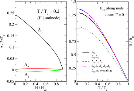
Figure 4: (Color online) Multiple Landau level contributions to the order parameter. Left panel: LL components as a function of the field in the antinodal direction for $T/T_{c}=0.2$ (left). Right panel: upper critical field along a node for different number of Landau channels in $\Delta$ (clean limit); $H_{c2}$ has converged for $N\geq 3$. We also show for comparison the $H_{c2}$ as calculated with one channel $\Delta_{0}$ without coordinate rescaling (17).

The main advantage of allowing for the $c$-axis dispersion is the ability to solve the quasiclassical equations in the BPT approximation self-consistently, with respect to both the order parameter as a function of $T,H$, and the impurity self-energy. We take moderate values of the anisotropy, $s=0.25$ and $s=0.5$, for which the vortex structure is still three-dimensional. The latter value yields $H_{c2}$ anisotropy close to that of CeCoI₅. The calculations below are done with three Landau level channels for the order parameter, ${\Delta_{0},\Delta_{2},\Delta_{4}}$. With the rescaling of Appendix A this is sufficient for convergence of the upper critical field. The values of the higher components $\Delta_{2},\Delta_{4}$ are less than $5\%$ of $\Delta_{0}$, see Fig. 4, and addition of further components does not change the results.

For this Fermi surface we solve the linearized self-consistency equation and compute $H_{c2}$ in the basal plane. The anisotropy between nodal and antinodal upper critical fields appears naturally as a result of the $d$-wave symmetry, $H_{c2}^{node}\neq H_{c2}^{antinode}$. The value of $H_{c2}$ is essentially determined by balancing the kinetic energy of the supercurrents vs. the condensation energy, and the former is different for different orientations of the field.

Let us now look at the difference between the self-consistent and non-self-consistent order parameter calculations. For this we again present a phase diagram, Fig. 5, analogous to Fig.2 for the cylindrical FS. Left panel shows the results for the Fermi surface with $r=s=0.5$, and the impurity strength $\Gamma/2\pi T_{c}=0.007$ ($T_{c}/T_{c0}\sim 0.95$, $\ell_{tr}/\xi_{0}\simeq 70$). The values of the critical fields at $T=0$ are $H_{c2}^{antinode}\approx 1.45B_{0}$, $H_{c2}^{node}\approx 1.27B_{0}$ and $H_{c2}^{c}\approx 0.57B_{0}$. This gives the in-plane anisotropy $(H_{c2}^{antinode}-H_{c2}^{node})/H_{c2}^{antinode}\sim 15\%$, and the ratio between the $c$-axis and antinodal directions, $H_{c2}^{c}/H_{c2}^{antinode}=0.4$.

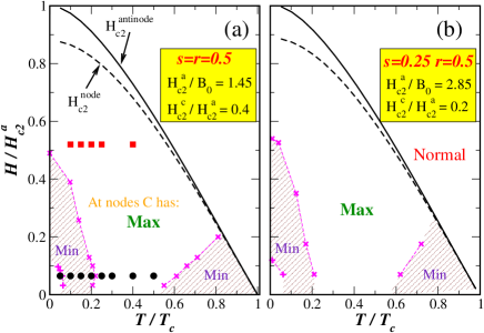
Figure 5: (Color online) The phase diagram of the heat capacity anisotropy $C(\phi_{0})$ for the corrugated FS with $s=r=0.5$ (left) and $s=r/2=0.25$ (right).

To demonstrate the influence of the FS $c$-axis curvature on this phase diagram, we present in Fig. 5(b) a similar diagram a Fermi surface with parameters, $r=0.5$ and $s=0.25$. These parameters correspond to the reduction by factor of 2 of the velocity along the $c$-axis and the critical fields $H_{c2}^{antinode}\approx 2.85B_{0}$, $H_{c2}^{node}\approx 2.55B_{0}$ and $H_{c2}^{c}\approx 0.57B_{0}$. The $H_{c2}$ anisotropies are: 10% in the basal plane between nodal and antinodal directions, and $H_{c2}^{c}/H_{c2}^{antinode}=0.2$. Fig. 5 shows that a factor of two difference in the $c$-axis velocity affects only the absolute values of $H_{c2}^{(anti)node}$, but otherwise the two diagrams for the anisotropy in the $ab$-plane look almost identical.

The shaded “semiclassical” region at low temperatures and fields in Fig. 5, where minima of $C$ are for ${\bf H}||\,node$, expanded compared with that for cylindrical FS (Fig. 2). We note that if we truncate the order parameter expansion at the lowest Landau level, without full convergence of $H_{c2}$, the “nodal minimum” region occupies similar range for both corrugated and purely cylindrical FS. Therefore this expanded range is the result of the self-consistency and inclusion of higher harmonics. On the other hand, the shaded ‘minimum-at-a-node’ region near $H_{c2}$ shrunk to low $H$ and high $T$, where the anisotropy is almost washed out, and is experimentally undetectable.

Specific heat as a function of the field direction is shown in Fig. 6. The curves are computed at the $(T,H)$ points indicated in the phase diagram of Fig. 5 by circles and squares. The left (right) panel refers to lower (higher) field. At higher fields the gap nodes always correspond to maxima of $C$. At low fields, however, nodes correspond to either minima or maxima of $C$ depending on the temperature, Fig. 6(left). The lowest dashed curve in the left panel of Fig. 6 appears to contradict the semiclassical results; we show below that it corresponds to the breakdown of the BPT approximation. We conclude that the optimal range of field and temperature for experimental detection of the nodes based on the heat capacity anisotropy is at intermediate values of $H/H_{c2}$ and $T/T_{c}$, where the anisotropy of $C$ is large and the ambiguity in interpretation is small.

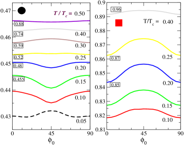
Figure 6: (Color online) Heat capacity profiles for $T$-scans at H= and H=. The gap node is at $\phi_{0}=45^{\circ}$. Left: the evolution of anisotropy with temperature along a line of circles (low field) in Fig.5(a). Right: same for the high field (squares in Fig.5(a)). The curves that were shifted down to appear on the same scale are shown with their original values at $\phi_{0}=0$ in boxes.

The discrepancy between $t=0.5$ profile on the left that shows a weak minimum at the nodes and the position of the point in the ‘maximum’ region of the phase diagram in Fig. 5 is due to the fact that we computed and differentiated entropy to determine the phase diagram, but employed the approximate formula Eq. (38) to calculate the heat capacity anisotropy profile (neglecting the derivative of the DOS with temperature). Comparison of the exact and approximate formulas for the heat capacity is shown in Fig. 7. The lower inversion between the minimum and the maximum of $C$ for the field along the nodes is only slightly shifted to higher $T$ due to use of the approximate formula (inset). The point of the high-$T$ inversion is more sensitive to it, but, as discussed above, is not in the regime of experimental interest.

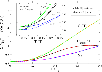
Figure 7: (Color online) The heat capacity at $H/H_{c2}=0.27$. Comparison of the approximate formula Eq. (38) with the rigorous calculation of $C/T=\partial S/\partial T$ from numerical differentiation of the entropy. The crossing of $C$’s for nodal and antinodal ${\bf H}$ directions at low temperature $T/T_{c}\approx 0.15$, indicated by arrows in the inset, is not significantly affected by the approximation.

At the lowest fields and temperatures in Fig. 5 (below 0.1$H_{c2}$ and 0.07$T_{c}$) there appears a very small anomalous region where the heat capacity anisotropy is inverted compared to the semiclassical result. Our analysis shows that this is an artefact caused by the breakdown of the BPT approximation. Manifestations of this failure are enhanced (compared to cylindrical FS) by the fully self-consistent calculation of the multiple Landau channel order parameter.

A necessary condition for the validity of the BPT approximation is that the electron mean free path is much greater than the intervortex distance, $\ell(H)=v_{f}\tau(H)\gg\Lambda(H)$. Only in this case we are allowed to carry out the vortex lattice spatial averaging before averaging over the impurity configurations to compute the self-energy. Consequently, for finite impurity concentration the approximation is bound to fail at low fields. In figure 8 we present the DOS at low field and temperature for different number of $\Delta$-channels and the purity of the material. Notice that for the dirtier material with more than one channel of the order parameter the DOS oscillates at low energies when the field ${\bf H}$ is $||\,antinode$, panel (b). These oscillations lead to the additional unphysical inversion of the heat capacity anisotropy at very low $T,H$, that is seen in the bottom left corner of the phase diagram in Fig. 5, and is shown by the dashed line in the left panel of Fig. 6. The same oscillations are also present in the self-consistently calculated impurity self-energies, which we do not show here. We find that they decrease in a cleaner material, Fig. 8(c).

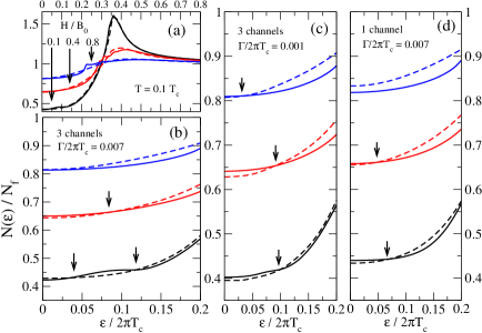
Figure 8: (Color online) The DOS for quasi-cylindrical FS for fields $H/B_{0}=0.1,0.4,0.8$ ($H_{c2}=1.45B_{0}(1.27B_{0})$ for ${\bf H}||\,$antinode (node)). (a) Overall shape of the DOS for three fields, and (b) enlarged low-energy region. The low field DOS for nodal (dashed) and antinodal (solid) directions of ${\bf H}$ cross several times. We ascribe it to high derivatives of $W$-function. The oscillating behavior decreases as system becomes cleaner (c), and disappears for single channel (d).

The interval of the fields where the oscillations are observed coincides with the region where the BPT approximation is no longer trustable. We consider the BPT breakdown at low temperature, where the density of states is, Eq. (40), $N(0,H)/N_{0}=-\mathfrak{Im}\,\langle g/\pi\rangle\sim\sqrt{H/H_{c2}}$. The impurity self-consistency in the unitary limit gives $\tau(H)={1\over 2\gamma}\;N(0,H)/N_{0}\sim{1\over 2\gamma}\,\sqrt{H\over H_{c2}}$. Here $\gamma=\Gamma\sin^{2}\delta_{0}$ is the normal state scattering rate. Recalling that $\Lambda(H)/\xi_{0}\sim\sqrt{H_{c2}/H}$ and requiring $v_{f}\tau(H)\gg\Lambda(H)$, we obtain a condition for the applicability of BPT: $H/H_{c2}\gg\gamma/2\pi T_{c}$. Thus, for our impurity bandwidth $\gamma/2\pi T_{c}\sim 0.01$ the BPT approximation is only applicable for fields $H/H_{c2}\gg 0.01$ and the oscillations seen in the DOS likely are a signature of this breakdown. We checked that increasing disorder expands the anomalous region and is consistent with this interpretation. For the single-component (lowest Landau level) $\Delta$, the numerically computed DOS does not show significant anomalous behavior, Fig. 8(d), at the same impurity level as in Fig. 8(b). We argue that although the breakdown of the approximation is still there, its manifestation is less pronounced compared with the multiple-channel order parameter. Use of higher Landau channels for the expansion of $\Delta$ leads to the appearance of the higher derivatives of the $W(z)$-function, $W^{(n)}(z)$, in the Green’s function, see (Eq.33). These grow very fast with $n$ at $z=0$ (approximately as $n!!$) and are strongly oscillating as the argument is increased from zero. This is likely the underlying reason for the oscillations in the DOS, and therefore the ultra-low $T$-$H$ inversion is an artefact of using the approximation beyond its region of validity. In contrast, other inversion lines in the phase diagram correspond to physical inversion of the measured properties.

V Discussion and conclusions

In this work we laid the foundations for an approach that provides a highly flexible basis to the calculation, on equal footing, of the transport and thermodynamic properties of unconventional superconductors under magnetic field. The theoretical method is based on the quasiclassical theory of superconductivity and the Brandt-Pesch-Tewordt approximation for treatment of the vortex state in superconductors. This approximation allows for accurate and straightforward (analytic closed form expressions for the Green’s functions) way to describe effects of the magnetic field in almost the entire $T$-$H$ phase diagram for clean superconductors, with the exception of ultralow fields and temperatures. Combined with the non-equilibrium Keldysh formulation of the quasiclassical theory it paves a path for a very effective computational scheme that self-consistently takes into account multiple Landau levels of the expansion of the order parameter and impurities, and allows calculations for arbitrary temperature and magnitude of the field. The companion paper II extends the method to the calculation of transport properties and focuses on the electronic thermal conductivity.

Here we computed the density of states and the specific heat in the $T$-$H$ plane for a $d$-wave superconductor with a quasi-two dimensional Fermi surface (cylinder modulated along the symmetry axis), and the magnetic field rotated in the basal plane. This choice of the Fermi surface and the field orientation was motivated by experiments on the heavy fermion CeCoIn₅ Aoki et al. (2004). We provided the first complete description of the evolution of the anisotropy of the heat capacity due to nodes of the superconducting gap across the $T$-$H$ phase diagram, see Fig. 9.

Our main conclusion is that the anisotropic scattering of quasiparticles due to vortices plays a crucial role in the variation of the density of states and the specific heat as a function of the field direction. This effect is absent in the semiclassical (Doppler shift) approach, and becomes important already at moderately low fields, and at finite temperatures. As our phase diagram of Fig. 9 shows, as a result of this scattering, the anisotropy in the specific heat changes sign as a function of $T$ and $H$. At low fields and temperatures the minima in the heat capacity occur when the field is oriented along the nodal directions, in agreement with the semiclassical (Doppler shift) calculation. At higher $T$ and $H$ (already at $T/T_{c}\gtrsim 0.2$ at low fields) the situation is reversed, and the maxima rather than minima of the specific heat are found when the field is along a nodal direction. Moreover, we showed that the inversion is related to the behavior of the density of states at finite energy, and not simply the residual DOS at the Fermi surface.

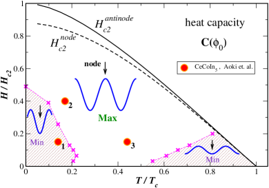
Figure 9: (Color online) The anisotropy of the heat capacity in rotated magnetic field. The $T$-$H$ phase diagram for a $d$-wave superconductor with a corrugated cylinder Fermi surface with purely orbital depairing. In the large part of the phase diagram the maxima of $C(\phi_{0})$ function correspond the nodal directions (indicated by arrows) on the Fermi surface. This result is opposite to that in the Doppler region, which is confined to $H/H_{c2}\lesssim 0.5$ and $T/T_{c}\lesssim 0.2$.

While we expect that the loci of the inversion lines in the $T$-$H$ plane weakly depend on the shape of the Fermi surface Udagawa et al. (2005), it is the existence of this inversion and its connection to the scattering and the finite energy DOS that emerged from our theoretical description and was not captured by previous approaches to the problem. Our calculations serve as a basis for the analysis of the experimental data, and we note that the interpretation of experiments based on the low-field expectations of minima for the field along the nodes can lead to diametrically opposite conclusions regarding the gap symmetry, depending on the values of the field and temperature where the anisotropy is been measured. The results suggest that the amplitude of the anisotropy is the greatest at intermediate temperatures and fields, and that it is desirable not only to measure the $C$ anisotropy at a few temperatures and fields, but also determine its evolution over the phase diagram.

As an example, we consider the data for CeCoIn₅ from Ref. Aoki et al., 2004, and plot in Fig. 9 the points where the published data were taken. The measured $C(\phi_{0})$ shows minima for the field along the [100] and [010] directions ($\phi_{0}=\pi n/2$ with $n=0,1,2,3$), at all three locations, with vanishingly small anisotropy at point 3. Points 2 and 3 are clearly in the region where maxima of $C(\phi_{0})$ determine the nodes, and thus firmly point towards $d_{x^{2}-y^{2}}$ symmetry. Point 3 is also close to the inversion line, which explains small amplitude of the oscillations. Point 1, in contrast, is in the “semiclassical” region, and therefore the minima of $C(\phi_{0})$ for the field along the crystal axes may be more suggestive of a $d_{xy}$ symmetry. We note, however, that the exact location of the inversion line is sensitive to the exact shape of the Fermi surface, and changes between the calculations restricted to the lowest Landau level for cylindrical Fermi surface, Fig. 2 and the multicomponent quasi-2D case, Fig. 5. We argue therefore that points 2 and 3 are more reliable indicators of the gap symmetry, and the results are more suggestive of the $d_{x^{2}-y^{2}}$ gap. While such a conclusion purely from the specific heat data is not foolproof, we show in II that the $d_{x^{2}-y^{2}}$ symmetry is also supported by the analysis of the heat transport anisotropy of Ref. Izawa et al., 2001.

The microscopic approach, by its very nature, couples the gap symmetry with the shape of the Fermi surface. For that reason direct comparison of our results with other experimental data, for example in the borocarbides YNi₂B₂CPark et al. (2003) and LuNi₂B₂CPark et al. (2004), is not possible. These systems are essentially three dimensional, and the Fermi surface has no quasi-cylindrical sheets. Moreover, it is very likely that there is substantial gap modulation along the $z$-axis, and comparison should be made with both point and line node models Park et al. (2003); Izawa et al. (2002b). While the argument for the change in the anisotropy due to scattering on the vortices is quite general, the position of the anisotropy inversion lines in the phase diagram (if any) is undoubtedly different from that found for the quasi-2D system, and such differences are known to occur in the zero-energy DOS  Udagawa et al. (2005). Therefore we will consider the nodal structures of these systems separately in near future.

To reiterate, the approach described in this work presents a powerful tool to study the gap symmetry in the unconventional superconductors taking into account their realistic Fermi surfaces. Our results serve as a basis for interpretation of experimental data, pointing towards a resolution of the discrepancy between the results of the specific heat and thermal conductivity measurements in CeCoIn₅, which is also addressed in II. The method developed here can be easily generalized to include other Fermi surfaces, paramagnetic effects, and other aspects of real materials, the discussion of which we defer to future publications.

VI Acknowledgements

This work was partly done at KITP with support from NSF Grant PHY99-07949; and was also supported by the Board of Regents of Louisiana. We thank D. A. Browne, C. Capan, P. J. Hirschfeld, Y. Matsuda, and T. Sakakibara for discussions, and one of us (I. V) is very indebted to A. Houghton for encouragement at the early stages of this work.

Appendix A Choice of operators for anisotropic Fermi surface

The raising and lowering operators for the eigenfunction expansion of the order parameter, $a^{\dagger},a$ and the corresponding ladder states can be introduced in several different ways. We want to define them in the manner that facilitates the efficient computations. This issue becomes important for anisotropic Fermi surfaces and arbitrary direction of the field. Anisotropy of the FS is directly translated into the shape of a single vortex and we can choose the orthogonal states such that they approximate this shape well already at the lowest order truncation of the expansion of $\Delta(\bm{R})$.

We consider an axisymmetric FS in cylindrical coordinates $(r,\phi,z_{0})$. The energy has the form $2m\varepsilon=p_{r}^{2}+f(p_{z_{0}})$, with an arbitrary function $f(p_{z_{0}})$ of the $p_{z_{0}}$ momentum. The vortex state near the critical temperature $T_{c}$ is determined from the linearized GL equations,

$$-K_{ij}\tilde{\mbox{\boldmath$\nabla$}}_{i}\tilde{\mbox{\boldmath$\nabla$}}_{j}\Delta({\bf R})+\left({T\over T_{c}}-1\right)\Delta({\bf R})=0$$ (49)

$$K_{ij}=T_{c}\sum_{\varepsilon_{m}}{\pi\over 4|\varepsilon_{m}|^{3}}\langle{\cal Y}^{2}(\hat{{\bf p}})v_{f,i}(\hat{{\bf p}})v_{f,j}(\hat{{\bf p}})\rangle_{\mbox{\tiny FS}}$$ (50)

$$\tilde{\mbox{\boldmath$\nabla$}}=\mbox{\boldmath$\nabla$}-i{2e\over c}{\bf A}({\bf R})$$ (51)

In these equations the coordinates $(x,y,z)$ are chosen so that the field is along the $z$-axis, ${\bf B}=B\hat{{\bf z}}$, and we take ${\bf A}=(0,Bx,0)$. The form of the $K_{ij}$ tensor depends on the shape of the Fermi surface, the pairing state and orientation of the magnetic field. If the rotational symmetry axis is $z_{0}$, the velocity of quasiparticles is ${\bf v}_{f}(\phi,p_{z_{0}})=(v_{r}(p_{z_{0}})\cos\phi,v_{r}(p_{z_{0}})\sin\phi,v_{z_{0}}(p_{z_{0}}))$. If ${\bf B}$ is along one of the FS symmetry axes, $x_{0}$, $y_{0}$ or $z_{0}$, $K_{ij}$ is diagonal for $d$-wave pairing with ${\cal Y}=\sqrt{2}\cos 2(\phi-\phi_{0})$. We have, $K_{x_{0}x_{0}}=K_{y_{0}y_{0}}=K_{0}v_{0\perp}^{2}$, $K_{z_{0}z_{0}}=K_{0}v_{0||}^{2}$, where $K_{0}=7\zeta(3)/8(2\pi T_{c})^{2}$, and

$$v_{0\perp}^{2} = 2\,\langle{\cal Y}^{2}(\hat{{\bf p}})v^{2}_{x_{0}(y_{0})}(p_{z_{0}})\rangle_{\mbox{\tiny FS}}\,,$$ (52)

$$v_{0\parallel}^{2} = 2\,\langle{\cal Y}^{2}(\hat{{\bf p}})v^{2}_{z_{0}}(p_{z_{0}})\rangle_{\mbox{\tiny FS}}\,.$$ (53)

We apply the magnetic field at a tilt angle $\theta_{H}$ from $z_{0}$ direction towards $x_{0}$ axis. A coordinate system associated with ${\bf B}$ is chosen as follows, $\hat{z}$ is along ${\bf B}$, $\hat{y}=\hat{y}_{0}$ and $\hat{x}$ lies in $(x_{0},z_{0})$-plane and perpendicular to $\hat{z}$. Projections of the Fermi velocity at different points of the FS on these new coordinate axes, $v_{f,x}(p_{z_{0}},\phi)=v_{f,x_{0}}(p_{z_{0}},\phi)\cos\theta_{H}-v_{f,z_{0}}(p_{z_{0}},\phi)\sin\theta_{H}$, $v_{f,y}(p_{z_{0}},\phi)=v_{f,y_{0}}(p_{z_{0}},\phi)$, $v_{f,z}(p_{z_{0}},\phi)=v_{f,z_{0}}(p_{z_{0}},\phi)\cos\theta_{H}+v_{f,x_{0}}(p_{z_{0}},\phi)\sin\theta_{H}$. In $(x,y,z)$-coordinates the tensor $K_{ij}$ is not diagonal anymore, $K_{yy}=K_{y_{0}y_{0}}$, $K_{xx}=K_{x_{0}x_{0}}\cos^{2}\theta_{H}+K_{z_{0}z_{0}}\sin^{2}\theta_{H}$, $K_{zz}=K_{x_{0}x_{0}}\sin^{2}\theta_{H}+K_{z_{0}z_{0}}\cos^{2}\theta_{H}$, $K_{xz}=(K_{x_{0}x_{0}}-K_{z_{0}z_{0}})\sin\theta_{H}\cos\theta_{H}$, and for the choice of the operator, $\mbox{\boldmath$\nabla$}-i2e/c\,{\bf A}=(\mbox{\boldmath$\nabla$}_{x},\mbox{\boldmath$\nabla$}_{y}-i2e/c\,Bx,\mbox{\boldmath$\nabla$}_{z})$, the GL equation is

$$-K_{xx}\mbox{\boldmath$\nabla$}^{2}_{x}\;\Delta-K_{yy}\left(\mbox{\boldmath$\nabla$}_{y}-i{2eB\over c}x\right)^{2}\;\Delta$$

$$-2K_{xz}\mbox{\boldmath$\nabla$}_{x}\mbox{\boldmath$\nabla$}_{z}\;\Delta+\left({T\over T_{c}}-1\right)\;\Delta=0\,.$$ (54)

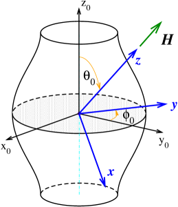
Figure 10: (Color online) Quasi-cylindrical Fermi surface considered in this paper. Direction of ${\bf H}$ defines $(xyz)$ coordinates with $\hat{{\bf z}}||{\bf H}$. To go from $(x_{0}y_{0}z_{0})$ coordiantes, associated with the Fermi surface, to $(xyz)$ coordinates, associated with the field, we perform first rotation by $\phi_{0}$ around $\hat{{\bf z}}_{0}$, and then rotation by $\theta_{0}$ around $\hat{{\bf y}}$.

It is easy to check by setting $\Delta=\Delta(x,y)\exp(ik_{z}z)$ that the highest critical field still corresponds to $k_{z}=0$, and we put $\mbox{\boldmath$\nabla$}_{z}\Delta=0$ below. We rescale the coordinates $x^{\prime}=x/\sqrt{S_{f}}$ and $y^{\prime}=y\sqrt{S_{f}}$, and choose the scaling factor $S_{f}$ such that $K_{xx}/S_{f}=K_{yy}S_{f}$. Thus,

$$S_{f}^{2}={K_{xx}\over K_{yy}}=\cos^{2}\theta_{H}+\frac{v_{0\|}^{2}}{v_{0\perp}^{2}}\sin^{2}\theta_{H}\,.$$ (55)

After introducing creation and annihilation operators ($\Lambda^{2}=c/2|e|B$ and $e<0$),

$$a={\Lambda\over\sqrt{2}}\left(-\mbox{\boldmath$\nabla$}_{x^{\prime}}+i(\mbox{\boldmath$\nabla$}_{y^{\prime}}+i{x^{\prime}\over\Lambda^{2}})\right)\,,$$ (56)

$$a^{\dagger}={\Lambda\over\sqrt{2}}\left(\mbox{\boldmath$\nabla$}_{x^{\prime}}+i(\mbox{\boldmath$\nabla$}_{y^{\prime}}+i{x^{\prime}\over\Lambda^{2}})\right)\,,$$ (57)

equation (54) becomes

$$\left(a^{\dagger}a+{1\over 2}\right)\Delta(x,y)={\Lambda^{2}\over 2}{S_{f}\over K_{xx}}\left(1-{T\over T_{c}}\right)\;\Delta(x,y)\,.$$ (58)

Then for any axisymmetric FS we obtain the well-known result of the anisotropic mass model for the upper critical field, determined by the ratio of the Fermi velocities for the two directions,

$$B_{c2}(\theta_{H},T)={const\cdot(1-T/T_{c})\over\sqrt{\cos^{2}\theta_{H}+{v_{0||}^{2}\over v_{0\perp}^{2}}\sin^{2}\theta_{H}}}\,.$$ (59)

We also find a set of eigenfunctions,

$$\Delta^{(n)}(x,y)=\sum_{k_{y}}C_{k_{y}}^{(n)}{e^{ik_{y}\sqrt{S_{f}}y}\over\sqrt[4]{S_{f}\Lambda^{2}}}\Phi_{n}\left({x-\Lambda^{2}\sqrt{S_{f}}k_{y}\over\Lambda\sqrt{S_{f}}}\right)\,.$$ (60)

In terms of the operators ${a,a^{\dagger}}$ the gradient term in the Eilenberger equation has the form

$${\bf v}_{f}(\hat{{\bf p}})\,(\mbox{\boldmath$\nabla_{\mbox{\tiny${\bf R}$}}$}-i{2e\over c}{\bf A}({\bf R}))=$$ (61)

$${|\tilde{v}_{f}^{\perp}|\over\sqrt{2}\Lambda}[-\tilde{v}_{+}(\hat{{\bf p}})\,a+\tilde{v}_{-}(\hat{{\bf p}})\,a^{\dagger}]\,.$$

Here we rescaled the Fermi velocity in the $xy$-plane

$$\tilde{v}_{f}(\hat{{\bf p}})_{x} = v_{f}(\hat{{\bf p}})_{x}/\sqrt{S_{f}}\,,$$ (62)

$$\tilde{v}_{f}(\hat{{\bf p}})_{y} = v_{f}(\hat{{\bf p}})_{y}\sqrt{S_{f}}\,,$$ (63)

with

$$|\tilde{v}_{f}^{\perp}(\hat{{\bf p}})|=\sqrt{\tilde{v}_{f}(\hat{{\bf p}})_{x}^{2}+\tilde{v}_{f}(\hat{{\bf p}})_{y}^{2}}\,,$$ (64)

and

$$\tilde{v}_{\pm}(\hat{{\bf p}})=\frac{\tilde{v}_{f}(\hat{{\bf p}})_{x}\pm i\tilde{v}_{f}(\hat{{\bf p}})_{y}}{|\tilde{v}_{f}^{\perp}|}\,.$$ (65)

Appendix B Closed form solution for the Green’s function

To solve the semiclassical equations we use Eq. (61) to cast the operator $\hat{O}_{f}$ from Eq. (15) in an integral form,

$$\hat{O}_{f} = [-2i\tilde{\varepsilon}+{|\tilde{v}^{\perp}_{f}|\over\sqrt{2}\Lambda}(\tilde{v}_{-}a^{\dagger}-\tilde{v}_{+}a)]^{-1}$$ (66)

$$= \int\limits_{0}^{\infty}dt_{1}\;e^{-[-2i\tilde{\varepsilon}+{|\tilde{v}^{\perp}_{f}|\over\sqrt{2}\Lambda}(\tilde{v}_{-}a^{\dagger}-\tilde{v}_{+}a)]t_{1}}$$

$$= \int\limits_{0}^{\infty}dt_{1}\;e^{2i\tilde{\varepsilon}t_{1}-{w^{2}}t_{1}^{2}/2}e^{-wt_{1}\,\tilde{v}_{-}a^{\dagger}}e^{wt_{1}\,\tilde{v}_{+}a}\,,$$

where we introduced the magnetic field energy

$$w={|\tilde{v}^{\perp}_{f}|\over\sqrt{2}\Lambda}\,$$ (67)

and used the operator identity $\exp(A+B)=\exp(A)\exp(B)\exp(-C/2)$, if $[A,B]=C$ is a $c$-number. In all integrals we also keep in mind that $\mathfrak{Im}\,\tilde{\varepsilon}>0$ for retarded functions, so that the convergence is ensured.

In this formulation it is convenient to work with bra- and ket-functions for different vortex states, which correspond in ${\bf R}$-representation to states (60). We present decomposition of $\tilde{\Delta}$ as

$$\widetilde{\Delta}=\sum_{n}\widetilde{\Delta}_{n}\mbox{$\displaystyle|\,n\,\rangle$}\,,\qquad\widetilde{\underline{\Delta}}=\sum_{n}\widetilde{\underline{\Delta}}_{n}\mbox{$\displaystyle\langle\,n\,|$}\,,$$ (68)

with operator $\hat{O}_{f}$ acting to the right,

$$f = (2ig)\,\hat{O}_{f}\widetilde{\Delta}=$$

$$= (2ig)\int\limits_{0}^{\infty}dt_{1}\,e^{2i\tilde{\varepsilon}t_{1}-{w^{2}}t_{1}^{2}/2}e^{-wt_{1}\,\tilde{v}_{-}a^{\dagger}}e^{wt_{1}\,\tilde{v}_{+}a}\widetilde{\Delta}\,,$$

and operator $\hat{O}_{\underline{f}}^{\dagger}$ acting to the left,

$$\underline{f}=(2ig)\,\widetilde{\underline{\Delta}}\,\hat{O}_{\underline{f}}^{\dagger}\,.$$ (70)

We rewrite the operator $\hat{O}_{\underline{f}}$ as

$$\hat{O}_{\underline{f}} = [2i\tilde{\varepsilon}^{*}-w(\tilde{v}_{-}a^{\dagger}-\tilde{v}_{+}a)]^{-1}=\hat{O}^{\dagger}_{f}=$$

$$= \int\limits_{0}^{\infty}dt_{2}\;e^{-2i\tilde{\varepsilon}^{*}t_{2}-{w^{2}}t_{2}^{2}/2}e^{wt_{2}\,\tilde{v}_{-}a^{\dagger}}e^{-wt_{2}\,\tilde{v}_{+}a}\,.$$

so that the spatial average of the off-diagonal functions is

$$\overline{\underline{f}\,f} = (2ig)^{2}\int\limits_{0}^{\infty}dt_{1}\,\int\limits_{0}^{\infty}dt_{2}\;e^{2i\tilde{\varepsilon}(t_{1}+t_{2})-{w^{2}}(t_{1}+t_{2})^{2}/2}\times$$ (72)

$$\times \widetilde{\underline{\Delta}}\left(e^{-w(t_{1}+t_{2})\,\tilde{v}_{-}a^{\dagger}}e^{w(t_{1}+t_{2})\,\tilde{v}_{+}a}\right)\widetilde{\Delta}\,,$$

where we make sure that bra-vectors stay on the left of ket-vectors. Here we again used operator-in-exponent rule to commute exponents. After an appropriate variable susbstitution,

$$\overline{\underline{f}\,f}=(2ig)^{2}\int\limits_{0}^{\infty}dt\;t\,e^{2i\tilde{\varepsilon}t-{w^{2}}t^{2}/2}\widetilde{\underline{\Delta}}\left(e^{-wt\,\tilde{v}_{-}a^{\dagger}}e^{wt\,\tilde{v}_{+}a}\right)\widetilde{\Delta}\,.$$ (73)

This form is very convenient if we intend to keep several Landau channels in the expansion of $\Delta$. If the highest Landau level used is $N$, the series expansion for $e^{wt\,\tilde{v}_{+}a}$ contains only $N+1$ terms; and to calculate the spatial average $\overline{\underline{f}\,f}$ we need to compute only a finite number, ($2N+1$), of $W^{(n)}$-functions, since

$$\int\limits_{0}^{\infty}dt\;t\,(wt)^{n}\,e^{2i\tilde{\varepsilon}t-{w^{2}}t^{2}/2}=$$ (74)

$$={1\over 2w^{2}}(-i\sqrt{\pi})\left(-{i\over\sqrt{2}}\right)^{n}W^{(n+1)}\left({\sqrt{2}\tilde{\varepsilon}\over w}\right)\,.$$

Solution for $f$ is written as,

$$f({\bf R},\hat{{\bf p}};\varepsilon)=\sum_{m}f_{m}(\hat{{\bf p}},\varepsilon)\mbox{$\displaystyle\langle\,{\bf R}\,|\,m\,\rangle$}\,,$$ (75)

with the amplitudes

$$f_{m}(\hat{{\bf p}},\varepsilon)=ig\,\sum_{n}(-\tilde{v}_{-})^{m-n}(\hat{{\bf p}})\,{\cal D}_{m,n}(\varepsilon,|\hat{{\bf p}}|)\widetilde{\Delta}_{n}(\hat{{\bf p}};\varepsilon)\,.$$ (76)

Here

$${\cal D}_{m,n}(\varepsilon,|\hat{{\bf p}}|)={2\sqrt{\pi}\Lambda\over|\tilde{v}^{\perp}_{f}|}\sum_{n_{2}}^{m}(-1)^{n_{1}}D_{n}^{n_{1},n_{2}}\left({2\tilde{\varepsilon}\Lambda\over|\tilde{v}^{\perp}_{f}|}\right)\,,$$ (77)

$$D^{n_{1},n_{2}}_{n}(z)=\left({-i\over\sqrt{2}}\right)^{n_{1}+n_{2}}{\sqrt{n!}\sqrt{(n-n_{1}+n_{2})!}\over(n-n_{1})!n_{1}!n_{2}!}W^{(n_{1}+n_{2})}(z).$$ (78)

The sum starts from $n_{2}=max(0,m-n)$ and, in each term, $n_{1}=n-m+n_{2}$. This sum can be cast in a more symmetric form with respect to the indices $m,n$, which we present in the main text in Eq.(31).

We limit ourselves to superconductors with inversion symmetry. Then the singlet and triplet order parameters transform under inversion as follows,

$${\cal P}\Delta({\bf R},\hat{{\bf p}})=\Delta(-{\bf R},-\hat{{\bf p}})=\Delta({\bf R},-\hat{{\bf p}})=\Delta({\bf R},\hat{{\bf p}})\,,$$

$${\cal P}\mbox{\boldmath$\Delta$}({\bf R},\hat{{\bf p}})=\mbox{\boldmath$\Delta$}(-{\bf R},-\hat{{\bf p}})=\mbox{\boldmath$\Delta$}({\bf R},-\hat{{\bf p}})=-\mbox{\boldmath$\Delta$}({\bf R},\hat{{\bf p}})\,,$$

where we assumed that the order parameter is an even function of the spatial coordinates ${\bf R}$. This assumption is justified by the analysis of the behavior of the off-diagonal functions $f_{m}(\hat{{\bf p}})$. The expansion of the anomalous propagators in the Landau level basis contains all components $\langle{\bf R}|m\rangle$, however, even and odd coefficients have different parity under inversion ${\bf p}\rightarrow-{\bf p}$,

$$f^{s}_{m}(-\hat{{\bf p}})=ig\,\sum_{n}\tilde{v}_{-}^{m-n}(\hat{{\bf p}})\,{\cal D}_{m,n}(|\hat{{\bf p}}|)\widetilde{\Delta}_{n}(\hat{{\bf p}})\,,$$

$$f^{t}_{m}(-\hat{{\bf p}})=-ig\,\sum_{n}\tilde{v}_{-}^{m-n}(\hat{{\bf p}})\,{\cal D}_{m,n}(|\hat{{\bf p}}|)\mbox{\boldmath$\Delta$}_{n}(\hat{{\bf p}})\,.$$

As a result, it is easy to show that for both singlet and triplet order parameters, the even and odd coefficients $\Delta_{n}$ are decoupled since no mixed term survives averaging over the Fermi surface,

$$\int\frac{d\Omega_{\hat{p}}}{4\pi}{\cal Y}_{s,t}(\hat{{\bf p}})f^{s,t}(\hat{{\bf p}}).$$ (79)

Note also that, in zero field for superconductors with basis functions $\langle{\cal Y}(\hat{{\bf p}})\rangle_{\mbox{\tiny FS}}=0$, the off-diagonal impurity self-energy vanishes since $\langle f(\hat{{\bf p}})\rangle_{\mbox{\tiny FS}}=0$. Under magnetic field, however, the direction $\hat{{\bf p}}$ is inequivalent to the perpendicular to it direction, $\hat{{\bf p}}_{\perp}$, and $f(\hat{{\bf p}})$ is not simply proportional to ${\cal Y}(\hat{{\bf p}})$. Hence for the field in the plane and $d$-wave gap $\langle f(\hat{{\bf p}})\rangle_{\mbox{\tiny FS}}\neq 0$, and there is a contribution to the off-diagonal self-energies from impurities. This integral still vanishes for $p$-wave order parameters, since in magnetic field the directions $\hat{{\bf p}}$ and $-\hat{{\bf p}}$ may remain equivalent and so the symmetry $f(-\hat{{\bf p}})=-f(\hat{{\bf p}})$ is still valid.

References

- Vorontsov and Vekhter (2007) A. Vorontsov and I. Vekhter, (unpublished).
- Sigrist and Ueda (1991) M. Sigrist and K. Ueda, Rev. Mod. Phys. 63, 239 (1991).
- Vekhter et al. (1999) I. Vekhter, P. J. Hirschfeld, E. J. Nicol, and J. P. Carbotte, Phys. Rev. B 59, R9023 (1999).
- Yip and Sauls (1992) S. K. Yip and J. A. Sauls, Phys. Rev. Lett. 69, 2264 (1992).
- Volovik (1993) G. E. Volovik, JETP Letters 58, 469 (1993).
- Xu et al. (1995a) D. Xu, S. K. Yip, and J. A. Sauls, Phys. Rev. B 51, 16233 (1995a).
- Yu et al. (1995) F. Yu, M. B. Salamon, A. J. Leggett, W. C. Lee, and D. M. Ginsberg, Phys. Rev. Lett. 74, 5136 (1995), [Erratum ibid. 75, 3028].
- Aubin et al. (1997) H. Aubin, K. Behnia, M. Ribault, R. Gagnon, and L. Taillefer, Phys. Rev. Lett. 78, 2624 (1997).
- Watanabe et al. (2004) T. Watanabe, K. Izawa, Y. Kasahara, Y. Haga, Y. Onuki, P. Thalmeier, K. Maki, and Y. Matsuda, Phys. Rev. B 70, 184502 (2004).
- Izawa et al. (2001) K. Izawa, H. Yamaguchi, Y. Matsuda, H. Shishido, R. Settai, and Y. Onuki, Phys. Rev. Lett. 87, 057002 (2001).
- Izawa et al. (2003) K. Izawa, Y. Nakajima, J. Goryo, Y. Matsuda, S. Osaki, H. Sugawara, H. Sato, P. Thalmeier, and K. Maki, Phys. Rev. Lett. 90, 117001 (2003).
- Izawa et al. (2002a) K. Izawa, H. Yamaguchi, T. Sasaki, and Y. Matsuda, Phys. Rev. Lett. 88, 027002 (2002a).
- Izawa et al. (2002b) K. Izawa, K. Kamata, Y. Nakajima, Y. Matsuda, T. Watanabe, M. Nohara, H. Takagi, P. Thalmeier, and K. Maki, Phys. Rev. Lett. 89, 137006 (2002b).
- Matsuda et al. (2006) Y. Matsuda, K. Izawa, and I. Vekhter, J.Phys.: Cond.Mat. 18, R705 (2006).
- Park et al. (2003) T. Park, M. B. Salamon, E. M. Choi, H. J. Kim, and S.-I. Lee, Phys. Rev. Lett. 90, 177001 (2003).
- Park et al. (2004) T. Park, E. E. M. Chia, M. B. Salamon, E. D. Bauer, I. Vekhter, J. D. Thompson, E. M. Choi, H. J. Kim, S.-I. Lee, and P. C. Canfield, Phys. Rev. Lett. 92, 237002 (2004).
- Aoki et al. (2004) H. Aoki, T. Sakakibara, H. Shishido, R. Settai, Y. Onuki, P. Miranović, and K. Machida, Journal of Physics: Condensed Matter 16, L13 (2004).
- Kübert and Hirschfeld (1998a) C. Kübert and P. J. Hirschfeld, Solid State Commun. 105, 459 (1998a).
- Kübert and Hirschfeld (1998b) C. Kübert and P. J. Hirschfeld, Phys. Rev. Lett. 80, 4963 (1998b).
- Franz (1999) M. Franz, Phys. Rev. Lett. 82, 1760 (1999).
- Vekhter and Hirschfeld (2000) I. Vekhter and P. J. Hirschfeld, Physica C 341-348, 1947 (2000).
- Thalmeier and Maki (2002) P. Thalmeier and K. Maki, Europhys. Lett. 58, 119 (2002).
- Kim et al. (2003) W. Kim, F. Marsiglio, and J. P. Carbotte, Phys. Rev. B 68, 174513 (2003).
- Udagawa et al. (2004) M. Udagawa, Y. Yanase, and M. Ogata, Phys. Rev. B 70, 184515 (2004).
- Brandt et al. (1967) U. Brandt, W. Pesch, and L. Tewordt, Z. Phys. 201, 209 (1967).
- Vekhter and Houghton (1999) I. Vekhter and A. Houghton, Phys. Rev. Lett. 83, 4626 (1999).
- Dahm et al. (2002) T. Dahm, S. Graser, C. Iniotakis, and N. Schopohl, Phys. Rev. B 66, 144515 (2002).
- Eilenberger (1968) G. Eilenberger, Z. Phys. 214, 195 (1968).
- Larkin and Ovchinnikov (1969) A. I. Larkin and Y. N. Ovchinnikov, Sov. Phys. JETP 28, 1200 (1969).
- Pesch (1975) W. Pesch, Z. Phys. B 21, 263 (1975).
- Houghton and Vekhter (1998) A. Houghton and I. Vekhter, Phys. Rev. B 57, 10831 (1998).
- Vorontsov and Vekhter (2006) A. B. Vorontsov and I. Vekhter, Phys. Rev. Lett. 96, 237001 (2006).
- Serene and Rainer (1983) J. W. Serene and D. Rainer, Phys. Rep. 101, 221 (1983).
- Alexander et al. (1985) J. Alexander, T. Orlando, D. Rainer, and P. Tedrow, Phys. Rev. B 31, 5811 (1985).
- Eschrig et al. (1999) M. Eschrig, J. A. Sauls, and D. Rainer, Phys. Rev. B 60, 10447 (1999).
- Hirschfeld et al. (1988) P. J. Hirschfeld, P. Wölfle, and D. Einzel, Phys. Rev. B 37, 83 (1988).
- Löfwander and Fogelström (2004) T. Löfwander and M. Fogelström, Phys. Rev. B 70, 024515 (2004).
- Vorontsov and Vekhter (2006-7) A. B. Vorontsov and I. Vekhter, xxx 777, Zeeman (2006-7).
- Brandt (1976) E. H. Brandt, J. Low Temp. Phys. 24, 409 (1976).
- Won and Maki (1996) H. Won and K. Maki, Phys. Rev. B 53, 5927 (1996).
- Kusunose (2004) H. Kusunose, Phys. Rev. B 70, 054509 (2004).
- Tewordt and Fay (2005) L. Tewordt and D. Fay, Phys. Rev. B 72, 014502 (2005).
- Tinkham (1985) M. Tinkham, ”Introduction to Superconductivity” (Robert E. Krieger Publishing Co. Malabar, Florida, 1985).
- Li and Rosenstein (1999) D. Li and B. Rosenstein, Phys. Rev. B 60, 9704 (1999).
- Luk’yanchuk and Mineev (1987) I. A. Luk’yanchuk and V. P. Mineev, Zh. Eksp. i Teor. Fiz. 93, 2045 (1987), [Sov. Phys. JETP 66, 1168 (1987)].
- Adachi et al. (2005) H. Adachi, P. Miranović, M. Ichioka, and K. Machida, Phys. Rev. Lett. 94, 067007 (2005).
- Ketterson and Song (1999) J. B. Ketterson and S. N. Song, ”Superconductivity” (Cambridge University Press, 1999).
- Klimesch and Pesch (1978) P. Klimesch and W. Pesch, J. Low Temp. Phys. 32, 869 (1978).
- Xu et al. (1995b) D. Xu, S. K. Yip, and J. A. Sauls, Phys. Rev. B 51, 16233 (1995b).
- Gradshteyn and I.M.Ryzhik (1980) I. Gradshteyn and I.M.Ryzhik, Table of integrals, series, and products (Academic Press, 1980).
- Miranović et al. (2003) P. Miranović, N. Nakai, M. Ichioka, and K. Machida, Phys. Rev. B 68, 052501 (2003).
- Udagawa et al. (2005) M. Udagawa, Y. Yanase, and M. Ogata, Phys. Rev. B 71, 024511 (2005).