Energy diffusion in hard-point systems

Abstract

We investigate the diffusive properties of energy fluctuations in a one-dimensional diatomic chain of hard-point particles interacting through a square–well potential. The evolution of initially localized infinitesimal and finite perturbations is numerically investigated for different density values. All cases belong to the same universality class which can be also interpreted as a Levy walk of the energy with scaling exponent $\gamma=3/5$. The zero-pressure limit is nevertheless exceptional in that normal diffusion is found in tangent space and yet anomalous diffusion with a different rate for perturbations of finite amplitude. The different behaviour of the two classes of perturbations is traced back to the “stable chaos” type of dynamics exhibited by this model. Finally, the effect of an additional internal degree of freedom is investigated, finding that it does not modify the overall scenario.

1 Introduction

Diffusion in one–dimensional systems of interacting particle may display peculiar features. For instance, consider an assembly of impenetrable spheres confined within a narrow channel. If the mutual passage of particles is forbidden, the motion of the spheres is necessarily correlated, even at long times, because the displacement of a given particle over a long distance necessitates a rearrangement of many other particles in the same direction. This is an observed effect, for example, in single-filing systems where Fick’s law is violated  singlef .

The distinguished signature of those effects is in the long-time behavior of the associated correlation functions PR75 . As it is known, the latter may display long–time tails leading to ill–defined transport coefficients or, more generally, to the breakdown of customary hydrodynamics. Indeed, power–law decay of correlations is expected to be a generic feature of one–dimensional systems in the presence of conservation laws  NR02 . One important consequence of such long–ranged correlations is that physical properties may significantly depend on the system size and that the thermodynamic and infinite–time limits may not commute. For instance, the tagged–particle diffusion coefficient in $D=1$, that is finite for the infinite system is found instead to vanish for a finite one (see pal and references therein).

Another important example is the divergence of the thermal conductivity coefficient $\kappa$ observed in chains of anharmonic oscillators LLP97 . It is now assessed LLP03 that in 1D $\kappa$ diverges with the system’s length $L$

$$\kappa\sim L^{\alpha}$$ (1)

A considerable number of papers have reported anomalies of this type and we refer the reader to recent review articles LLP03 ; chaos for an account of the literature. Related manifestation of such anomalies are the divergence of viscosity in $1D$ lattice gases DLQ89 and the anomalous scaling of Rayleigh and Brillouin peak widths in the hydrodynamic limit detected for the Lennard–Jones fluid Bishop2 ; sandri .

For what concerns the actual values of $\alpha$ there are still some controversies. The renormalization–group arguments of Ref. NR02 give $\alpha=1/3$. More recently, a critical revision of the self–consistent Mode-Coupling Theory approach schirm ; L98 has confirmed this prediction whenever the lowest nonlinear term in the theory is cubic in the relevant correlators DLLP06 . On the other hand, when the first nonlinearity is quartic, the value of the exponent turns out to be $\alpha=1/2$ canada ; futuro . Physically, this latter condition can be achieved when the interaction potential is symmetric with respect to the equilibrium position, and corresponds, more generally, to the case of zero pressure.

Many efforts have been made to verify numerically the theoretical predictions. Simulations of an anharmonic chain with cubic plus quartic non-linearity yield $\alpha$ = 1/3 DLLP06 and the same result has been obtained for a 1D gas of elastically colliding particles denis with a great accuracy. On the other hand, the same analysis carried out for chains with quartic nonlinearities (e.g. the FPU-$\beta$ model), although exhibits a different scaling behaviour is not able to convincingly confirm the above mentioned theoretical predictions LLP03b ; DLLP06 .

Computer simulations of simple toy models is an invaluable way of attacking those problems. In particular, one would like to understand the conditions under which anomalies occur and to classify possibly universal features. In this sense, the Hard–Point Gas (HPG) C86 , made of point particles that interact through elastic collisions, proved very helpful in clarifying some aspects of heat conductivity in one-dimensional systems H99 ; D01 ; grass ; casati ; hurtado . A limitation of the HPG model is that one cannot tune the pressure and, in particular it is not possible to test whether the zero pressure limit indeed corresponds to a different universality class. In order to overcome such limitations, in this paper we consider an extension of the HPG model in which the distance between neighbouring particles is also limited from above by a square well potential. For reference, we will denote this model as the hard–point chain model. Savin and collaborators savin have already shown that this systems displays anomalous properties. What is more important for our purposes is that it an equilibrium state with vanishing pressure and we can study how anomalous features change approaching this limit. It should be also recalled that in Ref. savin only the zero-pressure case was considered.

We indeed confirm the zero-pressure case belongs to a different universality class, although it is again difficult to accurately determine the corresponding scaling behaviour. Moreover, by studying both infinitesimal and finite perturbations we convincingly find different properties which we interpret as a signature of “stable chaos”, i.e. of an irregular behaviour induced by discontinuities in phase space, rather than from the exponential amplification of infinitesimal perturbations stcao . We must indeed recall that both the HPG and the hard-point chain are not chaotic in the usual sense, as the maximum Lyapunov exponent strictly vanishes.

In section 2, the model and its physical parameters are introduced. In section 3, the diffusion properties of both infinitesimal and finite amplitude perturbations are investigated for different values of the specific volume (i.e. upon indirectly varying the pressure). The different velocities, that can be defined dynamically and thermodynamically, are reviewed in Sec. 4. The properties of the energy current are briefly discussed in Sec. 5 to confirm the indirect observation of an anomalous behavior at zero pressure. In Sec. 6 the effect of an additional internal degree of freedom is analysed, while the last section is devoted to summarizing the results and the open problems.

2 The hard–point chain model

The model consists of a set of $N$ point–like particles of masses $m_{i}$ and positions $x_{i}$ ordered along a line. Interactions are restricted only to nearest-neighbour pairs with a square–well potential in the relative distances

$$U(x_{i+1}-x_{i})=\left\{\begin{array}[]{ll}0&\quad\mbox{$0\;<x_{i+1}-x_{i}\;<\;a$}\\ \infty&\quad\mbox{otherwise}\end{array}\right.$$

The two infinite barriers at $x_{i+1}-x_{i}=0$ and $x_{i+1}-x_{i}=a$ correspond to elastic “collisions”, the latter ones occurring at a finite distance as if the particles were linked by an inextensible and massless string of fixed length $a$ (see Fig. 1 for a pictorial image). The string has no effect on the motion unless it reaches its maximal length, when it excerts a restoring force that tends to rebounce the particles one against the other. Clearly, the potential (2) introduces the physical distance $a$ as a parameter of the model.

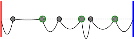
Figure 1: Sketch of a diatomic hard-point chain. Different radii are suggestive of different masses of particles that are assumed to be point-like.

Both types of collisions are described by the same updating rule for the velocities $u_{i}=\dot{x}_{i}$,

$$u_{i}^{\prime}=\frac{m_{i}-m_{i+1}}{m_{i}+m_{i+1}}u_{i}+\frac{2m_{i+1}}{m_{i}+m_{i+1}}u_{i+1}\quad,\quad u_{i+1}^{\prime}=\frac{2m_{i}}{m_{i}+m_{i+1}}u_{i}-\frac{m_{i}-m_{i+1}}{m_{i}+m_{i+1}}u_{i+1},$$ (2)

We consider the case of alternating masses, whose ratio is denoted by $r$, i.e. $m_{i}=m$ for even $i$ and $m_{i}=rm$ , otherwise. This choice is dictated by the need to break the integrability of the model that holds for $r=1$. The particles are confined inside a “box” of length $L$. We consider both periodic boundary conditions

$$x_{n+N}\;=\;x_{n}\,+\,L\quad.$$ (3)

and fixed boundary conditions,

$$x_{1}\;=\;0\qquad x_{N}\;=\;L$$ (4)

Accordingly, the specific volume $\ell=L/N$ is a state variable to be considered together with the specific energy (energy per particle) $e=\sum_{i}m_{i}u^{2}_{i}/2N$.

As it is well known, the thermodynamics of models like ours can be solved exactly (see e.g. Bis ). In particular, the partition function and the equation of state in the $P-T$ ensemble is

$$Z=\prod_{j=1}^{N}\int_{-\infty}^{\infty}dp_{j}\int_{0}^{a}dx_{1}\int_{x_{1}}^{x_{1}+a}dx_{2}...\int_{x_{N-1}}^{x_{N-1}+a}dx_{N}\,\exp[-\beta\sum_{i}\frac{p_{i}}{2m_{i}}-Px_{N}]$$ (5)

where $p_{i}=m_{i}u_{i}$ are the conjugate momenta. Introducing the new variables $\xi_{i}=x_{i+1}-x_{i}$ we find, after some manipulations

$$Z=\lambda^{-N}\left[\int_{0}^{a}d\xi\exp(-\beta P\xi)\right]^{N}=\left[\frac{1}{\lambda\beta P}(1-\exp(-\beta Pa))\right]^{N}$$ (6)

where $\lambda$ is the De Broglie wavelength. The equation of state is given by

$$L=-\frac{\partial\ln Z}{\partial(\beta P)}=N\left[\frac{1}{\beta P}-\frac{a}{\exp(\beta Pa)-1}\right]$$ (7)

This equation is shown in Fig. (2) for $a=1$. For convenience we report the specific volume $\ell$ as a function of $\beta P$. Note that for large $a$ values, the equation of state is the same for an HPG (red line) i.e. the one of an ideal gas in 1D. As a check of our codes (see below) we also computed some state parameters by fixing $\ell$ (namely the box length) and evaluating the pressure as the average exchanged momentum between neighbouring particles.

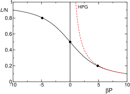
Figure 2: Equation of state of the hard-point chain: the solid line is the analytic expression of eq.7, points are obtained from numerical simulations with $e=1$.

Before discussing the results, let us briefly describe the simulation procedure. Models like the one we are dealing with are particularly suitable for numerical computation as they do not require integration of nonlinear differential equations. Indeed, the dynamics amounts simply to evaluating successive collision times and updating the velocities according to Eqs. (2). The only errors are those due to machine round-off. Moreover, the simulation can be made very efficient resorting to fast updating algorithms. The fact that the $x_{i}$ contribute only indirectly to the evolution, by determining the collision times together with the conservation of the particle ordering along the chain, allows simulating the dynamics with an event driven algorithm that exploits the heap structure of the future collision times grass .

Without loss of generality, we can fix $m=1$ and $a=1$. Most runs have been performed for a mass ratio $r=2$ and for an energy per particle $e=1$, which corresponds to $\beta^{-1}=k_{B}T=2$. Moreover, we have chosen to work with two representative values of the specific volume, namely $\ell=0.2$ and $\ell=0.5$. In the former case, the particles hardly feel the barrier at relative distance $1$, mainly interact only through standard collision. In this regime, the hard–point chain behaves like a gas and is indeed practically equivalent to the HPG. On the contrary, for $\ell=0.5$, the two types of collisions are equally probable, so that the pressure is zero.

3 Diffusion of perturbations

In the spirit of linear response theory forster , transport coefficients can be determined by looking at the way a statistical system reacts to small perturbations (external forces). For heat conductivity, one can directly follow the evolution of an initially localized energy perturbation $\triangle e(x,t)$ helfand . If the perturbation is weak enough for the system to be locally in thermodynamic equilibrium, a reasonable measure of the local temperature field $\triangle T(x,t)$ is $\triangle e(x,t)=C_{P}\triangle T(x,t)$, where $C_{P}$ is the heat capacity per unit length at constant pressure. Thus, by measuring the spreading of the perturbation field, one can estimate how heat propagates through the system helfand . A standard diffusive process is the indication of a normal heat conductivity.

In general, quantities like $\triangle e(x,t)$ are determined by all particles contained in a small box around the spatial location $x$. If, like in our 1D model, particles cannot cross each other, it is more practical to identify $x$ as the average position $i\ell$ of the $i$-th particle. To some extent, this amounts to interpreting the model as a lattice system. Of course, nothing changes in the underlying physics, provided that one consistently adopts the same interpretation throughout. Moreover, since we are mainly interested in the long–time and large–distances behaviours this should not be very relevant, anyhow.

With the above remark in mind, we consider a system at equilibrium with an energy $e_{0}$ per particle and perturb it by increasing by some preassigned $\Delta e$ the energy of a subset of adjacent particles. Let $e(x,t)$ be the energy profile evolving from such a perturbed initial condition. We then ask how the perturbation

$$f(x,t)=\langle e(x,t)-e_{0}\rangle$$ (8)

behaves in time and space. The angular brackets denote an ensemble average over independent trajectories. Because of energy conservation, $\sum_{i}f(i\ell,t)=\Delta e$ at all times, so that $f$ can be interpreted as a probability density (provided that it is also positive-defined and normalized).

At sufficiently long times, one expects that $f(x,t)$ scales as

$$f(x,t)=t^{-\gamma}G(x/t^{\gamma})\qquad\mbox{for $|x|<\tilde{v}t$}.$$ (9)

for some finite velocity $\tilde{v}$.

A sufficiently general framework where the above scaling behaviour is indeed observed is that of Levy walks, where $f(x,t)$ is the probability density of finding a particle whose kinetics is defined as follows. The particle moves balistically in between successive “collisions” whose time separation is distributed according to a power law, $\psi(t)\propto t^{-\mu-1}$, $\mu>0$, while its velocity is chosen from a symmetric distribution $\Psi(v)$. By assuming a $\delta$-like distribution ($\Psi(v)=(\delta(v-\tilde{v})+\delta(v+\tilde{v}))/2$), the propagator $P(x,t)$ (the probability distribution function to find in $x$ at time $t$, a particle initially localized at $x=0$) can be written as $P(x,t)=P_{L}(x,t)+t^{1-\mu}[\delta(x-\tilde{v}t)+\delta(x-\tilde{v}t)]$ where blumen

$$P_{L}(x,t)\propto\begin{cases}\begin{array}[]{ll}t^{-1/\mu}\,\exp\left[-(\eta x/t^{1/\mu})^{2}\right]&|x|\lesssim t^{1/\mu}\\ t\,x^{-\mu-1}&t^{1/\mu}\lesssim|x|<\tilde{v}t\\ 0&|x|>\tilde{v}t\end{array}\end{cases}$$ (10)

Smoother, choices of the velocity distribution $\Psi(v)$ lead to different broader side-peaks, but do not affect the shape and the scaling behaviour of the bulk contribution $P_{L}(x,t)$ which scales as predicted in Eq. (9) with the exponent $\gamma=1/\mu$. Notice also that the two further parameters $\tilde{v}$ and $\eta$ can be scaled out by using proper units of measure for the time and space variables. Nevertheless, we shall see in the following that they can carry some useful information when approaching a transition point.

From the evolution of the perturbation profile, it is possible to infer the growth rate $\alpha$ of the thermal conductivity (see Eq. (1)). In fact, in Ref. klaft , it has been found that $\alpha$, the scaling behaviour of the mean square displacement ($\sigma^{2}(t)=\sum_{i}i^{2}f(x=i\ell,t)\,\propto\,t^{\beta}$ and $\gamma$ are linked by the following relationships, )

$$\alpha\;=\;\beta\;-\;1\;=\;2\;-\;\frac{1}{\gamma}.$$ (11)

In particular, we see that the case $\gamma=1/2$ corresponds to normal diffusion ($\beta=1$) and to a normal conductivity ($\alpha=0$). On the other hand, $\gamma=1$ corresponds to a ballistic motion ($\beta=2$) and to a linear divergence of the conductivity ($\alpha=1$).

3.1 Infinitesimal perturbations

With reference to 1D systems, it is convenient to introduce the variable $\tilde{u}_{i}=\sqrt{m_{i}}u_{i}$ and express the perturbed trajectory as $\tilde{u}_{i}^{p}=\tilde{u}_{i}^{0}+\delta_{i}$, where $\tilde{u}_{i}^{0}(t)$ is an equilibrium trajectory. Since in gas-like systems there is only the kinetic contribution to the energy, Eq. (8) can be written as

$$f(x=i\ell,t)=\langle(\tilde{u}_{i}^{p})^{2}\rangle-\langle(\tilde{u}_{i}^{0})^{2}\rangle=\langle\delta_{i}^{2}\rangle+2\langle\tilde{u}_{i}^{0}\delta_{i}\rangle.$$ (12)

In the limit of infinitesimal perturbations, $\delta_{i}$ follows the tangent space dynamics, i.e. the equation of motion linearized around a reference trajectory. For the hard-point chain this is formally equivalent to that in real space, since the dynamical equations are piecewise linear (the transformations (2) describing the elastic collisions are indeed linear). Accordingly, the energy conservation in real space transforms itself into the conservation of the Euclidean norm $Q=\sum_{i}f(i,t)=\sum_{i}\delta_{i}^{2}(t)$ of a generic perturbation. This, in turn, implies that hard-point systems are not chaotic in the usual sense of the word (all Lyapunov exponents are equal to 0). Moreover, it is reasonable to conjecture (and we have verified numerically) that the dynamics in tangent space is uncorrelated with that in real space, i.e. $\langle\tilde{u}_{i}^{0}\delta_{i}\rangle=0$. As a result, the energy diffusion can be studied by simply looking at the spreading of infinitesimal perturbations

$$f(x=i\ell,t)=\langle\delta_{i}^{2}\rangle$$ (13)

This approach has the advantage of dealing with positive-defined quantities $\delta_{i}^{2}$ and thus allows getting rid of the strong fluctuations affecting positive/negative variables. It is important to notice that this is possible precisely because of the lack of standard deterministic chaos: in chaotic systems, perturbations would exhibit an exponential growth, which can be cancelled only after averaging over an unthinkable number of realizations.

We have first computed $f(x,t)$ for the hard–point chain with an average interparticle distance (specific volume) $\ell=0.2$, a value sufficiently small to expect a perfect agreement with the behaviour of the HPG. In fact, in Fig. 3, we see that $\gamma=0.6$ leads to a very good data collapse in the central region (the side peaks obviously move away, as their position grows linearly in time).

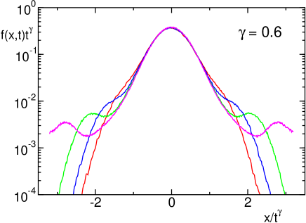
Figure 3: Rescaled perturbation profiles, for the evolution in the tangent space for $N=2045$ and $\gamma=0.6$, at $t=40$, 80, 160, 320 for $\ell=0.2$. The profiles have been obtained by averaging over $10^{4}$ realizations.

These results confirm the behaviour of the HPG described in Ref. denis , where it was also found a perfect agreement with the scaling function predicted for a Levy walk with $\mu=5/3$ (see Eq. (10)). In fact, the only appreciable difference with the theoretical prediction, the broad secondary peaks exhibited by $f(x,t)$, disappears as soon as the $\delta$-Dirac distribution for ${\cal P}(v)$ is replaced by a Gaussian distribution with a suitable width.

Upon increasing the specific volume $\ell$, the effect of finite–distance collisions (that are the novel ingredient of our model) becomes increasingly important. One may thus wonder whether the Levy walk scaling  (10) still describes the perturbation dynamics. To answer this, in Fig. 4, we have plotted the logarithmic derivative

$$\gamma_{eff}=-\frac{d\log f(0,t)}{d\log t}$$ (14)

of the maximum height for two values of the specific volume. For $\ell=0.3$ $\gamma_{eff}$ remains close to $0.6$, though slightly smaller. As it is implausible that the asymptotic value of $\gamma$ depends smoothly on any parameter, we attribute the deviations to finite-size corrections. On the other hand, the deviations from 0.6 observed for $\ell=0.5$ are much stronger: the vicinity of $\gamma_{eff}$ to 1/2 is strongly suggestive of a normal diffusion.

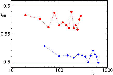
Figure 4: The effective exponent $\gamma_{eff}$, Eq.(14), versus time for two different specific volumes: $\ell=0.3$ (circles) and $\ell=0.5$ (diamonds), $N=2045$

In order to further clarify the dependence on the specific volume, we have plotted in Fig. 5 the profiles corresponding to three different specific volumes. The $x$ axis is scaled so as to yield a unit variance. The good overlap among the various profiles confirms that all cases where the pressure differs from zero exhibit the same universal behavior (the different position of the side peaks reflects simply the different timing and the different ballistic velocities in the three cases).

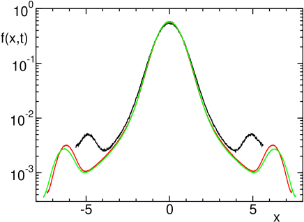
Figure 5: The rescaled profiles for $\ell=0.2$ (at time $t=160$), $\ell=0.3$ ($t=280$), and $\ell=0.4$ ($t=580$). In each case $x$ and $f$ are scaled to yield a unit variance and unit area.

This is to be complemented by the observation that the perturbation profile exhibits, in the zero-pressure limit a clearly different behaviour (see Fig. 6 where the profiles are scaled according to $\gamma=1/2$). No side peaks are present in this case and the bulk appears to convergence towards a Gaussian profile (see the dashed curve, added for reference).

Altogether, all these results suggest that the zero-pressure case is singular and belongs to a different universality class as expected from the mode-coupling theory. This is further confirmed by the behaviour of the parameter $\eta$ (see Eq. (10)) . A convenient way to define $\eta$ is by scaling $x$ in such a way that the variance of $f(x/t^{\gamma})t^{\gamma}$ is equal to 1. As a result, we find that $\eta(\ell)$ diverges, while approaching $\ell=1/2$. A fit of the few available points is consistent with an inverse square root divergence, but many factors prevent considering this prediction too seriously.

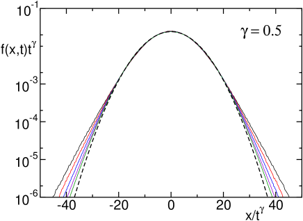
Figure 6: Rescaled perturbation profiles for $\ell=0.5$, $N=2045$, at $t=50$, 100, 200, 400. and 750. The profiles have been obtained by averaging over $10^{4}$ realizations. The dashed line corresponds to a Gaussian.

Although this result is a clear confirmation that the zero-pressure case corresponds to a different universality class, it poses a problem, since normal diffusion should correspond to normal conductivity. This prediction is totally in contrast with both the numerical results for the FPU-$\beta$ system and the solution of the mode-coupling equations which instead suggest a stronger divergence for the conductivity.

3.2 Finite perturbations

In order to understand the puzzling behavior of infinitesimal perturbations, it is worth exploring the dynamics of finite rather than infinitesimal perturbations. In fact, the signature of “stable chaos”, a type of irregular behaviour found in linearly stable coupled map lattices, is precisely the different propagation rate for finite and infinitesimal perturbations PT . Moreover, since it was already argued in Ref. denis that the HPG might be a Hamiltonian model exhibiting stable chaos, it is not unreasonable to expect a different behaviour for the two classes of perturbations.

With reference to Eq. (12), we follow pairs of trajectories $(\tilde{u}_{i}^{0}(t),\tilde{u}_{i}^{p}(t))$, where the first element is a typical unperturbed equilibrium configuration and the second element is obtained from the first one by adding a given amount of energy in the three sites around the origin. We then study the evolution of the perturbation by computing the ensemble average of the instantaneous local distance $\Delta(x,t)=\langle(\tilde{u}_{i}^{p}(t)-\tilde{u}_{i}^{0}(t)^{2}\rangle$ and the ensemble average of the energy difference $\Delta e(x,t)=\langle(\tilde{u}_{i}^{p}(t))^{2}\rangle-\langle(\tilde{u}_{i}^{0}(t))^{2}\rangle$.

From the results reported in Fig. 7, the central peaks show a good overlap for $\gamma=0.55$. Considering the shorter time scales with respect to those ones achieved in the corresponding tangent-space simulations, the deviation from $0.6$ cannot be taken as an indication of a different scaling behaviour. A substantial difference is instead found by comparing the velocity of the side peaks which is definitely larger in this second context (see the next section for a detailed discussion). The too short time scales prevent a quantitative comparison with the predictions of the Levy walk model: in fact the central peak should decay by another order of magnitude to appreciate deviations from the Gaussian behaviour.

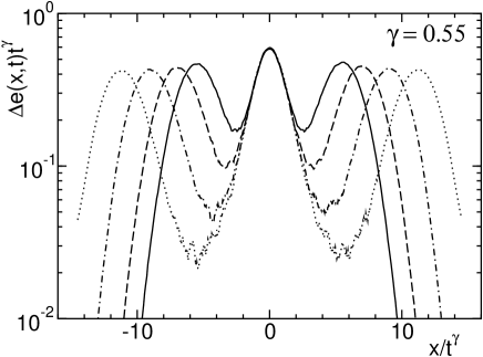
Figure 7: Energy perturbation profiles for an energy density $e=1$, at $t=5$, 10, 20, and 35 ($N=2045$), for $\ell=0.2$. The profiles have been obtained by averaging over $10^{4}$ realizations.

In Fig. 8 we plot the amplitude of the perturbation itself. The propagation velocity is estimated by determining the half-height position of the front (see the horizontal dashed line) at different times. The velocity $c_{fa}$ turns out to coincide with that of the side peaks in the set-up of Fig. 7.

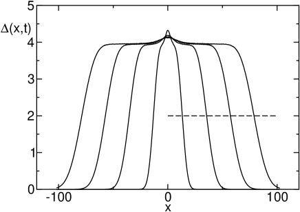
Figure 8: Propagation of finite amplitude perturbations for $N=2045$, energy density $e=1$ and $\ell=0.2$. The profiles have been obtained by averaging over $10^{4}$ realizations. Different curves are at times $t=5$, 10, 20 and 35 respectively.

Finally, we have studied the case $\ell=0.5$. As it can be seen in Fig. 9, in the available time range we do not appreciate any difference with respect to the previous non-zero pressure case. Moreover, in agreement with tangent space results, the side peaks are basically absent. Altogether, fluctuations in real space are so strong that it is almost impossible to extract any useful information, apart from the velocity of the perturbations themselves, that is the only observable unambiguously different with respect to that of infinitesimal perturbations.

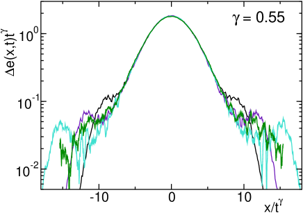
Figure 9: Rescaled energy perturbation profiles for an energy density $e=1$, at $t$=12, 24, 48, 96 ($N=2045$), for $\ell=0.5$, $\gamma$=0.55. The profiles have been obtained by averaging over $10^{4}$ realizations.

4 Ballistic phenomena

In the previous section we have encountered two different velocities for the propagation of infinitesimal and finite perturbations. From a thermodynamic point of view, there exist two further velocities: the adiabatic $c_{ad}$ and the isothermal $c_{is}$ sound velocity, which are defined respectively as

$$c_{ad}^{2}=\Big{(}\frac{\partial P}{\partial\rho}\Big{)}_{S}\qquad\qquad c_{is}^{2}=\Big{(}\frac{\partial P}{\partial\rho}\Big{)}_{T}$$ (15)

where $\rho$ is the mass density. They are related by

$$c_{ad}^{2}\;=\;\frac{C_{P}}{C_{V}}\;c_{is}^{2}$$ (16)

where $C_{P}$ and $C_{V}$ are the constant-pressure and constant-volume specific heats.

From the equation of state (5), we can determine both velocities for the hard-point chain. They are reported in Fig. 10 versus the specific volume. For $\ell\to 0$, the hard-point chain reduces to the HPG model. In this limit, a simple expression can be obtained for the two velocities. The equation of state reduces to

$$PL\;=\;k_{B}NT\;=\;\frac{2\rho}{1+r}\frac{k_{B}T}{m}$$ (17)

where $\rho=m(1+r)L/2N$. From Eq. (15) we obtain,

$$c_{is}^{2}=\frac{2k_{B}T}{(1+r)m}\qquad\qquad c_{ad}^{2}=3\;c_{is}^{2}$$ (18)

because $C_{P}/C_{V}=3$ in the HPG. By inserting the parameters used in the the numerical simulations we obtain $c_{is}=1.154$ and $c_{ad}=2$ for $r=2$, and $c_{is}=1$, $c_{ad}=1.722$ for $r=3$.

We can now compare all such velocities. From the position of the side peaks for different specific volumes, we obtain the tangent–space velocity $c_{ta}$ (circles in Fig. 10). In the HPG limit, $c_{ta}$ coincides with $c_{is}$ (we have checked that this holds true also for different mass ratios). However, upon increasing the specific volume $c_{is}$ increases, while $c_{ta}$ decreases and vanishes when $\ell$ approaches 0.5. Besides confirming the peculiarity of the zero-pressure case, these simulations reveal that $c_{ta}$ differs from both thermodynamical velocities.

Furthermore, we have determined the velocity $c_{fa}$ of finite-amplitude perturbations (diamonds in Fig. 10), finding that it is close to, though slightly larger than $c_{ad}$ . The difference is larger than the statistical fluctuations, but we cannot exclude that this is due to systematic deviations that vanish at longer times. We have verified that $c_{fa}$ agrees also with the velocity estimated from the dispersion of long-wavelength Fourier modes.

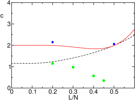
Figure 10: Thermodynamic velocities versus the specific volume $\ell=L/N$ for the hard point chain. Solid and dashes curves correspond to the adiabatic and isothermal velocity, respectively. The solid circles correspond to the propagation velocity as determined from the behaviour of infinitesimal perturbations, while the diamonds correspond to the velocity of finite amplitude perturbations.

From the dynamical point of view, the most important observation is however that $c_{fa}$ is definitely larger than $c_{ta}$. This inequality is the typical signature of “stable chaos”. In order to strenghten this conclusion we show in Fig. 11 another typical feature of stable chaos, i.e. that self-sustained irregular behaviour is accompanied by the presence of discontinuities in phase-space dynamics. By discontinuiy, we mean a codimension one manifold across which an infinitesimal difference in the initial conditions is amplified to a finite value in a finite time . In Fig. 11, we show that this indeed occurs in the HPG in the vicinity of a three–body collision. By shifting the central particle to the right, one discontinuously passes from the sequence of collisions depicted in panel a to the sequence depicted in panel b. Since the effects of the collisions do not commute, one has a discontinuous change in the outcoming velocities, while passing through the configuration which yields the three body collision. In the vicinity of such discontinuities, small but finite perturbations are suddenly amplified and this provides a mechanism for sustaining irregular behavior in the absence of an exponential amplification of infinitesimal differences.

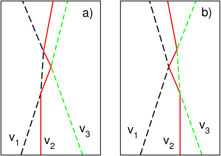
Figure 11: The evolution of three neighbouring particles in the vicinity of a three body collisions.

5 The energy current

In view of the difficulties encountered in extracting the scaling behavior of thermal conductivity from direct energy diffusion simulation, we now turn our attention to the fluctuations of the total heat flux. Our past experience with other 1D models in fact suggests that this observable is much more reliable since the fluctuations due to the spatial dependence are integrated out.

In order to properly treat hard-point chains, it is necessary to implement the general microscopic definition of the heat flux LLP03

$$j_{i}=\frac{1}{2}(x_{i+1}-x_{i})(u_{i+1}+u_{i})F(x_{i+1}-x_{i})+\frac{1}{2}m_{i}\dot{x}_{i}^{3}\equiv j_{i}^{(1)}+j_{i}^{(2)}$$ (19)

where $F$ denotes the force exerted by the $i$–th particle on its right neighbor. In the HPG, only the second term matter, since interactions occur only when the relative distance between the neighbouring particles $x_{i+1}-x_{i}$ vanishes. On the contrary, in the hard-point chain, “collisions” occur also at the distance $a$. However, since the force is singular, one cannot implement the definition (19) as it stands. By defining the force between two particles as the momentum difference induced by a collision, $j_{i}^{(1)}$ can be written as the kinetic energy variation times the actual distance $a$, i.e., $j_{i}^{(1)}=am_{i}(u_{i}^{{}^{\prime}2}-u_{i}^{2})/2$ divided by a suitable time-interval $\Delta t$. In order to get rid of the microscopic fluctuations, it is necessary to consider a sufficiently long $\Delta t$, so as to include a large number of collisions. Since the number of collisions is proportional to the system size, it is only in long systems that fluctuations can be removed without spoiling the slow dynamics of the heat flux. By fixing $\Delta t=1$ in our arbitrary units, it is sufficient to simulate a few hundreds of particles.

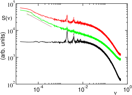
Figure 12: Power spectrum of the heat flux for energy density $e=1$ and specific volume $\ell=0.5$. Solid and dashed lines refer to $N=2045$ and $N=1021$ respectively. From bottom to top: the contribution due to $j^{(2)}$, $j^{(1)}$ (see Eq. (19), and their sum. Power spectrum have been obtained by averaging over $10^{4}$ realizations.

Besides computing the power spectrum $S(\nu)$ of the total flux, we have determined the power spectrum of the two separate contributions $j^{(1)}$ and $j^{(2)}$ for $\ell=0.5$. The $j^{(2)}$ contribution, which exhibits $\nu^{-1/3}$ power-law divergence in the HPG, here appears to saturate (see the lowest solid curve in Fig. 12). From the comparison with the spectrum obtained for a shorter chain length (see the dashed curve), it is clear that the saturation is not a finite-size effect. Accordingly, one might be tempted to conclude that the zero-pressure case is characterized by a normal conductivity as also suggested by the simulation performed in tangent space. However, the spectrum of the other contribution $j^{(1)}$, shows that this is not such conclusion is incorrect. In fact, the middle solid curve exhibits a low-frequency divergence which is terminated by a finite-size saturation (as revelead by looking at the spectra corresponding to two different chain lengths). A power-law fit within the central frequency range (i.e. away from the saturation region) yields an exponent around 0.45 (see the straigh segment, shifted for the sake of clarity). This value is not only definetely larger than the 1/3 value predicted for nonzero pressure, but it is also fairly close to the results found for the FPU-$\beta$ model LLP03b . Although we cannot claim a quantitative confirmation of the 1/2 prediction of mode-coupling theory, the conjecture that zero-pressure systems do belong to a different universality class is further strengthened.

On the other hand, one should not forget that the heat flux definition requires summing the two contributions we have separately analysed. By doing so, not unexpectedly, the resulting power spectrum exhibits an intermediate behaviour (see the top curve in Fig. 12). It is reasonable to conjecture that the resulting slower convergence is a finite-size correction due to the strong constant background due to the $j^{(2)}$ contribution, but it is also honest to admit that these results altogether confirm the difficulty of extracting reliable estimates in zero-pressure systems.

6 Adding internal degrees of freedom

For the sake of completeness, we have explored another variant of the HPG that is obtained by introducing an additional degree of freedom to each particle in the original model. As it is sketched in Fig. 13, particles are replaced by infinitesimally thin disks, which can rotate along the $x$ axis and thereby possess an angular velocity as well as an angular momentum that we denote with $\zeta_{i}$. Like in the original HPG model, collisions do occur whenever the longitudinal position of two neighbouring particles coincides and the dynamics is determined by the corresponding collision rules. Besides linear momentum $P_{i}$ and energy $E_{i}$, there is another conserved quantity, namely angular momentum $Z_{i}$. For the sake of simplicity, we consider an equal-disk gas, while the units of measure are chosen in such a way that both the mass and the momentum of inertia are set equal to 1. Altogether, the quantities

$$P_{i} = p_{i}+p_{i+1}$$

$$Z_{i} = \zeta_{i}+\zeta_{i+1}$$ (20)

$$E_{i} = p^{2}_{i}+\zeta^{2}_{i}+p^{2}_{i+1}+\zeta^{2}_{i+1}$$ (21)

are left invariant by the collision. One can easily verify that the following transformations satisfy the above constraints,

$$p^{\prime}_{i} = p_{i}\sin^{2}\phi+p_{i+1}\cos^{2}\phi+(\zeta_{i+1}-\zeta_{i})\sin\phi\cos\phi$$

$$p^{\prime}_{i+1} = p_{i}\cos^{2}\phi+p_{i+1}\sin^{2}\phi-(\zeta_{i+1}-\zeta_{i})\sin\phi\cos\phi$$ (22)

$$\zeta^{\prime}_{i} = \zeta_{i}\cos^{2}\phi+\zeta_{i+1}\sin^{2}\phi+(p_{i+1}-p_{i})\sin\phi\cos\phi$$

$$\zeta^{\prime}_{i+1} = \zeta_{i}\sin^{2}\phi+\zeta_{i+1}\cos^{2}\phi-(p_{i+1}-p_{i})\sin\phi\cos\phi$$

where $\phi$ is a free parameter. One might determine a deterministic updating rule for $\phi$ by assuming a specific interaction Hamiltonian during the collision. For the sake of simplicity, we have preferred to randomly extract $\phi$ according to a flat distribution restricted to the angles which guarantee that the outgoing velocities change direction (to avoid particle crossing).

Although this model has been developed by assuming that $\zeta_{i}$ is an angular momentum, it equally applies to the case where $\zeta_{i}$ is a linear momentum, like for a chain embedded in a planar geometry with transverse periodic boundary conditions. Actually, this latter interpretation would make the model almost identical to that one studied in DN03 .

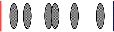
Figure 13: Sketch of the hard disk model

Like before, we have studied the evolution of an energy packet in tangent space, $f(x,t)=\delta p^{2}_{i}(t)+\delta\zeta^{2}_{i}(t)$, having the care of referring to the same sequence of $\phi$ values in the real as well as in tangent space.

The quantitative result of numerical studies are very similar to the diatomic HPG denis and to the hard-point chain model with $\ell=0.2$. More precisely, the evolution in the tangent space is in a good agreement with the Levy–walk model with the same scaling exponent $\gamma=0.6$ (Fig. 14).

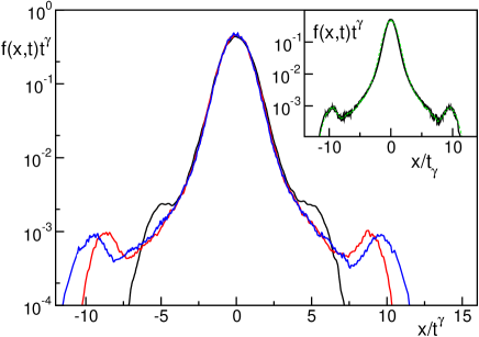
Figure 14: Rescaled perturbation profiles, for the evolution in the tangent space, at $t=80,160,240$ for the generalized HPG, Eqs.(22). The profiles have been obtained by averaging over $10^{4}$ realizations. In the inset, the profile at $t=160$ (solid line) is compared with the propagators of a Levy walk for an exponent $\mu=5/3$ with a Gaussian distribution with average equal to 1 and rms 0.0347)(dashed line).

Numerical value of the velocity propagation is consistent with the isothermal sound velocity of the hard-point chain model with $\ell=0.2$ and equal masses.

7 Conclusions and open problems

In this paper we have seen that the hard-point chain model allows extending the same approaches developed for the hard-point gas to a system, where the pressure can be tuned from positive to negative values. We have restricted our analysis to nonnegative pressure values, because the evolution for negative pressures is symmetrically related to that for positive values (see, e.g., the equation of state as plotted in Fig. 2). Although, the various numerical techniques have confirmed the difficulties in extracting reliable estimates of scaling rate, we have been able to convincingly show that the zero-pressure case belongs to a different universality class. The most compelling evidence is arising from the tangent space evolution: (i) the scaling exponent $\gamma$ is close to 1/2 instead of 3/5 as for the hard point gas; (ii) the velocity $c_{ta}$ goes to zero.

Another general observation follows from the different propagation velocity exhibited by finite and infinitesimal perturbations. We interpret this fact as an indication that the behavior of hard-point chains is an instance of “stable chaos”, i.e. an irregular dynamical regime sustained by discontinuities in phase-space rather than by the exponential amplification.

Besides these two general comments, all conclusions about the scaling behaviour require further checks and a more careful analysis (if doable at all). For instance, although it is quite reasonable to assume that the scaling rate $\gamma$ is always equal to $3/5$ whenever the pressure is different from 0, it should be verified that the systematic deviations observed for the specific volume $\ell=0.3$ decay when going to longer times.

On the other hand, the difficulties encountered while performing simulations with finite amplitude perturbations indicate that there is little room to make progress, by adopting this approach. In this sense, it is perhaps a better idea looking directly at the behaviour of the correlation function of the energy density zhao ,

$$C_{e}(x,t)=\langle\delta e(y,\tau)\delta e(x+y,t+\tau)\rangle\quad,$$ (23)

where the angular brackets denote a spatial as well temporal average. At $t=0$, the correlation function $C_{e}(x,0)$ is a $\delta$ function in space. Moreover, in the microcanonical ensemble, energy conservation implies that the area $\int dxC_{e}(x,t)$ is constant at all times. By therefore assuming that $C_{e}(x,t)$ is normalizet to have unit area, its behaviour is formally equivalent to that a diffusing probability distribution. This observation has led Zhao to determine the scaling behaviour of the heat conductivity from the growth rate of the variance of $C_{e}(x,t)$ zhao . As the determination of the variance is troubled by the fluctuating tails, it is preferrable to proceed like in the previous sections, by looking at the decay of the maximum $C_{e}(0,t)$ that is statistically more reliable. For the sake of providing a concrete example of such an approach, we performed a microcanonical simulations of an FPU-$\beta$ chain in a lattice of 2048 particles. The correlations $C_{e}(x,t)$ for different times, are reported in Fig. 15. They have been rescaled by choosing $\gamma=0.642$, a value that has been determined from a best fit of the maximum of the correlation function. From the Levy-walk machinery, it follows that $\alpha=2-1/\gamma\approx 0.44$. This value is significantly different from 1/3 and definitely confirms that zero-pressure systems do belong to a different universality class. On the other hand $0.44$ is still not so close to the mode-coupling prediction (1/2) and thus confirms once more the presence of strong finite-size corrections which certainly need be understood before making conclusive claims.

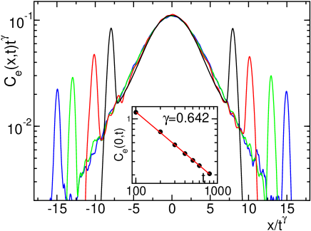
Figure 15: Rescaled energy correlation function for the FPU-$\beta$ model, for an energy density $e=1$. The different profiles, which correspond to times $t=100$, 200, 400, and 600, have been obtained by averaging over $10^{4}$ realizations. In the inset the decay of the maximum is reported versus time together with a best power-law fit.

References

- (1) K. Hahn, J. Kärger, and V. Kukla, Phys. Rev. Lett. 76, 2762 (1996).
- (2) Y. Pomeau, R. Résibois, Phys. Rep. 19 (1975) 63.
- (3) O. Narayan, S. Ramaswamy, Phys. Rev. Lett. 89, 200601 (2002).
- (4) S. Pal, G. Srinivas, S. Bhattacharyya and B. Bagchi, J. Chem. Phys. 116 5941 (2002).
- (5) S. Lepri, R. Livi, A. Politi, Phys. Rev. Lett. 78, 1896 (1997); Europhys. Lett. 43, 271 (1998).
- (6) S. Lepri, R. Livi, A. Politi, Phys. Rep. 377, 1 (2003).
- (7) S. Lepri, R. Livi, A. Politi, Chaos 15, 015118 (2005)
- (8) D. D’Humieres, P. Lallemand, Y. Qian, C. R. Acad. Sci. Paris 308, serie II 585(1989).
- (9) M. Bishop, J. Stat. Phys 29 (3), 623 (1982).
- (10) S. Lepri, P. Sandri, A. Politi Eur. Phys. J. B 47, 549 (2005).
- (11) J. Scheipers, W. Schirmacher, Z. Phys. B 103 547 (1997).
- (12) S. Lepri, Phys. Rev. E 58 7165 (1998).
- (13) L. Delfini, S. Lepri, R. Livi and A. Politi, Phys. Rev. E 73, 060201(R) (2006).
- (14) G. R. Lee-Dadswell, B. G. Nickel, and C. G. Gray, Phys. Rev. E 72 031202 (2005).
- (15) L. Delfini, S. Lepri, R. Livi and A. Politi, cond-mat/0611278.
- (16) P. Cipriani, S. Denisov and A. Politi, Phys. Rev. Lett. 94, 244301 (2005).
- (17) S. Lepri, R. Livi, A. Politi, Phys. Rev. E 68 067102 (2003).
- (18) G. Casati, Found. Phys. 16 51 (1986).
- (19) T. Hatano, Phys. Rev. E 59, R1 (1999).
- (20) A. Dhar, Phys. Rev. Lett. 86 3554 (2001).
- (21) P. Grassberger, W. Nadler, L. Yang, Phys. Rev. Lett. 89, 180601 (2002).
- (22) G. Casati and T. Prosen, Phys. Rev. E 67, 015203(R) (2003).
- (23) P.I. Hurtado, Phys. Rev. Lett. 96, 010601 (2006).
- (24) A. V. Savin, G. P. Tsironis and A. V. Zolotaryuk, Phys. Rev. Lett., 85, 154301 (2002).
- (25) A. Politi, R. Livi, G.L. Oppo and R. Kapral, Europhys. Lett. 22, 571 (1993).
- (26) M. Bishop, M.A. Boonstra, Am. J. Phys. 51 (6) 564 (1983).
- (27) D. Forster, Hydrodynamic Fluctuations, Broken symmetry and Correlation Functions (W. A. Benjamin, Reading, 1975).
- (28) E. Helfand, Phys. Rev. 119, 1 (1960).
- (29) A. Blumen, G. Zumofen, and J. Klafter, Phys. Rev. A 40, 3964 (1989).
- (30) S. Denisov, J. Klafter and M. Urbakh, Phys. Rev. Lett. 91, 194301 (2004).
- (31) A. Politi and A. Torcini, Europhys. Lett. 28, 545 (1994).
- (32) R. Bonaccini and A. Politi, Physica D 103, 362 (1997).
- (33) J.M. Deutsch, O. Narayan, Phys. Rev. E 68 010201 (2003).
- (34) H. Zhao, Phys. Rev. Lett. 96, 140602 (2006).