Binding of holons and spinons in the one-dimensional anisotropic $t$-$J$ model

Abstract

We study the binding of a holon and a spinon in the one-dimensional anisotropic $t$-$J$ model using a Bethe-Salpeter equation approach, exact diagonalization, and density matrix renormalization group methods on chains of up to 128 sites. We find that holon-spinon binding changes dramatically as a function of anisotropy parameter $\alpha=J_{\perp}/J_{z}$: it evolves from an exactly deducible impurity-like result in the Ising limit to an exponentially shallow bound state near the isotropic case. A remarkable agreement between the theory and numerical results suggests that such a change is controlled by the corresponding evolution of the spinon energy spectrum.

In the one-dimensional $t$-$J$ and Hubbard models, spin and charge dynamics are independent, leading to the well-known effect of spin-charge separation: the splitting of the electron (hole) into spinon and holon excitations that carry only spin and only charge, respectively LiebWu . Considerably less is known about interactions among these excitations. Recently, it was shown that in the supersymmetric $t$-$J$ model, spinons and holons attract each other Bernevig , but this does not result in a bound state, indicating that the spinon-holon interaction is non-trivial.

Figure 1: (Color online). A hole in the Ising AF (circle) moved by four sites from origin. The spinon is indicated by the dashed box.

On the other hand, there is a limit in which spinon and holon do form a bound state: the $t$-$J_{z}$ model sorella-1d . Here, the half-filled system is an Ising antiferromagnet (AF). Removing a spin and moving the hole away from origin increases the net magnetic energy by $J_{z}/2$ due to creation of a domain wall in the AF order – an immobile spinon (Fig. 1). Once moved, the hole also carries an AF domain wall and is a free holon with dispersion $\epsilon^{0}_{k}\!=\!-2t\cos k$. Since recombination with the spinon lowers the energy of the system, the holon can be considered as moving freely except at the origin where it is subject to an effective attractive potential $V\!=\!-J_{z}/2$. Clearly, such a potential in 1D always leads to a bound state. The single-hole Green’s function can be found exactly: $G(\omega)\!=\!\left[J_{z}/2\pm\sqrt{\omega^{2}-4t^{2}}\right]^{-1}$. Its lowest pole gives the binding energy of the spinon-holon bound state:

$$\Delta=2t\left(1-\sqrt{1+J^{2}_{z}/16t^{2}}\right),$$ (1)

in which holon is confined in the vicinity of the spinon with the localization length $\ell\!\propto\!\Delta^{-1/2}$. This leads to the question: how does the Ising limit, in which the spin and charge are bound, evolve into the isotropic limit where they separate? This question, together with the expectation that the study of anisotropic model can shed light on the general problem of spinon-holon interactions, motivates this work.

In this Letter we address this problem by a detailed theoretical and numerical study of the anisotropic $t$-$J$ model using the Bethe-Salpeter equation (BSE), exact diagonalization (ED), and density matrix renormalization group (DMRG) dmrg methods on systems of up to 128 sites. Although the binding becomes too weak to be detected numerically near the isotropic limit, we believe that a holon and a spinon form a bound state for any value of anisotropy $\alpha=J_{\perp}/J_{z}$ less than one. Given a remarkable agreement between the theory and numerical results, we argue that the binding is largely controlled by the spinon energy spectrum. Qualitatively, at $\alpha\ll 1$ the holon is confined in the vicinity of the impurity-like spinon, while already for $\alpha\gtrsim 0.5$ the spinon is quasi-relativistic and is only weakly bound to the holon. Such a change in the pairing character results in a dramatic decrease of the binding energy at larger $\alpha$. In addition, using a small-$\alpha$ analysis, we provide insight into the kinematic structure of the spinon-holon interaction that offers a simple explanation for having an attraction but no bound state in the isotropic limit of the model.

Using standard notation, we define a generalization of the 1D $t$-$J$ model, ${\mathcal{H}}=\sum_{i,j}{\mathcal{H}}_{i,j}$, with

$${\mathcal{H}}_{ij}=-t\sum_{\sigma}c^{\dagger}_{i\sigma}c^{\phantom{\dagger}}_{j\sigma}+\frac{J_{z}}{2}\left(S^{z}_{i}S^{z}_{j}+\alpha S^{+}_{i}S^{-}_{j}-\frac{n_{i}n_{j}}{4}\right),$$ (2)

where $i$ and $j=i\pm 1$ are the neighboring sites. This model interpolates between the $t$-$J_{z}$ model ($\alpha=0$) and the isotropic $t$-$J$ model ($\alpha=1$). We set $t=1$.

To obtain the binding energy numerically, we have performed calculations of the ground state energies (GSEs) using both ED and DMRG techniques. While only small system sizes are accessible by ED (up to $L\!=\!23$ sites in our case), it allows us to calculate the lowest energy in each momentum sector (Fig. 2) and is also important in analyzing various finite-size effects. Using DMRG dmrg we have calculated GSEs of systems of up to $L\!=\!128$ sites using periodic boundary conditions (PBCs), which greatly increases the numerical effort required. Up to $m\!=\!1400$ states per block were kept in the finite system method, with corrections applied to the density matrix to accelerate convergence with PBCs singlesite . The binding energy $\Delta$ for the infinite system was obtained using two different extrapolation methods described below. In the range of $\alpha$ where the calculation of $\Delta$ is reliable ($\alpha\!\lesssim\!0.6$), we found excellent agreement between the numerical data from both methods, and theoretical results, based on BSE. A summary of the results for $J_{z}\!=\!4.0$ is presented in Fig. 3; results for other values of $J_{z}$ are qualitatively similar.

Figure 2: Lowest energies $E_{k}\!-\!E_{0}$ vs $k$ in an $L\!=\!21$ chain with (a) zero and (b) one hole, $J_{z}\!=\!4.0$. Solid lines in (a) is the spinon dispersion from BA johnson-excitations-xyz ; in (b) the lines are guides to the eye.

Numerics. For a given $J_{z}$ and $\alpha$, the binding energy is

$$\Delta=E_{p}-E_{s}-E_{h},$$ (3)

where $E_{x}$, $x\!=\!p,s,h$, is the GSE of the $L\!=\!\infty$ chain with the spinon-holon pair, the spinon, and the holon, all relative to GSE of the $XXZ$ chain, respectively. It is well known shiba-ogata-review ; zotos-tbc that the energies of individual spinon and holon can be obtained from GSEs of odd-$L$ periodic chains with no holes and one hole, respectively. The even-$L$ periodic chain with one hole contains the spinon-holon pair. A consistent finite-size definition of $\Delta_{L}$ for even $L$ is:

$$\Delta_{L}=E^{0}_{L}+E^{1}_{L}-\frac{1}{2}\left(E^{0}_{L-1}+E^{0}_{L+1}+E^{1}_{L-1}+E^{1}_{L+1}\right),$$ (4)

where $0$ and $1$ refer to the number of holes. It can be used directly to obtain a sequence of binding energies $\Delta_{L}$ for different $L$, which can then be extrapolated to $L\!=\!\infty$ limit. We will call this approach “method $B$”. An alternative and substantially more precise way to estimate $\Delta_{\infty}$ is: (i) to obtain $E_{x}(L)$ by subtracting the extensive part of energy $\tilde{\varepsilon}_{\alpha}L$ from corresponding GSEs ($\tilde{\varepsilon}_{\alpha}$ is the energy per site of an infinite $XXZ$ chain, known from Bethe-Ansatz (BA) yang-xxz ), (ii) extrapolate $E_{x}(L)$ to the infinite system size, and (iii) use Eq. (3). We will refer to this approach as “method $A$”. In this method we use the exact $L=\infty$ value for the spinon energy $E_{s}$ that is also known from BA johnson-excitations-xyz , thus completely eliminating one of the sources of the finite-size effects.

Method A. One of the problems is the “staggered” behavior of the holon and pair energies vs $L$, meaning that the data must be separated into two branches, defined by whether $L$ for the pair ($L-1$ for the holon) is divisible by 4. We refer to them as “$4$-even” and “$4$-odd” branches, respectively (see also Ref. Bernevig, ). Within each branch energy depends on the size smoothly. We found for both holons and pairs that although one of the branches may exhibit a non-uniform dependence on system size, the other one is always well-behaved, see Fig. 4. Thus, even though we have fewer points in the “good” branch, the quality of extrapolation using it is vastly improved.

In fact, for the holon data, we can further advance this success by doubling the number of points in each branch using the “twisted” boundary conditions (BCs) zotos-tbc . The GS of a holon in an infinite chain is degenerate for $k=0$ and $k=\pi$. For a finite $L$, this degeneracy is lifted: in $4$-even chains $E_{0}$ is shifted up and $E_{\pi}$ is higher in the $4$-odd ones (see Fig. 2). The staggering occurs because the $k$-space of odd-$L$ chains does not contain the $k=\pi$ point. This can be mitigated by flipping the sign of the hopping integral $t$, which shifts the momentum by $\pi$. Thus, we can construct the GSEs for both branches in every odd-$L$ chain by combining the data as follows:

$$\left.\begin{array}[]{l}\text{mod}(L-1,4)=0,t=+1\\ \text{mod}(L-1,4)\not=0,t=-1\end{array}\right\}\ \ 4\text{-even branch}.$$ (5)

The complementary data goes into $4$-odd branch. An example of such reconstruction, along with the extrapolation to the infinite size, is shown in Fig. 4(a).

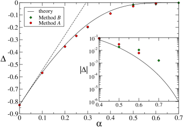
Figure 3: (Color online). Theoretical (lines) and numerical results by method $A$ (circles) and method $B$ (diamonds) for $\Delta$ vs $\alpha$, $J_{z}=4.0$. Inset: $|\Delta|$ for $\alpha\geq 0.4$ on a semi-log plot.

For the spinon-holon pair data, the separation into two branches also allows for a smooth $E$ vs $1/L$ scaling. Further improvement using twisted BCs can be achieved by multiplying $t$ with an a priori unknown $L$-dependent complex phase factor zotos-tbc . While such BCs can be easily handled by ED, our DMRG code requires extensive modifications to support them. Results featuring phase-adjusted data will be presented elsewhere elsewhere .

Branch	$\text{mod}(L,4)$	$\text{sign}(t)$ for $E^{1}_{L-1}$	$\text{sign}(t)$ for $E^{1}_{L+1}$
$B1$	0	-1	+1
$B2$	0	+1	-1
$B3$	2	-1	+1
$B4$	2	+1	-1

Table 1: Subdivision of the numerical data for $\Delta(L)$ into different branches due to finite size effects in method $B$.

Having significantly improved the scaling quality of the available GSE data, we need to choose the functional form for the $E$ vs $1/L$ fit. We find that at not too large $\alpha$ GSEs approach $E_{\infty}$ exponentially fast. Notably, similar exponential convergence of the energy of the finite $XXZ$ chain at large $L$ was derived by Woynarovich and de Vega (WdV) using BA vega-woynar-size-corr . Thus, we attempt to fit both holon and pair data with $E_{L}\!=\!E_{\infty}\!+\!e^{-\lambda L}P_{n}(1/L)$, where $P_{n}(x)$ is a polynomial of order $n$. Remarkably, the values of $\lambda$ we found for holons are in close agreement with WdV ones, so we used them in our holon fits. For pairs there is no such correlation, so we retain $\lambda$’s as free parameters. Example of pair energy extrapolation is shown in Fig. 4(b).

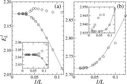
Figure 4: The $4$-even (circles) and $4$-odd (squares) branches for (a) holon and (b) pair energies vs $1/L$. $J_{z}=4.0$ and $\alpha=0.4$ ($\alpha=0.25$, insets). Dashed curves are the fits described in text.

Finally, we are able to obtain high-precision values for the $L\!=\!\infty$ binding energies in the range $0\!\leq\!\alpha\!\leq\!0.5$ using (3). The data for $J_{z}=4.0$ are shown in Fig. 3. By studying the quality of the fits and the variation of $\Delta_{\infty}$ depending on the fit type, we estimate the error to be less than 3% for $\alpha\!=\!0.5$ and negligible for smaller values of $\alpha$. For $\alpha\!>\!0.5$ parameter $\lambda$ drops below $1/L_{max}$, so the corresponding fits become less reliable. For $\alpha\!=\!0.6$ the error is of the order of 10%, and for $\alpha=0.7$ it exceeds $100$%. In principle, our results at larger $\alpha$ can be improved by increasing $L$ while keeping the DMRG precision the same ($\sim\!10^{-4}t$). However, as one can see from the inset in Fig. 3, the binding energy itself diminishes rapidly and it is likely to hit the DMRG accuracy around $\alpha\sim 0.8$.

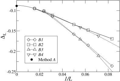
Figure 5: $\Delta_{L}$ data vs $1/L$ in method $B$, $J_{z}=4.0$ and $\alpha=0.4$. Branches are defined in Table 1. Dashed lines are guides to the eye, solid line is the $4$-th order polynomial fit of the $B2$ branch.

Method B. The “direct” extrapolation of $\Delta_{L}$ using Eq. (4) (method $B$), does not rely on prior knowledge of BA results. Thus, it provides an important validity test for the results of method $A$. The $\Delta_{L}$ data is, again, staggered, and has to be separated into the $4$-even and $4$-odd branches. We also have a freedom in choosing the sign of $t$ for the holon energies $E^{1}_{L-1}$ and $E^{1}_{L+1}$. As a result, data splits into four different branches, defined in Table 1. An example of size dependence for different branches is shown in Fig. 5. The best choice, corresponding to the “good” holon branch in method $A$, is branch $B2$. The results of extrapolation of $B2$ data using polynomial fit of maximum order are shown in Fig. 3. They are in close agreement with method $A$. Inspection of the terms in (4) reveals that most significant finite-size effects in method $B$ come from the spinon energies $E^{0}_{L\pm 1}$ (eliminated in method $A$). Even though method $B$ serves as an important validity test, its relative error is always larger than that of method $A$.

Theory. Generally, the binding energy in 1D should scale as $-V^{2}m$, where $V$ is the interaction and $m$ is a particle mass. For the Ising limit this estimate gives $\Delta\!\sim\!-J_{z}^{2}/t$ in agreement with the exact answer (1). To extend our approach to the finite $\alpha$, we use BSE formalism LL in which two particles with dispersions $\epsilon_{k}$ and $\omega_{q}$, and interaction $V_{q,q^{\prime}}$ create a bound state if their scattering amplitude has a pole. At the pole, BSE can be simplified to the Schrödinger equation for the pair wavefunction $\chi(q)$:

$$\chi(q)=\frac{1}{E-\epsilon_{q+P}-\omega_{q}}\sum_{q^{\prime}}V_{q,q^{\prime}}\chi(q^{\prime}),$$ (6)

where $P$ is the total momentum of the pair, and the pair energy $E\!=\!\Delta\!+\!\epsilon_{0}\!+\!\omega_{0}$ is the binding energy $\Delta$ relative to the band minima of the the particles $\epsilon_{0}\!=\!min[\epsilon_{k}]$ and $\omega_{0}\!=\!min[\omega_{q}]$. In the Ising limit, $\epsilon_{k}\!=\!-2t\cos k$, $\omega_{q}\!=\!J_{z}/2$, and $V_{q,q^{\prime}}\!=\!-\omega_{0}$, so Eq. (6) yields a dispersionless ($P$-independent) bound state with $\Delta$ given by (1).

At $\alpha\!>\!0$ spinon becomes mobile and the interaction $V$ and holon dispersion change. The holon mass renormalization was found to be insignificant throughout the anisotropic regime $0\!<\!\alpha\!\leq\!1$ zotos-tbc . On the other hand, spinon dispersion changes drastically as it evolves from the gapped, immobile excitation with energy $\omega_{q}\!=\!J_{z}/2$ at $\alpha\!=\!0$ to relativistic, gapless excitation with $\omega_{q}\!=\!J_{z}(\pi/2)|\cos q|$ in the isotropic limit. The spinon dispersion for $XXZ$ model, shown by solid lines in Fig. 2(a), is known exactly from BA: $\omega_{q}\!=\!c\sqrt{1-\kappa^{2}\sin^{2}q}$, for parameters $c$ and $\kappa$ see Ref. johnson-excitations-xyz, . While $c/J_{z}$ changes almost linearly between $1/2$ and $\pi/2$ as $\alpha$ goes from $0$ to $1$, $\kappa$ varies steeply from $0$ to $1$, such that the spinon gap $\omega_{s}\!=\!\omega_{min}$ becomes small already for $\alpha\!\gtrsim\!0.5$ and approaches zero exponentially: $\omega_{s}\!\approx\!4c\exp\left(-\pi^{2}\sqrt{\alpha/8(1-\alpha)}\right)$ as $\alpha\!\rightarrow\!1$. This makes the spinon spectrum “quasi-relativistic” in this regime, $\omega_{q}\!=\!\sqrt{(cq)^{2}+\omega_{s}^{2}}$. The spinon also becomes very light, its mass going from $m_{s}\!\sim\!\alpha^{-1}$ at $\alpha\!\ll\!1$ to $m_{s}\!\sim\!\omega_{s}$ at $\alpha\!\gtrsim\!0.5$, see Fig. 2(a). Such a transformation of the spinon spectrum strongly affects the spinon-holon binding. Note that, when the spinon is much lighter than the holon, $m_{s}\ll\!m_{h}\!\simeq\!(2t)^{-1}$, the role of the latter in pairing must be secondary.

The remaining question is the spinon-holon interaction. The binding problem can be solved rigorously to order $O(\alpha)$. In the small-$\alpha$ regime, changes to the holon and the AF GSEs are of order $O(\alpha^{2})$, while the spinon energy changes in the order $O(\alpha)$: $\omega_{q}\!=\!\omega^{0}\!+\!\delta\omega_{q}$, where $\omega^{0}\!=\!J_{z}/2$ and $\delta\omega_{q}\!=\!\alpha J_{z}\cos 2q$. At $\alpha\!>\!0$ spinon GS momentum is $\pm\pi/2$, so the bound state should also have a finite momentum $P\!=\!\pm\pi/2$, in agreement with the numerical data. Since the energy is lowered when the AF domain walls associated with spinon and holon cancel each other, the interaction can be written as a “contact” attraction of strength $V^{0}\!=\!-J_{z}/2$. This leads to a relation between interaction in the momentum space and spinon dispersion, valid to order $O(\alpha)$: $V_{q,q^{\prime}}\!=\!-\omega^{0}\!-\!(\delta\omega_{q}\!+\!\delta\omega_{q^{\prime}})/2$. Using this interaction, spinon energy as above, and the “bare” holon energy $\epsilon^{0}_{k}$ in Eq. (6) yields: $\Delta\!=\!\Delta_{0}(1\!-\!A\alpha)$, with $\Delta_{0}$ given by (1) and $A|\Delta_{0}|\!=\!J_{z}^{2}/\sqrt{16+J_{z}^{2}}$. The slope $A$ varies from 4 to 2 for $0\!\leq\!J_{z}\!\leq\infty$. This $O(\alpha)$ result for $\Delta$ at $J_{z}\!=\!4.0$ is shown in Fig. 3 by the dashed line. It is in excellent agreement with the numerical data in the small-$\alpha$ regime.

Based on the above analyzis, we propose the general form of the spinon-holon interaction in momentum space: $V_{q,q^{\prime}}\!=\!-\sqrt{\omega_{q}\omega_{q^{\prime}}}$. Using this $V_{q,q^{\prime}}$, spinon energy from BA, and “bare” holon dispersion, Eq. (6) is transformed into:

$$1=-\sum_{q}\frac{\omega_{q}}{\Delta-(\epsilon_{q+P}-\epsilon_{0})-(\omega_{q}-\omega_{0})}.$$ (7)

Solving this equation gives the dependence of the binding energy $\Delta$ on anisotropy $\alpha$ shown as a solid line in Fig. 3. Not only does this equation yield our small-$\alpha$ results, but it also provides a very close agreement with the numerical data for all the values of $J_{z}$ and for all $\alpha$ we can access numerically. This agreement makes the validity of our spinon-holon interaction ansatz very plausible.

As the binding energy becomes small at $\alpha\!\rightarrow\!1$, pairing is determined by the long-wavelength features of the dispersions and interaction. Within the qualitative picture of pairing in 1D, both the characteristic low-energy interaction and the spinon mass become proportional to the spinon gap $\omega_{s}$. Thus, one expects $\Delta\!\sim\!-V^{2}m\!\sim\!-\omega_{s}^{3}\!\sim\!-\exp\left(-3\pi^{2}/\sqrt{8(1-\alpha)}\right)$. We can derive this behavior from Eq. (7) explicitly: $\Delta\!\approx\!-{\cal D}(J_{z},\alpha)\omega_{s}^{3}$, where the exponential behavior is determined solely by the spinon gap. The holon energy scale is secondary as it only enters the “regular” pre-factor ${\cal D}(J_{z},\alpha)$. Altogether, this explains the quick (exponential) drop-off of $\Delta$ at intermediate $\alpha$.

One can see from the asymptotic expression that the binding energy vanishes in the isotropic limit together with the spinon gap. Thus, our spinon-holon interaction ansatz provides a natural and simple explanation of the non-zero binding but no bound state at $\alpha\!=\!1$: it is possible because the interaction of the holon with the long-wavelength spinon vanishes together with the spinon energy. Then the pairing is not strong enough to produce a bound state.

Conclusions. To summarize, we have studied the spinon-holon interaction in the anisotropic $t$-$J$ model. We have demonstrated that the finite-size extrapolation of the ED and DMRG data of very high accuracy is possible and it can provide reliable values of the spin-holon binding energy. These data are in excellent agreement with the theory based on the BSE with the contact spinon-holon interaction. The theory provides a coherent, simple, and consistent explanation of the binding for all values of anisotropy. Within the offered picture, the holon is attracted to the “slow” spinon in the $\alpha\!\rightarrow\!0$ limit while at $\alpha\!\gtrsim\!0.5$ the “fast” spinon can only be bound weakly. We also offer an explanation of the non-zero attraction but no bound state in the isotropic $t$-$J$ model.

Acknowledgments. We would like to thanks to A. Bernevig and O. Starykh for fruitful discussions. This work was supported in part by DOE grant DE-FG02-04ER46174, by the Research Corporation (J.Š. and A.L.C.), and by NSF grant DMR-0605444 (S.R.W.).

References

- (1) E. H. Lieb and F. Y. Wu, Phys. Rev. Lett. 20, 1445 (1968).
- (2) B. A. Bernevig et al., Phys. Rev. B 65, 195112 (2002).
- (3) S. Sorella and A. Parola, Phys. Rev. B 57, 6444 (1998).
- (4) S. R. White, Phys. Rev. Lett. 69, 2863 (1992); S. R. White, Phys. Rev. B 48, 10345 (1993).
- (5) S. R. White, Phys. Rev. B 72, 180403 (2005).
- (6) H. Shiba and M. Ogata, Prog. Theor. Phys. Supp. 108, 265 (1992).
- (7) X. Zotos et al., Phys. Rev. B 42, 8445 (1990).
- (8) C. N. Yang and C. P. Yang, Phys. Rev. 150, 321 (1966).
- (9) J. D. Johnson et al., Phys. Rev. A 8, 2526 (1973).
- (10) Further technical details will be presented elsewhere.
- (11) H. J. de Vega and F. Woynarovich, Nucl. Phys. B 251, 439 (1985).
- (12) V. B. Berestetskii et al., Quantum Electrodynamics, vol. 4 of Landau and Lifshitz Course of Theoretical Physics (Pergamon, New York, 1970), pp. 552 – 559.