Rabi oscillations from ultrasound in spin systems

Abstract

It is shown that ultrasound in the GHz range can generate space-time Rabi oscillations between spin states of molecular magnets. We compute dynamics of the magnetization generated by surface acoustic waves and discuss conditions under which this novel quantum effect can be observed.

Quantum mechanics of a spin cluster (e.g., a magnetic molecule) embedded in a solid is determined by the crystal field. The latter depends on the symmetry of the cluster and its environment book . Crystal field Hamiltonians provide good description of molecular magnets at low temperature. For instance, dynamics of a spin ${\bf S}$ that prefers to look up or down along the anisotropy axis of the cluster can be described by a Hamiltonian ${\cal{H}}=-DS_{z}^{2}$, where the anisotropy constant $D$ arises from spin-orbit interactions. We are interested in the effect of the mechanical rotation of the crystal on the molecular spin. For a similar problem involving an orbital moment, ${\bf L}$, it is well known from classical mechanics that in the reference frame rotating at an angular velocity ${\bf\Omega}$ the Hamiltonian acquires a term $-\hbar{\bf L}\cdot{\bf\Omega}$ (we use dimensionless $L$ and $S$). The same rule is expressed by the Larmor theorem in classical electrodynamics: Rotation is equivalent to the magnetic field, leading to the effective Zeeman term, $-{\bf M}\cdot{\bf B}$, in the rotating-frame Hamiltonian, with ${\bf M}=\hbar\gamma{\bf L}$, ${\bf B}={\bf\Omega}/\gamma$, and $\gamma$ being the gyromagnetic ratio. The extension of the Larmor theorem to a spin is a consequence of the fact that in relativistic quantum theory the generator of rotations is $\hat{\bf J}=\hat{\bf L}+\hat{\bf S}$. Rigorous derivation of the term $-(\hat{\bf L}+\hat{\bf S})\cdot{\bf\Omega}$ in the Hamiltonian can be obtained, e.g., from the study of the non-relativistic limit of the Dirac equation in the rotating frame Dirac .

Equivalence of the rotation to the magnetic field explains Barnett effect Barnett : Rotation of a body of the magnetic susceptibility $\chi$ at an angular velocity ${\bf\Omega}$ generates a magnetic moment ${\bf M}=\chi{\bf\Omega}/\gamma$. The “spin-rotation coupling”, $-\hbar{\bf S}\cdot{\bf\Omega}$, can also lead to non-trivial quantum effects. Consider, e.g., a spin cluster with the Hamiltonian $\hat{\cal{H}}=-D\hat{S}_{z}^{2}$ that preserves the direction of the spin along the anisotropy axis $Z$ due to commutation of $\hat{\cal{H}}$ with $\hat{S}_{z}$. In the presence of the rotation about, e.g., the X-axis of the crystal the Hamiltonian in the rotating frame becomes $\hat{\cal{H}}^{\prime}=-D\hat{S}_{z}^{2}-\hbar\hat{S}_{x}\Omega$. This Hamiltonian, unlike $\hat{\cal{H}}$, does not commute with $\hat{S}_{z}$ and, therefore, allows transitions between the two orientations of ${\bf S}$ along the anisotropy axis. Thus, rotation alone can induce quantum transitions between spin states that are prohibited by the Hamiltonian of a stationary system $\hat{\cal{H}}$. We should emphasize that switching from the laboratory-frame Hamiltonian, $\hat{\cal{H}}$, to the rotating-frame Hamiltonian, $\hat{\cal{H}}^{\prime}=\hat{\cal{H}}-\hbar\hat{\bf S}\cdot{\bf\Omega}$, does not introduce any new spin-lattice interactions in addition to the crystal field. It is just another method to obtain solution of the problem, which, in the laboratory frame, requires introduction of the time dependence of the crystal field: e.g., $\hat{\cal{H}}=-D\hat{S}_{z}^{2}$, in the presence of rotation, becomes $\hat{\cal{H}}=-D[{\bf n}(t)\cdot\hat{\bf S}]^{2}$ with ${\bf n}(t)$ being the instantaneous direction of the anisotropy axis.

So far, quantum spin-rotation effects received little attention because only a very tiny magnetic field due to rotation can be produced in the rotating frame of a macroscopic body. Consequently, the corresponding quantum effects have very low probability. This Letter is based upon the observation that local rotations of the crystal lattice produced by high-frequency ultrasound can easily provide $10\,$G - $100\,$G fields in the rotating frame of a rigid spin cluster in a solid. Indeed, in the presence of the phonon displacement field, ${\bf u}({\bf r},t)$, the angle of the local rotation of the crystal lattice, $\delta{\bm{\phi}}({\bf r},t)$, and the corresponding angular velocity, ${\bf\Omega}({\bf r},t)$, are given by LL

$$\delta{\bm{\phi}}({\bf r},t)=\frac{1}{2}\nabla\times{\bf u}({\bf r},t)\,,\qquad{\bf\Omega}({\bf r},t)=\frac{1}{2}\nabla\times\dot{\bf u}({\bf r},t)\,.$$ (1)

For a transverse sound wave of frequency $f\sim 3\,$GHz and amplitude $u_{0}\sim 1\,$nm, this gives $B=\Omega/\gamma\sim 10\,$G in the rotating frame coupled to the local crystallographic axes. Even greater local fields can be achieved with surface acoustic waves that have been recently used in experiments on molecular magnets Alberto1 ; Alberto2 .

The equivalence of the effect of high-frequency transverse acoustic waves to the effect of high-amplitude ac magnetic field on paramagnetic spins immediately suggests that one can try to generate Rabi spin oscillations with the help of high-frequency ultrasound. Rabi effect Rabi corresponds to the oscillation of the occupation numbers of two quantum levels in the presence of an ac field which frequency is close to the distance between the levels. On resonance, the frequency of Rabi oscillations is proportional to the amplitude of the ac field. The effort to observe Rabi oscillations between quantum states of molecular magnets in experiments employing ac magnetic fields Wernsdorfer ; Hill ; Kent ; Friedman has been going for some time. For such experiments to succeed, the Rabi frequency must be greater than the spin decoherence rate. This typically requires the amplitude of the ac field to be greater than $1\,$G, which is not easy to achieve with electromagnetic waves but, as we have seen, is possible with surface acoustic waves. Note that the condition of the validity of the elastic theory, $u_{0}\ll\lambda$ (where $\lambda$ is the phonon wavelength) automatically provides the condition $\Omega\ll\omega=2\pi f$, which allows one to treat local rotations classically while treating the two-level system with level separation $\hbar\omega$ quantum-mechanically.

For certainty we consider a crystal of molecular magnets with the anisotropy Hamiltonian

$$\hat{\cal{H}}_{A}=-D\hat{S}_{z}^{2}+\hat{V}\,,$$ (2)

where $\hat{V}$ is a small term responsible for the tunnel splitting, $\Delta$, of spin-up and spin-down states. The spin cluster is assumed to be more rigid than its elastic environment, so that the long-wave crystal deformations can only rotate it as a whole but cannot change its inner structure responsible for the parameters of the Hamiltonian $\hat{\cal{H}}_{A}$. This approximation should apply to many molecular magnets as they typically have a compact magnetic core inside a large unit cell of the crystal. We choose geometry in which surface acoustic waves are running along the $X$-axis with the solid extending towards $y>0$, see Fig. 1.

\begin{picture}(7.5,4.4)\centerline{\hbox{\psfig{width=247.53888pt}}} \end{picture}

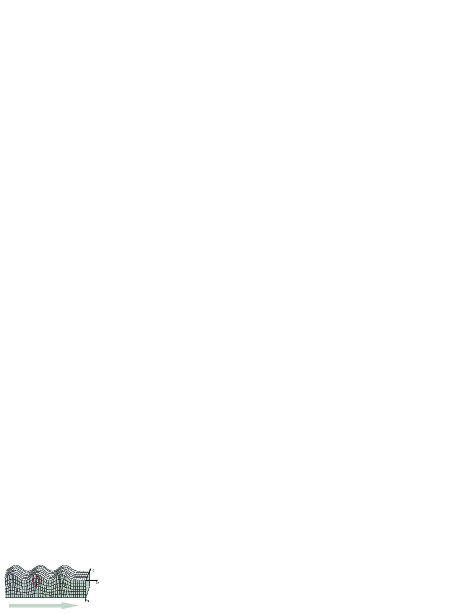
Figure 1: (color online) Geometry of the problem.

Using standard formulas LL for the displacement field in a surface acoustic wave, one obtains

$$\delta{\bm{\phi}}({\bf r})=\frac{1}{2}\frac{\omega}{c_{t}}u_{0}\,e^{-k_{t}y}\cos(kx-\omega t)\,{\bf e}_{z}\equiv\delta\phi(x,t)\,{\bf e}_{z}\,,$$ (3)

where $\omega=c_{t}k\,\xi$, $k_{t}\equiv k\sqrt{1-\xi^{2}}$, $\xi$ is a real number between 0 and 1 satisfying

$$\xi^{6}-8\xi^{4}+8\xi^{3}\left(3-2\frac{c_{t}^{2}}{c_{l}^{2}}\right)-16\left(1-\frac{c_{t}^{2}}{c_{l}^{2}}\right)=0\,,$$ (4)

and $c_{t,l}$ are velocities of transverse and longitudinal sound.

In the presence of deformations of the crystal lattice, local anisotropy axes defined by the crystal field are rotated by the angle given by Eq. (3). In the Hamiltonian, this rotation is equivalent to the rotation of the operator $\hat{\bf S}$ in the opposite direction, which can be performed by the $(2S+1)\times(2S+1)$ matrix in the spin space CGS ,

$$\hat{\bf S}\rightarrow\hat{R}^{-1}\hat{\bf S}\hat{R},\qquad\hat{R}=e^{i\hat{\bf S}\cdot\delta{\bm{\phi}}}\,.$$ (5)

The spin Hamiltonian in the laboratory frame becomes

$$\hat{\mathcal{{H}}}=e^{-i\hat{\bf S}\cdot\delta{\bm{\phi}}}\,\hat{\mathcal{{H}}}_{A}\,e^{i\hat{\bf S}\cdot\delta{\bm{\phi}}}\,.$$ (6)

In order to find the laboratory-frame wave function $|\Psi\rangle$, it is useful to introduce the lattice-frame wave function $|\Psi^{(lat)}\rangle$, defined through the unitary transformation

$$|\Psi^{(lat)}\rangle=e^{i\delta{\bm{\phi}}\cdot\hat{\bf S}}|\Psi\rangle\,.$$ (7)

Differentiating it on time it is easy to see that this function satisfies Schrödinger equation with the lattice-frame Hamiltonian

$$\hat{\mathcal{H}}^{(lat)}=\hat{\mathcal{H}}_{A}-\hbar\hat{\bf S}\cdot{\bf\Omega}$$ (8)

where

$${\bf\Omega}=\frac{\partial\delta{\bm{\phi}}}{\partial t}=\frac{1}{2}\frac{\omega^{2}}{c_{t}}u_{0}\,e^{-k_{t}y}\sin(kx-\omega t)\,{\bf e}_{z}\,.$$ (9)

To this point we have not made any assumptions about the magnitude of $\delta{\bm{\phi}}$, so that the equations (6) and (8) are exact. An interesting observation for the comparison of the effects of ultrasound and ac magnetic field is that the Hamiltonian (8) resembles the Hamiltonian of a particle of spin $\hat{\bf S}$ in the ac magnetic field which amplitude scales as the square of the frequency.

We are interested in the Rabi oscillations between the two lowest states of $\hat{\cal{H}}_{A}$:

$$|\phi_{\pm}\rangle=\frac{1}{\sqrt{2}}(|S\rangle\pm|-S\rangle)\,,$$ (10)

where $|\pm S\rangle$ satisfy $\hat{S}_{z}|\pm S\rangle=\pm S|\pm S\rangle$. It makes sense, therefore, to project our Hamiltonian on the $|\pm S\rangle$ states, making the problem essentially a two-state problem. This gives

$$\hat{h}^{(lat)}_{eff}=-\frac{\Delta}{2}\,\hat{\sigma}_{1}-\hbar\omega_{R}\sin(kx-\omega t)\,\hat{\sigma}_{3}\,,$$ (11)

where $\Delta$ is the energy distance between the ground state $|\phi_{+}\rangle$ and the first excited state $|\phi_{-}\rangle$, $\hat{\sigma}_{1}\equiv|S\rangle\langle-S|+|-S\rangle\langle S|$, $\hat{\sigma}_{3}\equiv|S\rangle\langle S|-|-S\rangle\langle-S|$, and

$$\omega_{R}=\frac{1}{2c_{t}}\,\omega^{2}\,u_{0}\,S\,e^{-k_{t}y}\,.$$ (12)

The two-state approach will be valid if $\Delta$ and $\hbar\omega$ are small in comparison with the distances to other spin levels. Note that the tunnel splitting $\Delta$ originates from the term $\hat{V}$ in $\hat{\cal{H}}_{A}$ that does not commute with $\hat{S}_{z}$.

It is easy to check that at $\omega\sim\Delta/\hbar$, which is our case of interest for consideration of Rabi oscillations, the second term in Eq. (11) can be treated as a perturbation as long as the wavelength of the acoustic wave satisfies $\lambda\gg Su_{0}$. For a not very large $S$ this condition is always fulfilled by surface acoustic waves. The unperturbed eigenstates of the problem are then the eigenstates of $\sigma_{1}$ given by Eq. (10). Their energies are $\pm\Delta/2$. The time-dependent perturbation produces transitions between these states, resulting in the Rabi oscillations when $\hbar\omega\simeq\Delta$. The standard way to obtain the evolution of the wave function is to apply the rotating wave approximation Rabi . Note that the coordinates $x$ and $y$ in Eq. (11) can be viewed as parameters. Expressing the wave function as

$$|\Psi(t)^{(lat)}\rangle=C_{+}(t)|\phi_{+}\rangle+C_{-}(t)|\phi_{-}\rangle\,,$$ (13)

and starting with $C_{-}(0)=0$, $C_{+}(0)=1$ at $t=0,x=0$, one obtains

$$C_{-}(t) = \frac{\omega_{R}}{\Omega_{R}}\,e^{-\frac{i}{2}\,\omega t}\sin\left(\frac{\Omega_{R}t}{2}\right)$$ (14)

$$C_{+}(t) = \left[\cos\left(\frac{\Omega_{R}t}{2}\right)+i\frac{\Delta/\hbar-\omega}{\Omega_{R}}\,\sin\left(\frac{\Omega_{R}t}{2}\right)\right]e^{\frac{i}{2}\,\omega t}\,,$$

where

$$\Omega_{R}=\sqrt{(\Delta/\hbar-\omega)^{2}+\omega_{R}^{2}}\,.$$ (15)

Assuming that every spin was in the ground state $|\phi_{+}\rangle$ before the sound wave arrived, the spatial dependence of the wave function can be obtained by making a replacement $t\rightarrow t-kx/\omega$ in Eq. (14). In the absence of spatial derivatives in the Hamiltonian (11), $|\Psi(t)^{(lat)}\rangle$ is defined up to the phase factor $\exp[i\theta(x,y)]$ with $\theta$ being an arbitrary real function of coordinates. From Eq. (7) the wave function of the system in the laboratory frame is $|\Psi\rangle=e^{-i\delta{\bm{\phi}}\cdot{\bf S}}|\Psi^{(lat)}\rangle$. Because of the smallness of $\delta\phi$, the dynamics of $|\Psi\rangle$ essentially coincides with the dynamics of $|\Psi^{(lat)}\rangle$ and is given by Rabi oscillations between the states $|\phi_{\pm}\rangle$ at the frequency $\Omega_{R}$. This is confirmed by numerical calculations with the lattice-frame and laboratory-frame Hamiltonians, see Fig. 2.

\begin{picture}(20.0,5.4)\centerline{\hbox{\psfig{width=247.53888pt}}} \end{picture}

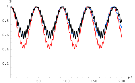
Figure 2: (color online) Time dependence ($t^{\prime}\equiv t\Delta/\hbar$) of the probability to find the spin in the state $|\phi_{+}\rangle$ at $x=0$, $S=10$, $\omega_{R}=0.1\omega$, and $\omega=0.9(\Delta/\hbar)$. Dotted line (red): Numerical result for the laboratory-frame Hamiltonian (19). Dash line (blue): Numerical result for the lattice-frame Hamiltonian (11). Solid line (black): Analytical result given by Eq. (14).

The expectation value of the projection of the spin onto the anisotropy axis (the Z-axis) is given by

$$\langle\Psi(t)|\hat{S}_{z}|\Psi(t)\rangle=2S\frac{\omega_{R}}{\Omega_{R}^{2}}\times$$

$$\bigg{\{}\left(\omega-\frac{\Delta}{\hbar}\right)\sin(\omega t-kx)\sin^{2}\left[\frac{1}{2}\left(\Omega_{R}t-K_{R}x\right)\right]$$

$$+\frac{1}{2}\,\Omega_{R}\cos(\omega t-kx)\sin\left(\Omega_{R}t-K_{R}x\right)\bigg{\}}\,,$$ (16)

where $K_{R}=({\Omega_{R}}/{\omega})k\ll k$ can be called the “Rabi” wave vector. Thus, the space-time Rabi oscillations of the occupation numbers of spin states generate space-time oscillations of the magnetization of the crystal. On resonance, when $\omega=\Delta/\hbar$, Eq. (Rabi oscillations from ultrasound in spin systems) simplifies to

$$\langle\Psi(t)|\hat{S}_{z}|\Psi(t)\rangle=S\cos(kx-\omega t)\sin\left(\omega_{R}t-k_{R}x\right)\,,$$ (17)

with $k_{R}=({\omega_{R}}/{\omega})k\ll k$. The condition $\omega_{R}\ll\omega$ ($Su_{0}\ll\lambda$) implies that the time dependence of $\langle\hat{S}_{z}\rangle$ at any point in space consists of the oscillations at frequency $\omega$ with beats of frequency $\omega_{R}$. Similarly, $\langle\hat{S}_{z}\rangle$ at any moment of time oscillates in space with the wave vector $k$ and exhibits beats with the wave vector $k_{R}\ll k$.

Our conclusions can be checked by obtaining the full solution of the problem in the laboratory frame in a particular case of a biaxial symmetry, when $\hat{V}$ in Eq. (2) equals $E(\hat{S}_{x}^{2}-\hat{S}_{y}^{2})$. In this case Eq. (6) reduces to

$$\hat{\mathcal{H}}=-D\hat{S}_{z}^{2}+\frac{E}{2}\left\{\hat{S}_{+}^{2}e^{-2i\delta\phi(x,t)}+\hat{S}_{-}^{2}e^{2i\delta\phi(x,t)}\right\}\,,$$ (18)

where $\hat{S}_{\pm}=\hat{S}_{x}\pm i\hat{S}_{y}$. The second term can be treated as a perturbation provided that $E\ll D$.

\begin{picture}(20.0,5.4)\centerline{\hbox{\psfig{width=247.53888pt}}} \end{picture}

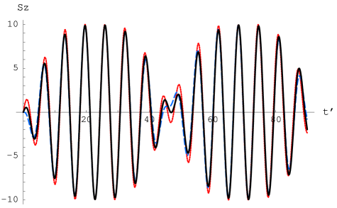
Figure 3: (color online) Time dependence ($t^{\prime}\equiv t\Delta/\hbar$) of the expectation value of the projection of the spin on the anisotropy axis at $x=0$, $S=10$, $\omega_{R}=0.1\omega$ and $\omega=0.9(\Delta/\hbar)$. Dotted line (red): Numerical result for the laboratory-frame Hamiltonian (19). Dash line (blue): Numerical result for the lattice-frame Hamiltonian  (11). Solid line (black): Analytical result given by Eq. (Rabi oscillations from ultrasound in spin systems).

At $\omega\ll(2S+1)D/\hbar\,$ the dynamics of the wave function involves only a superposition of the $|\pm S\rangle$ states. As in the lattice-frame consideration, it is then convenient to project the Hamiltonian (18) onto these two states. In order to obtain such an effective two-state Hamiltonian that accounts for the tunnel splitting of the lowest energy states, one must apply perturbation theory for the degenerate states $|\pm S\rangle$ to the $S$-th order book . This results in

$$\hat{h}_{eff}=-\frac{\Delta}{2}\left\{e^{2iS\delta\phi(x,t)}|S\rangle\langle-S|+e^{-2iS\delta\phi(x,t)}|-S\rangle\langle S|\right\}.$$ (19)

Here $\Delta=8D{(2S)!}{\left[(S-1)!\right]^{-2}}\left({E}/{8D}\right)^{S}$ is the tunnel-splitting for the biaxial model in the absence of lattice distortions Garanin . Numerical solution for $\langle\hat{S}_{z}\rangle$ that follows from Eq. (19), and its comparison with the analytical solution given by Eq. (Rabi oscillations from ultrasound in spin systems), are illustrated in Fig. 3. The beats discussed above are clearly seen in the figure.

We shall now discuss conditions under which the above effects can be observed. The first condition is that the rate of decoherence of the spin states is lower than the frequencies involved. The lowest of these frequencies is $\omega_{R}=2\pi^{2}{f^{2}}u_{0}S/c_{t}$, where $f$, $u_{0}$, and $c_{t}$ are the frequency, the amplitude, and the velocity of the sound. For, e.g., $f=3\,$GHz, $u_{0}=1\,$nm, $S=10$, and $c_{t}=10^{3}$m/s, one obtains $\omega_{R}\sim 2\,$GHz $\ll$ $\omega=2\pi f\sim 20\,$GHz. If such a high value of $\omega_{R}$ were to be produced by an electromagnetic wave, it would require the ac magnetic field of amplitude $10\,$G, which is not easy to achieve in experiment. Note, however, that the Rabi oscillations of $\langle\hat{S}_{z}\rangle$ generated in a crystal of molecular magnets by ultrasound, contrary to the Rabi oscillations generated in a small crystal by an electromagnetic wave, will have a pronounced wave dependence on coordinates so that $\langle\hat{S}_{z}\rangle$ averaged over the wavelength of the sound, $\lambda$, will be zero. Consequently, measurements of the oscillations of $\langle\hat{S}_{z}\rangle$ should be done on the scale that is small compared to $\lambda$.

Another restriction comes from the inevitable presence of the dc magnetic fields that generate the Zeeman energy bias for the $|\pm S\rangle$ states. Such fields can be of dipolar origin or they can be any stray fields in the system. They are not likely to affect our results qualitatively if the Zeeman energy bias is small compared to $\hbar\omega\sim\Delta$. Note that the tunnel splitting, $\Delta$, can be controlled by a transverse magnetic field. Thus, the above condition translates into $B_{l}\leq 2\pi f/(\gamma S)$ for the longitudinal field $B_{l}$. For $f\sim 3\,$GHz one then needs $B_{l}\leq 100\,$G. In the case of a greater bias field (and/or higher decoherence), higher frequencies of the acoustic waves will be required. In principle, surface acoustic waves of frequency as high as $100\,$GHz have been generated in experiment Santos . However, since $\omega_{R}\propto\omega^{2}$, raising $\omega$ significantly may eventually violate the condition $\omega_{R}\ll\omega$ under which our results were derived.

In Conclusion, we have shown that transversal acoustic waves in the GHz range provide spin-rotation coupling that can be used to generate space-time Rabi oscillations in molecular magnets. When frequency of ultrasound, $\omega$, equals the distance between tunnel-split spin states, the magnetization on the surface of the crystal oscillates as $\langle\hat{S}_{z}\rangle=S\cos(kx-\omega t)\sin[\omega_{R}t-k_{R}x]$, where $\omega_{R}={\omega^{2}}u_{0}S/(2c_{t})$ and $k_{R}=(\omega_{R}/\omega)k$, with $u_{0}$ and $c_{t}$ being the amplitude and the speed of the sound respectively.

The authors thank Dmitry Garanin, Javier Tejada, Paulo Santos, and Jaroslav Albert for helpful discussions. This work has been supported by the NSF Grant No. EIA-0310517.

References

- (1) E. M. Chudnovsky and J. Tejada, Lectures on Magnetism (Rinton Press, 2006).
- (2) F.W. Hehl and W.-T. Ni, Phys. Rev. D 42, 2045 (1990).
- (3) S. J. Barnett, Phys. Rev. 6, 239 (1915).
- (4) L. D. Landau and E. M. Lifshitz, Theory of Elasticity (Pergamon, New York, 1959).
- (5) A. Hernández Mínguez, J. M. Hernández, F. Maciá, A. García Santiago, J. Tejada, and P. V. Santos, Phys. Rev. Lett. 95, 217205 (2005).
- (6) A. Hernández Mínguez, F. Maciá, J. M. Hernández, J. Tejada, and P. V. Santos, cond-mat/0609429 (unpublished).
- (7) K. Gottfried and T.-M. Yan, Quantum Mechanics: Fundamentals (Springer-Verlag, 2003).
- (8) L. Sorace, W. Wernsdorfer, C. Thirion, A.-L. Barra, M. Pacchioni, D. Mailly, and B. Barbara, Phys. Rev. B 68, 220407 (2003); K. Petukhov, W. Wernsdorfer, A.-L. Barra, and V. Mosser, Phys. Rev. B 72, 052401 (2005).
- (9) S. Hill, R. S. Edwards, S. I. Jones, N. S. Dalal, and J. M. North, Phys. Rev. Lett. 90, 217204 (2003); S. Hill, R. S. Edwards, N. Aliaga-Alcalde, G. Christou, Science 303, 1015 (2003).
- (10) E. del Barco, A. D. Kent, E. C. Yang, and D. N. Hendrickson, Phys. Rev. Lett. 93, 157202 (2004)
- (11) M. Bal, J. R. Friedman, Y. Suzuki, K. M. Mertes, E. M. Rumberger, D. N. Hendrickson, Y. Myasoedov, H. Shtrikman, N. Avraham, and E. Zeldov Phys. Rev. B 70, 100408 (2004).
- (12) E. M. Chudnovsky, D. A. Garanin, and R. Schilling, Phys. Rev. B 72, 094426 (2005).
- (13) D.A. Garanin, J. Phys. A 24, L61 (1991).
- (14) M. M. de Lima, Jr. and P. V. Santos, Rep. Prog. Phys. 68, 1639 (2005).