Quantum criticality and minimal conductivity in graphene with long-range disorder

Abstract

We consider the conductivity $\sigma_{xx}$ of graphene with negligible intervalley scattering at half filling. We derive the effective field theory, which, for the case of a potential disorder, is a symplectic-class $\sigma$-model including a topological term with $\theta=\pi$. As a consequence, the system is at a quantum critical point with a universal value of the conductivity of the order of $e^{2}/h$. When the effective time reversal symmetry is broken, the symmetry class becomes unitary, and $\sigma_{xx}$ acquires the value characteristic for the quantum Hall transition.

Recent breakthrough in graphene fabrication Novoselov04 and subsequent transport experiments Novoselov05 revealed remarkable electronic properties of this material. One of the most striking experimental observation is the minimal conductivity $\sigma_{xx}$ of order $e^{2}/h$ observed in undoped samples and staying almost constant in a wide range of temperatures $T$ from 300 K down to $\sim 1K$. This behavior should be contrasted to well-established results on the conductivity of two-dimensional (2D) systems where localization effects drive the system into insulating state at low $T$ McCann ; AEA . An apparently $T$-independent value of $\sigma_{xx}\sim e^{2}/h$ suggests that the system is close to a quantum critical point and calls for a theoretical explanation.

One particular class of randomness when this scenario is realized, namely, the chiral disorder, was analyzed in detail in Ref. OurPRB (see also Ref. Ryu ). It was shown that, if one of the chiral symmetries of clean graphene is preserved by disorder, the conductivity at half filling is not affected by localization and is equal to $(4/\pi)e^{2}/h$ (up to small corrections). While various types of randomness in graphene (in particular, dislocations, ripples, or strong point-like defects) do belong to the chiral type, the experimentally observed value of $\sigma_{xx}$ is larger by a factor $\sim 3$, suggesting a different type of criticality. In this paper we consider another broad class of randomness in graphene — long-range disorder. This case has a particular experimental relevance if the conductivity is dominated by charged impurities; the ripples Morpurgo06 ; Meyer07 belong to this class of randomness as well. Numerical simulations of graphene with long-range random potential Nomura06 ; Beenakker_numerics provide an evidence in favor of a scale-invariant conductivity.

The low-energy electron spectrum of clean graphene split into two degenerate valleys. The characteristic feature of the long-range disorder is the absence of valley mixing due to the lack of scattering with large momentum transfer. This allows us to describe the system in terms of a single-valley Dirac Hamiltonian with disorder,

$$H=v_{0}\bm{\sigma}\mathbf{k}+\sigma_{\mu}V_{\mu}(\mathbf{r}).$$ (1)

Here $v_{0}\simeq 10^{8}$ cm/s is the Fermi velocity. The four Pauli matrices $\sigma_{\mu}$ (with $\sigma_{0}=1$) operate in the space of two-component spinors reflecting the sublattice structure of the honeycomb lattice, $\bm{\sigma}=\{\sigma_{1},\sigma_{2}\}$, and disorder includes random scalar ($V_{0}$) and vector ($V_{1,2}$) potentials and random mass ($V_{3}$). The Hamiltonian (1) was considered in Ref. Ludwig as a model for quantum Hall transition.

To derive the field theory, we introduce a vector superfield $\psi$ with $2\times 2\times 2=8$ components: the matrix structure of $H$ in the sublattice space is complemented by the boson–fermion (BF) and the retarded-advanced (RA) structures. Assuming for simplicity Gaussian $\delta$-correlated disorder distribution, we get the action

$$S[\psi]=\int d^{2}r\biggl{[}-i\bar{\psi}\bigl{(}\hat{\varepsilon}+iv_{0}\bm{\sigma}\nabla\bigr{)}\psi+\frac{1}{2}\langle V_{\mu}^{2}\rangle(\bar{\psi}\sigma_{\mu}\psi)^{2}\biggr{]},$$ (2)

with $\hat{\varepsilon}=\varepsilon+i0\Lambda$ where $\Lambda=\mathop{\mathrm{diag}}\{1,-1\}_{RA}$. Assuming the isotropy, the disorder is described by three couplings $\alpha_{0}=\langle V_{0}^{2}\rangle/2\pi v_{0}^{2}$, $\alpha_{\perp}=\langle V_{1}^{2}+V_{2}^{2}\rangle/2\pi v_{0}^{2}$, and $\alpha_{z}=\langle V_{3}^{2}\rangle/2\pi v_{0}^{2}$. On short (ballistic) scales the parameters of (2) are renormalized Ludwig ; Nersesyan ; AEA ; OurPRB ; the effective theory on longer scales is the non-linear sigma model Efetov .

The clean single-valley Hamiltonian (1) obeys the effective time-reversal (TR) invariance $H=\sigma_{2}H^{*}\sigma_{2}$. This symmetry (denoted as $T_{\perp}$ in Ref. OurPRB ) is not the physical TR symmetry: the latter interchanges the nodes and is of no significance in the absence of inter-node scattering. If the only disorder is random scalar potential, the TR invariance is not broken and the system falls into the symplectic symmetry class (AII) Ludwig ; McCann ; AEA . The standard realization of such symmetry is a system with spin-orbit coupling; in the present context the role of spin is played by the sublattice space.

We start with a more generic case of the unitary symmetry (class A). The TR invariance is broken as soon as a (either random or non-random) mass or vector potential is included, in addition to the scalar potential. We find it instructive to present the derivation for a system with a non-zero mass term $m\sigma_{3}$. Decoupling the $\psi^{4}$ term by a supermatrix field $Q$ and integrating out $\psi$, we get

$$S[Q]=\mathop{\mathrm{Str}}\left[-\frac{\gamma^{2}Q^{2}}{4\pi v_{0}^{2}\alpha_{0}}+\ln\Bigl{(}\varepsilon-m\sigma_{3}+iv_{0}\bm{\sigma}\nabla+i\gamma Q\Bigr{)}\right],$$ (3)

where Str includes the matrix supertrace and the spatial integration, $\gamma=1/2\tau$, and $\tau$ is the mean free time.

The saddle-point approximation footnote_critical reduces the set of $Q$ to the conventional manifold of the unitary $\sigma$-model; the relevant $Q$’s are $4\times 4$ supermatrices operating in RA and BF spaces and satisfying the constraint $Q^{2}=1$. The low-energy modes describe slow spatial variation of $Q$ on this manifold, and the effective theory is the result of the gradient expansion of the action (3) in these modes. As we show, this expansion is highly non-trivial due to anomalies in the theory of Dirac fermions Haldane , which induce a topological contribution to the $\sigma$-model Bocquet .

We first perform the gradient expansion of the real part of the action (3)

$$S_{1}[Q]=(1/2)\mathop{\mathrm{Str}}\ln\Bigl{(}G_{+}^{-1}G_{-}^{-1}+v_{0}\gamma\bm{\sigma}\nabla Q\Bigr{)}.$$ (4)

Here the matrix Green functions defined as $G_{\pm}^{-1}=\varepsilon-m\sigma_{3}+i\bm{\sigma}\nabla\pm i\gamma\Lambda$ are diagonal in RA space with retarded and advanced Green functions as their elements, $G_{+}=\mathop{\mathrm{diag}}\{G^{R},G^{A}\}$, $G_{-}=\mathop{\mathrm{diag}}\{G^{A},G^{R}\}$. Expanding Eq. (4) to the second order in $\nabla Q$ and using the identity $G^{R}-G^{A}=-2i\gamma G^{R}G^{A}$, we get the familiar gradient term,

$$S_{1}[Q]=(\sigma_{xx}/8)\mathop{\mathrm{Str}}\bigl{(}\nabla Q\bigr{)}^{2}.$$ (5)

The factor $\sigma_{xx}$ in Eq. (4) is identified as the dimensionless (in units $e^{2}/h$) longitudinal conductivity given by

$$\sigma_{xx}=-(v_{0}^{2}/2)\mathop{\mathrm{Tr}}\Bigl{[}\bigl{(}G^{R}-G^{A}\bigr{)}\sigma_{x}\bigl{(}G^{R}-G^{A}\bigr{)}\sigma_{x}\Bigr{]}\\ =(1/2\pi)\left[1+f(\varepsilon,m)(\varepsilon^{2}+\gamma^{2}-m^{2})/2\gamma\right],$$ (6)

where we introduced the notation

$$f(x,y)=x^{-1}\{\arctan[(x+y)/\gamma]+\arctan[(x-y)/\gamma]\}.$$

The calculation of the imaginary part $iS_{2}[Q]$ is much more subtle. We use the representation $Q=T^{-1}\Lambda T$ and cycle the matrices under the supertrace. The resulting expression depends on the vector $\mathbf{u}=T\nabla T^{-1}$,

$$iS_{2}[Q]=(1/2)\mathop{\mathrm{Str}}\Bigl{[}\ln\bigl{(}G_{+}^{-1}+iv_{0}\bm{\sigma}\mathbf{u}\bigr{)}-\ln\bigl{(}G_{-}^{-1}+iv_{0}\bm{\sigma}\mathbf{u}\bigr{)}\Bigr{]}.$$

The permutation of matrices leading to this formula is equivalent to a rotation of fermion fields, $\psi\mapsto T\psi$, in Eq. (2). This is not an innocent procedure in view of quantum anomaly Fujikawa80 . However, such anomalous contributions from the two logarithms cancel in $iS_{2}[Q]$. We proceed with expanding $iS_{2}[Q]$ in powers of $\mathbf{u}$. The first two terms of this expansion are

$$iS_{2}^{(1)}\!=(iv_{0}/2)\mathop{\mathrm{Str}}\bigl{[}\Lambda\bigl{(}G^{R}-G^{A}\bigr{)}\bm{\sigma}\mathbf{u}\bigr{]}\equiv\pi\mathop{\mathrm{Str}}\bigl{(}\Lambda\mathbf{J}\mathbf{u}\bigr{)},$$ (7)

$$\!iS_{2}^{(2)}\!=\frac{\sigma_{xy}^{I}\epsilon_{\alpha\beta}}{2}\mathop{\mathrm{Str}}\bigl{(}u_{\alpha}\Lambda u_{\beta}\bigr{)}\!=\frac{\sigma_{xy}^{I}}{4}\mathop{\mathrm{Str}}\bigl{(}Q\nabla_{x}Q\nabla_{y}Q\bigr{)}.$$ (8)

The factors in Eqs. (7), (8) are the current spectral density $\mathbf{J}(\mathbf{r})$ and the classical part of Hall conductivity Pruisken

$$\sigma_{xy}^{I}=(v_{0}^{2}/2)\mathop{\mathrm{Tr}}\Bigl{[}\bigl{(}G^{R}+G^{A}\bigr{)}\sigma_{x}\bigl{(}G^{R}-G^{A}\bigr{)}\sigma_{y}\Bigr{]}\\ =-(m/2\pi)\;f(\varepsilon,m).$$ (9)

The net current, and hence the linear term (7), is absent in the bulk of the system. It is incorrect, however, to drop this term. The contribution $iS_{2}^{(1)}$ accounts for the edge current and gives the quantum part of the Hall conductivity Pruisken . Prior to considering it, we have to establish boundary conditions (BC) for the Hamiltonian (1).

Generically, BC in realistic graphene mix states from the two valleys of the spectrum. We can stay, however, within the single-valley model and assume an infinite mass $M\to\infty$ at the boundary of the sample BerryMondragon . Localization effects described by the $\sigma$-model occur in the bulk and hence are insensitive to particular BC. We thus assume that $m(\mathbf{r})$ changes from a constant value $m$ inside the sample to another, large value $M$ outside it. The gradient of mass is not zero near the edge only. We further assume that the mass variation is slow on the scale of the electron mean free path but fast compared to $\sigma$-model length scales. This allows us to perform an expansion of the Green functions in Eq. (7) in $\nabla m$. With the help of identity $[\mathbf{r},G]=iv_{0}G\bm{\sigma}G$, we obtain

$$J_{\alpha}(\mathbf{r})=-(v_{0}^{2}/2\pi)\;\nabla_{\beta}m\;\mathop{\mathrm{tr}}\Bigl{[}\sigma_{\alpha}G^{R}\sigma_{3}G^{R}\sigma_{\beta}G^{R}\\ -\sigma_{\alpha}G^{A}\sigma_{3}G^{A}\sigma_{\beta}G^{A}\Bigr{]}_{\mathbf{r},\mathbf{r}}=\frac{\epsilon_{\alpha\beta}}{2\pi}\;\frac{\partial\sigma_{xy}^{II}}{\partial m}\;\nabla_{\beta}m.$$ (10)

The emerged trace is a mass derivative of the quantum part $\sigma_{xy}^{II}$ of Hall conductivity Pruisken ; its direct calculation and subsequent integration with respect to $m$ yields

$$\sigma_{xy}^{II}=-(m/2\pi)\;f(m,\varepsilon).$$ (11)

Substituting (10) in (7) and integrating over the boundary strip, we express the term (7) as an integral along the edge and then apply the Stokes theorem:

$$iS_{2}^{(1)}=\frac{\epsilon_{\alpha\beta}}{2}\Bigl{[}\sigma_{xy}^{II}(m)-\sigma_{xy}^{II}(M)\Bigr{]}\mathop{\mathrm{Str}}\bigl{(}\Lambda\nabla_{\alpha}u_{\beta}\bigr{)}\\ =\frac{1}{4}\biggl{(}\sigma_{xy}^{II}+\frac{\mathop{\mathrm{sgn}}M}{2}\biggr{)}\mathop{\mathrm{Str}}\bigl{(}Q\nabla_{x}Q\nabla_{y}Q\bigr{)}.$$ (12)

To derive the last expression, we have used the identity $\epsilon_{\alpha\beta}\nabla_{\alpha}u_{\beta}=\epsilon_{\alpha\beta}u_{\beta}u_{\alpha}$ and the value of $\sigma_{xy}^{II}$ in the limit of infinitely large $M$. The same result is obtained if one uses alternative BC introducing the second node with the large mass $M$. In that case, $(1/2)\mathop{\mathrm{sgn}}M$ will enter the action as the contribution of the second node to $\sigma_{xy}$ (cf. Refs. Ludwig ; Haldane ). Both contributions to $iS_{2}[Q]$, Eqs. (8) and (12), contain the functional $\mathop{\mathrm{Str}}(Q\nabla_{x}Q\nabla_{y}Q)\equiv 16i\pi N[Q]$ that is a well-known topological invariant on the $\sigma$-model manifold Pruisken ; its possible values are integer multiples of $16\pi i$. The imaginary part of the action is defined up to a multiple of $2\pi i$. Thus the sign of $M$ is irrelevant, as expected: the bulk theory should not be sensitive to BC.

Collecting all the contributions, we get the $\sigma$-model action for the single-node Dirac fermions with mass $m$:

$$S[Q]=\frac{1}{4}\mathop{\mathrm{Str}}\left[-\frac{\sigma_{xx}}{2}(\nabla Q)^{2}+\biggl{(}\sigma_{xy}+\frac{1}{2}\biggr{)}Q\nabla_{x}Q\nabla_{y}Q\right].$$ (13)

The topological term is equal to $i\theta N[Q]$, with the angle $\theta=2\pi\sigma_{xy}+\pi$. In graphene the mass $m$ is absent, so that $\sigma_{xy}=0$. Thus, the topological angle is $\theta=\pi$. The theory (13) is then exactly on the critical line of the quantum Hall transition Pruisken , in agreement with the arguments of Ref. Ludwig . Thus the graphene with a generic (TR breaking) long-range disorder is driven into the quantum Hall critical point, with the conductivity $4\sigma^{*}_{U}$ (the factor 4 accounts for the spin and valley degeneracy). The value $\sigma^{*}_{U}$ is known to be in the range $\sigma^{*}_{U}\simeq 0.5-0.6$ from numerical simulations Quantum-Hall_critical . A schematic scaling function in this case is shown in Fig. 1a. While formally this result holds for any energy $\varepsilon$, in reality it only works near half filling (where the bare conductivity is $\sim e^{2}/h$); for other $\varepsilon$ the quantum Hall critical point would only be reached for unrealistic temperatures and system sizes.

Let us now turn to the case of preserved TR invariance, describing in particular charged impurities. The system belongs then to the symplectic symmetry class AII. The derivation of the $\sigma$-model starts with the doubling of $\psi$ variables accounting for the TR symmetry Efetov . Then $Q$ is $8\times 8$ matrix obeying an additional constraint of charge conjugation $Q=\bar{Q}$. The real part of the action is calculated in the same way as in the unitary case, yielding Eq. (4) with an additional factor $1/2$.

Since the partition function of the symplectic model is real, the imaginary part of the action $S_{2}[Q]$ can take one of the two possible values, $0$ or $\pi$. The discreteness of $S_{2}[Q]$ suggests that it again should be proportional to a topological invariant on the $\sigma$-model manifold. A non-trivial topology may arise only in the compact (fermion) sector of $Q$. The corresponding target space is $\mathcal{M}_{F}=O(4n)/O(2n)\times O(2n)$, where $n$ is the number of fermion species. While for the conventional (“minimal”) $\sigma$-model $n=1$, larger values will arise if one considers higher-order products of Green functions. The topological invariant takes values from the homotopy group ViroFuchs

$$\pi_{2}\bigl{[}\left.\mathcal{M}_{F}\right|_{n=1}\bigr{]}=\mathbb{Z}\times\mathbb{Z},\qquad\pi_{2}\bigl{[}\left.\mathcal{M}_{F}\right|_{n\geq 2}\bigr{]}=\mathbb{Z}_{2}.$$ (14)

The homotopy group in the case $n=1$ is richer than for $n\geq 2$. Nevertheless, $S_{2}[Q]$ may take only two non-equivalent values. Hence only a certain $\mathbb{Z}_{2}$ subgroup Fendley of the whole $\mathbb{Z}\times\mathbb{Z}$ comes into play as expected: the phase diagram of the theory should not depend on $n$.

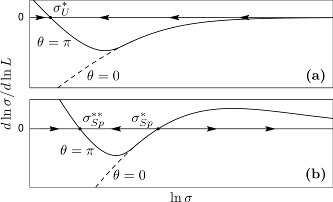
Figure 1: Schematic scaling functions for (a) unitary and (b) symplectic universality class with topological term $\theta=\pi$. The ordinary case $\theta=0$ is shown by dashed lines.

To demonstrate the emerging topology explicitly and to calculate the topological invariant, let us analyze the case $n=1$ in more detail. The generators of the compact sector are Hermitian skew-symmetric $4\times 4$ matrices anticommuting with $\Lambda\equiv\rho_{3}$: $\rho_{1}\tau_{2}$, $\rho_{2}\tau_{0}$, $\rho_{2}\tau_{1}$, and $\rho_{2}\tau_{3}$. Here $\rho_{i}$ and $\tau_{i}$ are Pauli matrices in RA and TR space respectively. These generators split into two mutually commuting pairs, each generating a 2-sphere (“diffuson” and “Cooperon” sphere). Simultaneous inversion of both spheres leaves $Q$ intact. Hence the compact sector of the model is the manifold $(S_{2}\times S_{2})/\mathbb{Z}_{2}$. Thus two topological invariants, $N_{1,2}[Q]$, counting the covering of each sphere, emerge in accordance with Eq. (14). The most general topological term is $iS_{2}=i\theta_{1}N_{1}+i\theta_{2}N_{2}$. Due to the TR symmetry, the action is invariant under interchanging the diffuson and Cooperon spheres, which yields $\theta_{1}=\theta_{2}\equiv\theta$ where $\theta$ is either $0$ or $\pi$. The explicit expression for $n=1$ topological term can be written using $\mathbf{u}=T\nabla T^{-1}$

$$iS_{2}[Q]=\frac{\epsilon_{\alpha\beta}}{8}\mathop{\mathrm{Str}}\bigl{[}(\Lambda\pm 1)\tau_{2}u_{\alpha}u_{\beta}\bigr{]}\equiv i\pi(N_{1}[Q]+N_{2}[Q]),$$

yielding $\theta=\pi$. The sign ambiguity here does not affect any observables. If the TR symmetry is broken, the Cooperon modes are frozen and the manifold is reduced to a single diffuson sphere with $iS_{2}[Q]=i\pi N_{1}[Q]$.

The ordinary symplectic theory with no topological term exhibits a metal-insulator transition at $\sigma^{*}_{Sp}\approx 1.4$ Schweitzer . If the conductivity is smaller than this critical value the localization drives the system into insulating state, while in the metallic phase, $\sigma>\sigma^{*}_{Sp}$, antilocalization occurs. Using the analogy with the quantum Hall transition in the unitary class, we argue that the topological term with $\theta=\pi$ suppresses localization effects when the conductivity is small, leading to appearance of a new attracting fixed point at $\sigma^{**}_{Sp}$. The position of the metal-insulator transition, $\sigma^{*}_{Sp}$, is also affected by the topological term. However, we believe that its change is negligible: the instanton correction to the scaling function at large conductivity is exponentially small Pruisken , and the value of the exponential factor $e^{-4\pi\sigma}$ is still extremely small at $\sigma=\sigma^{*}_{Sp}$. A plausible scaling of the conductivity in the symplectic case with $\theta=\pi$ is sketched in Fig. 1. The existence and position of the new critical point can be verified numerically. Recent simulations of graphene Nomura06 ; Beenakker_numerics indeed demonstrate the stability of the conductivity in the presence of long-range disorder. Of course, in reality there will be always a weak inter-valley scattering, which will establish the localization and lowest $T$, in agreement with AEA . However, the approximate quantum criticality will hold in a parametrically broad range of $T$.

Finally, we discuss a connection between our findings and recent results on the quantum spin Hall (QSH) effect in systems of Dirac fermions with spin-orbit coupling KaneMele , which in the presence of random potential also belong to the symplectic symmetry class. Such systems were found to possess two distinct insulating phases, both having a gap in the bulk electron spectrum but differing by the edge properties. While the normal insulating phase has no edge states, the spin-Hall insulator is characterized by a pair of mutually time-reversed spin-polarized edge states penetrating the bulk gap. The transition between these two phases is driven by Rashba spin-orbit coupling strength. The existence of the edge states was attributed to certain $\mathbb{Z}_{2}$ topological index different from one studied above. This topological order is robust with respect to disorder, even if the latter mixes the valleys. The 2D $\sigma$-model is insensitive to the edge properties of the sample and does not capture the difference between the two insulating phases. A suitable effective theory is the one-dimensional (1D) $\sigma$-model for the edge states. The corresponding topological index characterizes the homotopy group $\pi_{1}(\mathcal{M}_{F})$. This group is again $\mathbb{Z}_{2}$ that enables a $\theta$-term with $\theta$ equal to $0$ or $\pi$. The topological term with $\theta=\pi$ is present if the number of channels is odd. Then the conductivity of the 1D system equals $e^{2}/h$ in the long-length limit Takane : one conducting channel survives localization. This is what happens in QSH systems when a pair of edge states is not localized KaneMele . In the presence of disorder, such systems will possess three phases: metal, normal insulator, and QSH insulator. We expect that generically there will be a transition between the latter two. The critical theory discussed in the present work (2D symplectic $\sigma$-model with $\theta=\pi$) should then describe this QSH transition.

In summary, graphene with long-range disorder shows quantum criticality at half filling. If the effective TR symmetry of the single-valley system is preserved (e.g. when Coulomb scatterers are the dominant disorder), the relevant theory is the symplectic $\sigma$-model with topological angle $\theta=\pi$ and the minimal conductivity takes a universal value $4\sigma^{**}_{Sp}$. If the TR symmetry is broken (e.g. by effective random magnetic field due to ripples), the system falls into the universality class of the quantum Hall critical point, with another universal value $\sigma_{xx}=4\sigma^{*}_{U}$. We have argued that the symplectic critical point describes also the QSH transition KaneMele .

We thank F. Evers, Y. Makhlin, V. Serganova, and I. Zakharevich for valuable discussions. The work was supported by the DFG – Center for Functional Nanostructures and by the EUROHORCS/ESF (IVG).

References

- (1) K.S. Novoselov et al., Science 306, 666 (2004).
- (2) K.S. Novoselov et al., Nature 438, 197 (2005); Nature Physics, 2, 177 (2006); Y. Zhang et al., Nature 438, 201 (2005); Phys. Rev. Lett. 96, 136806 (2006); S.V. Morozov et al., ibid 97, 016801 (2006).
- (3) E. McCann et al., Phys. Rev. Lett. 97, 146805 (2006);
- (4) I.L. Aleiner and K.B. Efetov, Phys. Rev. Lett. 97, 236801 (2006); A. Altland, ibid 97, 236802 (2006).
- (5) P.M. Ostrovsky, I.V. Gornyi, and A.D. Mirlin, Phys. Rev B 74, 235443 (2006).
- (6) S. Ryu et al, cond-mat/0610598.
- (7) A.F. Morpurgo and F. Guinea, Phys. Rev. Lett. 97, 196804 (2006).
- (8) J.C. Meyer et al., cond-mat/0701379.
- (9) K. Nomura and A.H. MacDonald, cond-mat/0606589.
- (10) A. Rycerz, J. Tworzydlo, and C.W.J. Beenakker, cond-mat/0612446.
- (11) A.W.W. Ludwig et al., Phys. Rev. B 50, 7526 (1994).
- (12) A.A. Nersesyan, A.M. Tsvelik, and F. Wenger, Nucl. Phys. B 438, 561 (1995).
- (13) K. B. Efetov, Supersymmetry in disorder and chaos (Cambridge University Press, Cambridge, 1996).
- (14) Strictly speaking, saddle-point approximation requires , whereas at . This should not, however, affect the universal critical behavior of the theory governed by symmetry and topology of the problem.
- (15) F.D.M. Haldane, Phys. Rev. Lett. 61, 2015 (1988).
- (16) An alternative route from the Dirac anomaly to a topological term employs non-abelian bosonization, see M. Bocquet, D. Serban, and M.R. Zirnbauer, Nucl. Phys. B 578, 628 (2000); A. Altland, B.D. Simons, and M.R. Zirnbauer, Phys. Rep. 359, 283 (2002).
- (17) K. Fujikawa, Phys. Rev. D 21, 2848 (1980).
- (18) A.M.M. Pruisken, Nucl. Phys. B 235, 277 (1984); in The Quantum Hall Effect ed. by R.E. Prange and S.M. Girvin (Springer, 1987), p. 117.
- (19) M.V. Berry and R.J. Mondragon, Proc. R. Soc. Lond. A 412, 53 (1987).
- (20) Y. Huo, R.E. Hetzel, and R.N. Bhatt, Phys. Rev. Lett. 70, (1993); B.M. Gammel and W. Brenig, ibid 73, 3286 (1994); Z. Wang, B. Jovanović, and D.-H. Lee, ibid 77, 4426 (1996); S. Cho and M.P.A. Fisher, Phys. Rev. B 55 (1997); L. Schweitzer and P. Markoš, Phys. Rev. Lett. 95, 256805 (2005).
- (21) D.B. Fuchs and O.Ya. Viro, Topology II, in series Encyclopaedia of Mathematical Sciences ed. by V.A. Rokhlin and S.P. Novikov, Vol. 24 (Springer, 2004).
- (22) Possibility of the topological term in the 2D symplectic sigma model was emphasized in P. Fendley, Phys. Rev. B 63, 104429 (2001).
- (23) P. Markoš and L. Schweitzer, J. Phys. A 39, 3221 (2006).
- (24) C.L. Kane and E.J. Mele, Phys. Rev. Lett. 95, 146802 and 226801 (2005); L. Sheng et al., ibid 95, 136602 (2005); B.A. Bernevig, T.L. Hughes, and S.-C. Zhang, Science 314, 1757 (2006); M. Onoda, Y. Avishai, and N. Nagaosa, cond-mat/0605510
- (25) T. Ando and H. Suzuura, J. Phys. Soc. Jpn. 71, 2753 (2002); Y. Takane, ibid, 73, 1430 (2004); H. Sakai and Y. Takane, ibid 75, 054711 (2006). Delocalization in 1D symplectic class appeared earlier in M.R. Zirnbauer, Phys. Rev. Lett. 69, 1584-1587 (1992); A.D. Mirlin, A. Müller-Groeling, and M.R. Zirnbauer, Ann. Phys. 236, 325 (1994), but the distinction between even and odd number of channels was not understood there.