Statistics of random voltage fluctuations and the low-density residual conductivity of graphene

Abstract

We consider a graphene sheet in the vicinity of a substrate, which contains charged impurities. A general analytic theory to describe the statistical properties of voltage fluctuations due to the long-range disorder is developed. In particular, we derive a general expression for the probability distribution function of voltage fluctuations, which is shown to be non-Gaussian. The voltage fluctuations lead to the appearance of randomly distributed density inhomogeneities in the graphene plane. We argue that these disorder-induced density fluctuations produce a finite conductivity even at a zero gate voltage in accordance with recent experimental observations. We determine the width of the minimal conductivity plateau and the typical size of the electron and hole puddles. We also propose a simple self-consistent approach to estimate the residual density and the non-universal minimal conductivity in the low-density regime. The existence of inhomogeneous random puddles of electrons and holes should be a generic feature of all graphene layers at low gate voltages due to the invariable presence of charged impurities in the substrate.

I Introduction

Charge inhomogeneities are known to play an important role in understanding transport properties of semiconductors. The randomly positioned impurity ions give rise to a random electrostatic potential and to local modulations of the electron density. The corresponding phenomena have been extensively studied in bulk three-dimensional semiconductors and two-dimensional semiconductor heterostructures. Efros et al. (1993) Recently, it became clear that in graphene, Novoselov et al. (2004) which is a zero-gap semiconductor, the effects of Coulomb disorder on transport are even more drastic.

A particularly interesting property of graphene transport, dubbed the “minimal conductivity,” is a saturation of the conductivity, which happens at a low gate voltage with a width of $\Delta V_{g}\sim 0.5~{}eV$, which is strongly sample dependent. The minimal conductivity value itself is controversial with both a universal conductivity Novoselov et al. (2005) and a sample-dependent non-universal minimal conductivity Zhang et al. (2005) being claimed in the experimental literature. Perhaps the most remarkable feature of this low-density residual conductivity is the approximate saturation of the minimum conductivity with a voltage width of $\Delta V_{g}$, without it dropping to zero at $V_{g}=0$, as the density is lowered from an approximately linear voltage dependence of the conductivity at high density kn:hwang2006c ; Nomura and MacDonald (2006). Although there are transport theories of Dirac fermions in a “white-noise” disordered potential Fradkin (1986) or in clean systems Katsnelson (2006), which give a universal conductivity at the Dirac point, both the measured value of the (non-universal) minimal conductivity and the observed existence of a saturation region around $V_{g}=0$ are in direct conflict with the intrinsic Dirac point physics.

Recent experiments Tan et al. (2007) have convincingly proven that the observed phenomenon of “minimal conductivity” occurs due to charge disorder trapped in the SiO₂ substrate. Each charged ion produces a potential in the graphene layer, which locally mimics a gate voltage and thus leads to a non-zero density in the corresponding region even if the applied gate voltage is zero (i.e., at the “Dirac point”). If the substrate is electrically neutral, the charges in the substrate do produce local density inhomogeneities of electrons and holes, but the total density is zero. The physical picture is that of potential valleys that define electron puddles and mountains that define conducting hole puddles kn:hwang2006c . For the case of charge neutrality, the point of zero external gate voltage defines the percolation threshold, in the sense that the areas where the hole and electron densities are non-zero are exactly equal to one half of the total area of the sample (which is the percolation threshold in two dimensions by duality). By changing the external gate voltage, one creates an excess of electrons or holes and only one type of carrier percolates. As long as the external gate voltage is much smaller than the typical voltage fluctuation due to charged impurities, $V_{\rm g}\ll\sqrt{\overline{V^{2}}}$, the conductivity is mostly determined by the random voltage fluctuations and is almost independent of $V_{\rm g}$. In this case, the conductivity dependence is expected to have a plateau of width $\sqrt{\overline{V^{2}}}$ and be symmetric with respect to $V_{\rm g}\to-V_{\rm g}$. The second scenario that should be considered is a substrate, which is not electro-neutral (which is perhaps a more experimentally relevant picture). In this case, the dependence of the conductivity on the gate voltage is not symmetric with respect to $V_{\rm g}\to-V_{\rm g}$, but is shifted left or right, depending on the substrate’s total charge. The percolation picture still holds, and in two dimensions, the duality between the percolating cluster and its shoreline guarantees that the critical gate voltage at which the electrons stop percolating is the same as that at which the holes begin to percolate. The transition happens at some point $V_{\rm g}\sim\overline{V}$. The width of the minimal conductivity plateau is expected to be of order $\sqrt{\overline{\delta V^{2}}}$. At gate voltages much larger than this value, transport is expected to be insensitive to the voltage fluctuations and is described in terms of the standard transport theory developed earlier by two of the authors kn:hwang2006c . We should mention that the picture outlined above is entirely classical. At the lowest temperatures, the localization physics should become important. However, we believe that the current experiments are being done in the temperature regime where the quantum interference corrections are irrelevant - a quantitative agreement between the available experimental data at high carrier density and the Boltzmann theory of Ref. [kn:hwang2006c, ] strongly support this claim.

To describe the inhomogeneous density profile and transport near the Dirac point in graphene, it is important to have a complete description of the statistical properties of the corresponding random electrostatic potential, which creates the inhomogeneous structure in the first place. In this paper, we develop a systematic analytic theory to derive the relevant probability distribution functions of voltage fluctuations and correlators of voltages due to the charge inhomogeneities. We note here that similar potential fluctuations due to randomly distributed charges have been considered previously in the literature in the context of electron transport in semiconductor heterostructures. E.g., Refs. [Efros et al., 1993,Nixon, ] have studied the statistics of potential and density fluctuations numerically in the framework of a non-linear screening model. Below, we study the voltage fluctuations analytically. Using the developed method, we show that the PDF of voltage fluctuations is generally non-Gaussian and derive explicit analytic expressions for the PDF in various limits. Using the obtained analytical results, we estimate the typical size of charge-disorder-induced electron/hole puddles for a typical graphene sheet. The corresponding results appear to be in a very good agreement with the available experimental data. GG We also suggest a self-consistent (mean-field-like) procedure to estimate the typical density at the Dirac point and the remanent conductivity near the percolation threshold. We also discuss the relation between the suggested percolation-like picture of graphene transport near the Dirac point and the usual diagrammatic transport theory, which works well at high gate voltages.

II General method of calculating statistics of voltage fluctuations

Let us consider a two-dimensional plane in the vicinity of a substrate containing randomly positioned charged impurities. Carriers in the 2D plane screen the bare Coulomb potential produced by the charges in the substrate. The screening properties and the corresponding effective potential depend on the nature and the density of the carriers, but for the purpose of this section, the exact form of the potential is not important. Let us denote it as $v({\bf r})$.

To derive the PDF of voltage fluctuations, we exploit a method, used e.g. by Larkin et al. Larkin et al. (1971) in the context of a mean-field approach to random spin systems. First, we define the PDF as follows

$$P[V]=\left\langle\delta\left[V-\sum_{i}v({\bm{\rho}}_{i})\right]\right\rangle,$$ (1)

where $V$ is the random voltage, the index $i$ in the sum labels the charges, $v({\bm{\rho}}_{i})$ is the potential produced by the $i$-th impurity, and the angular brackets correspond to averaging over all possible positions of impurities. Using the standard representation of the $\delta$-function, we get

$$P[V]=\int\frac{d\lambda}{2\pi}e^{iV\lambda}\left\langle\prod_{i}\exp\left[-i\lambda v({\bm{\rho}})\right]\right\rangle.$$ (2)

At this point, we assume that the impurities are uncorrelated, which allows us to exchange the averaging operation with the product over the impurities in Eq. (2). We obtain

$$P[V]=\int\frac{d\lambda}{2\pi}e^{iV\lambda}\left\langle\exp\left[-i\lambda v({\bm{\rho}})\right]\right\rangle^{N_{\rm imp}},$$ (3)

where $N_{\rm imp}$ is the number of impurities in the substrate. Now, we average over all possible positions of impurities, which have the equal probabilities. This implies simply evaluating an integral over the entire two-dimensional area ${\cal A}$.

$$\left\langle\exp\left[-i\lambda v({\bm{\rho}})\right]\right\rangle=1-\frac{1}{\cal A}\int\limits_{\cal A}d^{2}\rho\left\{1-\exp\left[-i\lambda v({\bm{\rho}})\right]\right\},$$ (4)

where we performed a trivial operation of subtracting and adding a unity. Using Eq. (4), we see that in thermodynamic limit, the PDF can be written as

$$P[V]=\int\frac{d\lambda}{2\pi}e^{iV\lambda}\exp\left[n_{\rm imp}\int\limits d^{2}\rho\left\{1-\exp\left[i\lambda v({\bm{\rho}})\right]\right\}\right],$$ (5)

where $n_{\rm imp}=N_{\rm imp}/{\cal A}$ is the concentration of impurities. Note that this result does not depend on the specific form of the potential and is completely general. We emphasize here that Eq. (5) describes a random potential due to a charged substrate, which contains disorder of just one type. If the substrate contains charges of different types, at the level of Eq. (4), we have to perform another averaging over the distribution function of charges, $C[Q]$. In particular, if the substrate is electroneutral and contains charges of two types of opposite signs $\pm Q_{0}$, then the charge distribution function is simply $C[Q]=\frac{1}{2}\left[\delta(Q-Q_{0})+\delta(Q+Q_{0})\right]$, which leads to the following PDF for the electrically neutral substrate:

$$P_{0}[V]=\int\frac{d\lambda}{2\pi}e^{iV\lambda}\exp\left[n_{\rm imp}\int\limits d^{2}\rho\left\{1-\cos\left[\lambda v({\bm{\rho}})\right]\right\}\right].$$ (6)

To describe the distribution and sizes of disorder-induced droplets, we also consider another PDF function, which determines the distribution of voltages in two different points in the film. Similarly to Eq. (1), we define it as

$$P[V_{1},V_{2},\rho_{12}]=\left\langle\delta\left[V_{1}-\sum_{i}v({\bm{\rho}}_{i1})\right]~{}\delta\left[V_{2}-\sum_{j}v({\bm{\rho}}_{j2})\right]\right\rangle,$$ (7)

where ${\bm{\rho}}_{ij}={\bm{\rho}}_{i}-{\bm{\rho}}_{j}$ is the distance between the two points. This correlation function (7) determines the conditional probability of finding a voltage $V_{2}$ in the point ${\bm{\rho}}_{12}$, provided that in the origin, the voltage is equal to $V_{1}$. Thus, the decay of this correlation function will determine the typical size of the charge disorder-induced puddles of electrons or holes.

Following the simple steps, which led to Eq. (5), we obtain for Eq. (7)

$$P[V_{1},V_{2},\rho_{12}]=\int\frac{d\lambda_{1}d\lambda_{2}}{(2\pi)^{2}}e^{iV_{1}\lambda_{1}-i\lambda_{2}V_{2}}$$ (8)

$$\times\exp\left[n_{\rm imp}\int\limits d^{2}\rho_{0}\left\{1-\exp\left[i\lambda_{2}v({\bm{\rho}}_{20})-i\lambda_{1}v({\bm{\rho}}_{01})\right]\right\}\right].$$

Formally, Eqs. (5) and (8) completely describe the probability distribution of voltages for a given effective interaction, $v({\bf r})$. However, exact analytical calculation of the full PDFs is possible only in the simplest cases of pure Coulomb interaction and large-distance asymptote of the linearly screened Coulomb (see below Sec. III). To correctly interpolate between the two behaviors, one has to consider the general form of the screened interaction potential. The latter has a relatively complicated structure in real space and generally it is not possible to calculate the full PDF analytically. However, it is possible to evaluate exactly the relevant moments of the PDF. These moments can be calculated from Eqs. (5) and (8), by simply evaluating derivatives with respect to the auxiliary parameter $\lambda$,

$$\overline{V^{n}}=\!\!\!\int\frac{d\lambda}{2\pi}e^{-n_{\rm imp}\int d^{2}\rho\left[1-e^{-i\lambda v(\rho)}\right]}\left(-i\frac{\partial}{\partial\lambda}\right)^{n}\!\!\!\int dVe^{i\lambda V}.$$ (9)

In a similar way, one can determine the real space correlation function of the random voltages

$$\overline{\left[V({\bf r})-\overline{V}\right]\left[V(0)-\overline{V}\right]}=n_{\rm imp}\int\frac{d^{2}q}{\left(2\pi\right)^{2}}\tilde{v}^{2}(q)e^{i{\bf q}\cdot{\bf r}},$$ (10)

which is valid for any effective potential $\tilde{v}(q)$.

III Derivation of PDF for specific model interactions

In this section,we demonstrate the application of the method of Sec. II by considering three specific model forms of the interaction $v(\rho)$.

III.1 PDF of voltage fluctuations for bare Coulomb potential

We start with the bare Coulomb interaction $v_{0}(\rho)=Q_{0}/\rho$, where $\pm Q_{0}$ are the charges of the impurities. We have to evaluate the following integral [see Eq. (5)]:

$$I_{0}(\lambda)=2\pi n_{\rm imp}\int\limits_{0}^{\infty}d\rho\rho\left[1-\cos\left(\frac{\lambda Q_{0}}{\rho}\right)\right].$$

Apparently, this integral diverges at large distances. So, we expand the cosine term and get $I_{0}(\lambda)=\pi n_{\rm imp}\lambda^{2}Q^{2}\int\limits_{\rho_{\rm min}}^{\rho_{\rm max}}{d\rho}/{\rho}=\pi n_{\rm imp}\lambda^{2}Q_{0}^{2}\ln{\left({\rho_{\rm max}}/{\rho_{\rm min}}\right)}.$ To regularize the divergences in the integral, we note that the minimal distance can not be smaller than the distance from the substrate. On the other hand, the large-distance divergence is connected with the long-range nature of the Coulomb interaction and is regularized by screening characterized by a Thomas-Fermi screening wave-vector $q_{\rm s}$. Summarizing, we write the PDF corresponding to the pure Coulomb interaction

$$P_{\rm bare}[V]=\int\frac{d\lambda}{2\pi}\exp\left[iV\lambda-\alpha(\lambda)\lambda^{2}\right],$$ (11)

with

$$\alpha(\lambda)\sim\pi n_{\rm imp}Q_{0}^{2}\ln\left[q_{\rm s}^{-1}{\rm max}~{}\left\{d,~{}|\lambda|Q_{0}\right\}\right].$$

Note that this coefficient depends on $\lambda$ very weakly. We can substitute $\lambda$ with a typical $\overline{\lambda}\sim\max~{}\left\{\overline{V}^{-1},\alpha^{-1/2}\right\}$. After this simplification the integral (11) can be calculated and we find a Gaussian PDF of voltage fluctuations with the variance $\overline{V^{2}}=2\alpha$. We see that the typical voltage is enhanced as compared with the naïve estimate, $n_{\rm imp}^{1/2}Q_{0}$, by a large logarithmic factor.

III.2 PDF of voltage fluctuations for large-distance asymptote of screened interaction in 2D

Another model interaction, which allows analytic treatment is the large-distance asymptote of the screened interaction. Due to a wek screening in two dimensions, it decays as a power law

$$v_{\rm scr}({\bm{\rho}})={4Q_{0}}/{q_{\rm s}^{2}\rho^{3}}.$$

To determine the statistics of the random voltage, we need to evaluate the following integral [see Eq. (5)]

$$I_{\rm scr}(\lambda)=2\pi n_{\rm imp}\int\limits_{0}^{\infty}d\rho\rho\left[1-\cos\left(\frac{4\lambda Q_{0}}{q_{\rm s}^{2}\rho^{3}}\right)\right].$$

This integral does not have any infrared problems due to screening. After some algebra, we find the following PDF

$$P_{\rm scr}[V]=\frac{1}{\pi\beta}\int\limits_{0}^{\infty}dx\cos\left(\frac{V}{\beta}x\right)e^{-x^{2/3}},$$ (12)

where $\beta=n_{\rm imp}[\Gamma(1/3)\pi/2]\left(4Q_{0}/q_{\rm s}^{2}\right)^{2/3}$ is a parameter, which depends on the carrier density and $\Gamma(z)$ is the Gamma function. From Eq. (12), one can see that in the case of a screened interaction the PDF of voltage fluctuations is strongly non-Gaussian. One can check that all even moments of this PDF diverge (all odd moments are trivially zero due to assumed electroneutrality), which corresponds to a singular behavior of the model potential at small distances. Obviously, this divergence is an artifact of our approximation about the interaction potential, which is justified only at large distances.

IV Screened Coulomb potential

To correctly interpolate between the small distance (large-$V$) asymptotics of Sec. III.1 and large-distance (small-$V$) behavior of Sec. III.2, we need to consider a general form of the effective interaction, which includes both screening and a finite width of the spacer layer. Below, we specialize to the case of linear screening, where we use the following form of the effective potential

$$\tilde{v}(q)=\frac{2\pi Q_{i}e^{-qd}}{q+q_{\rm s}},$$ (13)

where $q_{\rm s}^{-1}$ is the Thomas-Fermi screening length and $d$ is the distance between the 2D graphene plane and the substrate. Note that the screening length is graphene is density-dependent. If there is no external gate voltage, there is no density to start with. However, it inevitably appears due to the random voltage fluctuations and can be determined self-consistently in the framework of a mean-field-like theory (see Sec. II and Ref. [Adam et al., 2007]). In this section, we simply take the quantity $q_{s}$ as a free parameter of the theory.

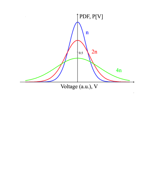
Figure 1:  (Color online) This figure shows the representative probability distribution functions of random voltages arising from the screened potential (13) of randomly distributed charges in an electrically neutral substrate for three different densities (other parameters are fixed).

Due to a complicated structure of the potential in real space, it is not feasible to calculate the full PDF (5) analytically. However, it is easy to perform a numerical evaluation of the corresponding integrals. A result of such calculation is shown in Fig. 1, where representative PDFs are plotted for three different densities. We note that different portions of the curves can be very well-fitted with Gaussians, but the entire dependence is definitely more complicated than a simple Gaussian. Moreover, if $\overline{V}\neq 0$ (a charged substrate), the distribution function is not even symmetric with respect to $\delta V=\left(V-\overline{V}\right)$, i.e. $P[\delta V]\neq P[-\delta V]$.

Even though the full PDF can not be determined analytically, one can evaluate explicitly its moments using Eqs. (9) and (10). In particular, we calculate the second moment for the case of Thomas-Fermi screening, $\overline{\delta V^{2}}=\overline{\left(V-\overline{V}\right)^{2}}$; the result is

$$\overline{\delta V^{2}}=2\pi n_{\rm imp}Q_{0}^{2}\left[{\rm E_{1}}\,(2q_{\rm s}d)e^{2q_{\rm s}d}\left(1+2q_{\rm s}d\right)-1\right],$$ (14)

where $E_{1}(z)=\int_{z}^{\infty}t^{-1}e^{-t}dt$ is the exponential integral function. Obviously, the statistical properties of the potential strongly depend on the parameter $q_{\rm s}d$. Below we give asymptotic expressions for $\overline{\delta V^{2}}$ in the limits of large and small $q_{\rm s}d$

$$\overline{\delta V^{2}}=2\pi n_{\rm imp}Q_{0}^{2}\left\{\begin{array}[]{ll}\left(2q_{\rm s}d\right)^{-2},&\mbox{if }\,q_{\rm s}d\gg 1;\\ \ln{\left[\frac{1}{2e\gamma q_{\rm s}d}\right]},&\mbox{if }\,q_{\rm s}d\ll 1,\end{array}\right.$$ (15)

where $\gamma\approx 1.781$ is the Euler’s constant, $e\approx 2.718$ is the base of the natural logarithm. We note that the last expression essentially reproduces the result obtained above for the bare Coulomb potential [see Eq. (11) and the text below it].

Next we study the correlation function $\langle V({\bf r})V(0)\rangle$, which is related to the typical size of electron/hole puddles. To simplify the notation we define a new function $C(r)$ according to the following relation $\langle V({\bf r})V(0)\rangle=\overline{V}^{2}+2\pi n_{\rm imp}Q_{0}^{2}C(r)$. Using Eq. (10), one can calculate analytically all coefficients in the Taylor series for the correlator $C(r)$

$$C(r)=C_{0}(2q_{\rm s}d)+\sum_{m>0}(-1)^{m}(q_{\rm s}r)^{2m}\frac{(2m-1)!!}{2^{m}m!}C_{m}(2q_{\rm s}d),$$ (16)

where $C_{m}(x)=[1/(2m)!](\partial_{x}^{2m+1})[xe^{x}E_{1}(x)]$. Note that $C_{0}$ reproduces the expression in the square brackets in Eq. (14). In the limit $q_{\rm s}r\ll 1$, the correlator behaves as $C(r)\approx C_{0}-(C_{1}/2)(q_{\rm s}r)^{2}$. In the opposite limit of $q_{\rm s}r\gg 1$, one finds that the correlation function decays as a power law $C(r)\sim 2|1-q_{\rm s}d|(q_{\rm s}r)^{-3}$. The general form of the correlator has been calculated numerically in Sec. V.1 and is shown in Fig 2.

V Application to graphene

V.1 Size of the puddles

Now, we apply the general results obtained above specifically to the case of a graphene sheet in the experimentally relevant parameter regime. We estimate the density of charged impurities, the parameter $q_{\rm s}d$, which determines the behavior of the correlation function $C(r)$, the typical size of a fluctuation-induced electron/hole droplet due to the charge impurity fluctuations, and the typical width of the region where the conductivity is expected to be almost a constant. We estimate these quantities for typical graphene samples with mobilities $\mu\sim 10^{4}\mathrm{cm}^{2}/Vs$. The deviation from the semi-classical Drude-Boltzmann theory occurs at carrier densities $n\sim n_{\mathrm{imp}}\approx 5\times 10^{11}\mathrm{cm}^{-2}$  kn:hwang2006c . This leads to the density of states $\nu_{0}\approx 10^{10}\mathrm{cm}^{-2}\mathrm{meV}^{-1}$ and the Fermi energy $E_{\rm F}\approx 80~{}\mathrm{meV}$. Assuming that the distance between the graphene plane and the substrate is $d\sim 1\mathrm{nm}$, we find $q_{\rm s}d\sim 0.5$. The corresponding correlation function is plotted in Fig. 2. This correlation function determines the size of a disorder-induced puddle, which can be roughly estimated as $l\sim 10\mathrm{nm}$. We also can determine the average value of the random potential as $\overline{V}=n_{\mathrm{imp}}/\nu_{0}\approx 0.05~{}\mathrm{eV}$ and $\sqrt{\overline{\delta V^{2}}}\approx 0.1~{}\mathrm{eV}$. The former number determines the asymmetry in the conductivity dependence, $\sigma(V_{\rm g})$, while the latter estimates the width $\overline{\Delta V_{g}}$ of the constant conductivity plateau. These numbers are in a reasonable agreement with the available experimental data and validate the basic model that the minimum conductivity in graphene is connected with the density inhomogeneities caused by the charged impurities in the $\mathrm{SiO}_{2}$ substrate. We note two direct experimental consequences of our theoretical findings: (1) Dirtier samples should have larger vales of $\Delta V_{g}$; implying higher (lower) mobility samples should have smaller (larger) values of $\Delta V_{g}$. (2) In addition, $\Delta V_{g}$ has a nontrivial dependence on $d$, the impurity location [see, Eq. (15)], which can, in principle, be experimentally verified.

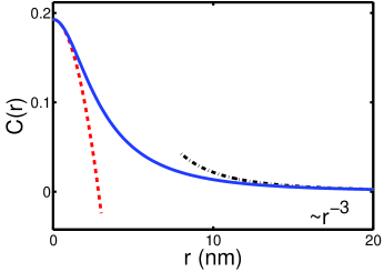
Figure 2:  (Color online) The correlation function $C(r)$ [see Eq. (10) and text for the definition] for the charge impurity model with linear Thomas-Fermi screening. The solid line shows numerical integration for $q_{\rm s}d=0.5$, while the dashed lines correspond to the asymptotic analytical expressions for small and large $q_{\rm s}r$. The chosen value of $q_{\rm s}d=0.5$ is determined by the density of carriers, where the experimentally observed behavior deviates from the predictions of the classical Drude-Boltzmann theory.

While the voltage (or density) width of the residual minimal conductivity regime is explained naturally in our theory of impurity induced inhomogeneous electron-hole puddle picture, getting the exact values of the residual density and the minimal conductivity will require a detailed calculation involving percolation through a network of random 2D electron and hole puddles. Adam et al. (2007); CFAA The following section provides estimates of these quantities in the framework of a self-consistent “mean-field” approach, which should be quantitatively reliable away from the precise percolation point.

V.2 Mean-field approach and relation to diagrammatics

In this section, we briefly outline possible approaches to relate the voltage fluctuations to observables and, in particular, discuss the regime of high gate voltages, where the usual diagrammatic perturbation theory becomes quantitatively applicable and show a possible relation between the discussed charge disorder fluctuation phenomena and the diagrammatic approach. We also formulate here a self-consistent mean-field-like approximation, which allows us to roughly estimate some observable parameters in the regime where perturbation theory breaks down.

While it is intuitively clear that the local voltage fluctuations lead to a non-vanishing density in the two-dimensional plane, the exact relation between the voltage distribution and the density is non-trivial. Generally, one has to solve the many-body Schrödinger equation taking into account the long-range disorder potential and Coulomb interaction between carriers, which is an extremely complicated if not impossible task to accomplish. Efros et al. Efros et al. (1993) have previously formulated a phenomenological approach in which the density is determined from minimization of the energy of the system written in terms of the position-dependent density $\Omega=\int d^{2}r\left\{\frac{1}{2}V({\bf r})\left[n({\bf r})-\overline{n}\right]+E[n({\bf r})]\right\}$, where the first term describes the Coulomb interaction between the impurity charges and the induced carriers and the local density, while the second term represents the energy of a uniform liquid (which includes the kinetic and exchange correlation effects). Formally, this approach would allow to interpolate between the regimes of large and small carrier density; but in the former case, i.e., if the chemical potential is large, the effect of charge disorder fluctuations is a small perturbation and the aforementioned phenomenological approach should reduce to the usual microscopic perturbation theory. E.g., one can determine the relevant density-density correlation function $\left\langle\delta n({\bf r})\delta n({\bf r}^{\prime})\right\rangle)$ by considering diagrams in Fig. 3a, where the dashed line represents the electron scattering off of the Coulomb impurity potential and the shaded vertices imply a ladder of such charge impurity lines. We note that to avoid infrared divergencies, one has to consider screening of the impurity potential by carriers, $U({\bf r},{\bf r}^{\prime})=v({\bf r}-{\bf r}^{\prime})+[v*\Pi*U]({\bf r},{\bf r}^{\prime})$ (where $v$ is the bare potential and $\Pi$ is a polarization operator). Strictly speaking, the screening properties and the interaction between two charges are random quantities themselves, which depend on the positions of the charges. In particular, the polarization operator, which determines the screening properties is a random matrix, $\Pi({\bf r},{\bf r}^{\prime})$, which depends on two coordinates. The probability distribution function of this matrix (in the Gaussian approximation) is a functional $F[\delta\Pi]=\exp\left[-(1/2)\int_{1,2,3,4}\delta\Pi(1,2)C^{-1}(1,2;3,4)\delta\Pi(1,2)\right]$, where $C^{-1}(1,2;3,4)$ is the inverse correlator $\langle\delta\Pi({\bf r}_{1},{\bf r}_{2})\delta\Pi({\bf r}_{3},{\bf r}_{4})\rangle$, which is described by the diagrams in Fig. 3b. Clearly in the high-density regime, the average screening length $q_{s}^{-1}$ will be determined just by the average density, with small “mesoscopic” corrections. Similarly in this regime, where the Fermi wave-length is the smallest length scale in the problem, the local density in a particular point will be determined just by the local voltage which can be viewed as a local chemical potential in this point. Therefore, the average density fluctuation (up to a numerical constant of order one) should be of the order of $\sqrt{\langle(n-\overline{n})^{2}\rangle}\sim n(\mu\sim\sqrt{\overline{\delta V^{2}}})$ [where $n(\mu)$ is the dependence of the density on the chemical potential in the uniform case and $\overline{\delta V^{2}}$ is given by (14)].

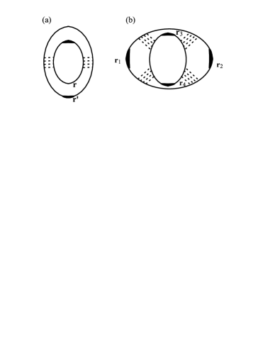
Figure 3:  Fig. 3a is the pictorial representation of the disorder-induced density fluctuations $\left\langle\delta n({\bf r})\delta n({\bf r}^{\prime})\right\rangle$, where the dashed line represents the Coulomb impurity potential and the shaded vertex is a ladder of these impurity lines. Fig. 3b is a diagram, which contributes to the correlator $\langle\delta\Pi({\bf r}_{1},{\bf r}_{2})\delta\Pi({\bf r}_{3},{\bf r}_{4})\rangle$ of the polarization operators, which determine the screening properties and the effective interaction (see text).

When the external gate voltage and thus the chemical potential and the Fermi-momentum decrease, the microscopic perturbation theory of density fluctuations in graphene breaks down. The Green’s functions and the screening properties of the impurity potential in Fig. 3 both depend on the average density, which vanishes at the Dirac point and the corresponding computation becomes ill-defined. However, it is possible to formulate a reasonable and simple self-consistent scheme, which would allow to get an order-of-magnitude estimate of the density in the vicinity of the Dirac point. Namely, one assumes that the Green’s functions and the screening length correspond to a uniform density $\sim\sqrt{\overline{\delta^{2}n}}$. Then, using these objects one can calculate the density fluctuation, which, as argued above, should be of order

$$\sqrt{\overline{\delta^{2}n}}\sim n(\mu\sim\sqrt{\overline{\delta V^{2}}}).$$

But in this equation, the right hand-side of this relation itself depends on $\overline{\delta^{2}n}$ via the screening length $q_{s}^{-1}$ [see, Eq. (14) of Sec. IV]. This leads to an algebraic non-linear self-consistency equation for the typical density fluctuation. The corresponding calculation has been done by us and is described in detail in Ref. [Adam et al., 2007] (the corresponding estimate for the residual density is $n\sim 0.1-1n_{\rm imp}$).

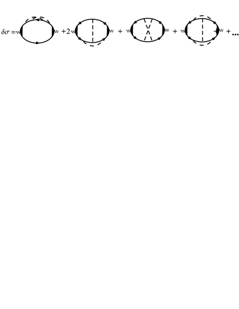
Figure 4:  The first few diagrams in the perturbative expansion of the conductivity. The dashed lines correspond to the scattering off of Coulomb disorder potential.

A more important experimentally measurable quantity is the conductivity. At very high gate voltages, the usual semiclassical Drude-Boltzmann theory works perfectly well. As the chemical potential is lowered, the “mesoscopic fluctuation” effects start to appear. In the regime, when these effects are a small correction to the classical conductivity, one should be able to obtain them in the framework of the conventional diagrammatic technique. This implies going beyond the Drude approximation (no crossed impurity lines) and calculating “quantum corrections” to the conductivity. A formal calculation would select the maximally crossed weak-localization diagram, which diverges in the zero-temperature limit. However, the flattening of the linear-in-$V$ conductivity most likely has nothing to do with the weak localization or any other quantum interference effect of this type. The effect of minimum conductivity is “quantum” only in the sense that diagrammatically it appears beyond the classical Drude approximation and is due to diagrams with some crossed impurity lines. We note that in the case of long-range Coulomb disorder, there are other dimensionless parameters apart from $k_{F}l$ (namely, $r_{s}$ which formally should be assumed small for perturbation theory to hold). If the dephasing time is short enough, other types of diagrams (e.g., impurity vertex corrections) may be more important than the weak localization diagram. We believe that in the recent experiments, which observed the minimum conductivity, the latter scenario is realized. The fate of the weak localization correction is a very interesting but separate question, which seems to be irrelevant to the effect of the flattening of conductivity at low gate voltages. The initial deviation of the $\sigma(V_{g})$-dependence from the straight line can be obtained from the usual perturbation theory by considering just the next-to-leading diagrams with a finite number of crossed Coulomb impurity lines (see Figs. 4b and 4c). The corresponding calculation will be published elsewhere.

As noted above, in the limit of zero or very small gate voltage (in the very vicinity of the Dirac point), the microscopic perturbation theory breaks down and only qualitative descriptions are available. In this regime, transport occurs via a percolation network of electron and hole puddles. Cheianov et al. CFAA recently proposed a random resistor network model and calculated a scaling behavior of the conductivity near the percolation threshold. While the corresponding scaling function may be universal, the value of the minimal conductivity itself is non-universal (e.g., it depends on the choice of the underlying lattice) and can not be determined within a random resistance network model. The possibility that disorder associated with random charged impurities could lead to a non-universal graphene minimum conductivity was pointed out in Ref. [kn:hwang2006c, ], and the value of the minimal conductivity was estimated in Ref. [Adam et al., 2007], by assuming that it is of the order of Drude-Boltzmann conductivity with the density determined by the value of the typical density obtained via the self-consistent procedure explained above. We note that this estimate agrees very well with the available experimental data Tan et al. (2007) (e.g., both the high-voltage Drude behavior and the minimal conductivity can be determined using just one fitting parameter - the density of impurities in the substrate).

VI Conclusion

In this paper, we developed a simple and general method of calculating statistical properties of voltage fluctuations due to charge disorder in the vicinity of a conducting two-dimensional plane. We used these results to describe the low-density properties of a graphene sheet near a substrate with Coulomb impurities. In particular, we estimated the typical size of the electron and hole puddles and the width of the minimum conductivity plateau. We also proposed a self-consistent approximation scheme to estimate the typical residual density and conductivity at the Dirac point. The corresponding results appear to be in a good agreement with experimental data. Tan et al. (2007)

While our theory based on density fluctuations by extrinsic charged impurities invariably present in the substrate provides a reasonable mean-field description of the observed graphene non-universal conductivity minimum plateau around the charge neutrality point, an important open question remains on the transport behavior precisely at the percolation critical point $V_{g}=V_{c}$ where infinite electron and hole percolation paths open for transport throughout the system. Neither the mean-field theory of Ref. [Adam et al., 2007] nor the perturbative diagrammatic approach can qualitatively access the critical point where the density fluctuations are very large. Unfortunately, the problem of determining the minimum conductivity at $V_{c}$ remains inaccessible to the theory. We should mention that recently Cheianov et al. CFAA studied the critical percolation problem by effectively including tunneling between the neighboring electron/hole puddles within a lattice random-resistance model, however their numerical analysis has not led to any estimate of the non-universal non-universal conductivity at the percolation critical point. Experiment seems to indicate a smooth and continuous behavior as one goes from the $V_{g}<V_{c}$ to the $V_{g}>V_{c}$ regime with the minimum conductivity remaining approximately a constant over a finite interval of voltage $\delta V_{g}$, i.e. in the regime $V_{g}-\delta V_{g}<V_{c}<V_{g}+\delta V_{g}$, as the voltage swept through the charge neutrality point. The “mean-field theory” seems to provide a reasonable quantitative estimate of both $\sigma_{\rm min}\sim\sigma(V_{c})$ and the value of $\delta V_{g}$ itself as well as the conductivity $\sigma(|V_{g}|)\gg|V_{c}|$ far from the electron-hole puddle percolation regime. Whether there is some remnant universal quantum conductivity behavior, arising from the special quantum-mechanical properties of the chiral Dirac-like graphene band dispersion, remains an important open question. The smooth and continuous experimental behavior of graphene transport through the charge neutrality point empirically argues against any universal behavior, but we can not rule it out on the current theoretical grounds. In fact, closely connected with the critical percolation transport is the question of (the absence of any observed) Anderson localization in graphene. The strong disorder associated with the random charged impurities should lead to strong Anderson localization in graphene. Experimentally, however, no such strong localization effect has ever been seen in graphene and even the most disordered graphene samples seem to have a finite minimum conductivity which is relatively temperature independent around $T\lesssim 100$ mK. Why this is so is not understood theoretically. It is possible that the crossover to strong localization occurs at very low temperatures but more experimental and theoretical work is needed to settle this important question. The issues of the critical percolation transport near the charge neutrality point and the apparent absence of Anderson localization in graphene are both beyond the scope of this work.

An important conclusion, which follows from our work is that there will be no percolation induced metal-insulator transition in graphene as there is in 2D semiconductor systems Das Sarma et al. (2005) and the graphene layer will always conduct at low density (leading to a residual conductivity), as long as there is no Anderson localization, simply because the electron and hole percolation densities are exactly equal by duality in two dimensions, and therefore, either the electron or the hole channel always conducts independent of how strong the impurity-induced inhomogeneous voltage fluctuations are. This residual conductivity is not universal and depends on the density of charge impurities.

Finally, we emphasize that the theoretical technique we develop in this paper for calculating the non-Gaussian probability distribution function of charged impurity induced voltage fluctuations is completely general, and can be used for other 2D systems, e.g. modulation-doped semiconductor heterostructures and quantum wells, where such fluctuation-induced density inhomogeneity and puddle formation effects Das Sarma et al. (2005) are known to be important, often leading to percolation-induced conductor-to-insulator transition. We believe that the theoretical framework developed in this work can be adapted to 2D disordered semiconductors providing insight into the nature of transport in these systems.

Note added: After the first version of this manuscript had been submitted, we received a preprint kn:martin2007 , which reported an explicit experimental observation of the electron-hole puddles in graphene and provided an estimate of a puddle size in quantitative agreement with our theory. Acknowledgements: This work is supported by US-ONR.

References

- Efros et al. (1993) A. L. Efros, F. G. Pikus, and V. G. Burnett, Phys. Rev. B 47, 2233 (1993); B. I. Shklovskii and A. L. Efros, Electronic Properties of Doped Semiconductors (Springer, New York, 1984).
- Novoselov et al. (2004) K. S. Novoselov, A. K. Geim, S. V. Morozov, D. Jiang, Y. Zhang, S. V. Dubonos, I. V. Grigorieva, and A. A. Firsov, Science 306, 666 (2004).
- Novoselov et al. (2005) K. S. Novoselov, A. K. Geim, S. V. Morozov, D. Jiang, Y. Zhang, M. I. Katsnelson, I. V. Grigorieva, S. V. Dubonos, and A. A. Firsov, Nature 438, 197 (2005).
- Zhang et al. (2005) Y. Zhang, Y.-W. Tan, H. L. Stormer, and P. Kim, Nature 438, 201 (2005).
- (5) E. H. Hwang, S. Adam, and S. Das Sarma, Phys. Rev. Lett 98, 186806 (2007); and arXiv:cond-mat/0610834 (2006).
- Nomura and MacDonald (2006) K. Nomura and A. H. MacDonald, Phys. Rev. Lett. 96, 256602 (2006); V. V. Cheianov and V. I. Fal’ko, Phys. Rev. Lett. 97, 226801 (2006).
- Fradkin (1986) E. Fradkin, Phys. Rev. B 33, 3257 (1986); A. W. W. Ludwig, M. P. A. Fisher, R. Shankar, and G. Grinstein, Phys. Rev. B 50, 7526 (1994).
- Katsnelson (2006) M. I. Katsnelson, Eur. Phys. J. B 51, 157 (2006); J. Tworzydło, B. Trauzettel, M. Titov, A. Rycerz, and C. W. J. Beenakker, Phys. Rev. Lett. 96, 246802 (2006).
- (9) J. A. Nixon and J. H. Davis, Phys. Rev. B 41, 7929 (1990).
- (10) B. Huard, J.A. Sulpizio, N. Stander, K. Todd, B. Yang, and D. Goldhaber-Gordon, Phys. Rev. Lett. 98, 236803 (2007).
- Adam et al. (2007) S. Adam, E. H. Hwang, V. M. Galitski, and S. Das Sarma, Proc. Natl. Acad. Sci. USA, in press (arXiv:0705.1540 [cond-mat.mes-hall]) (2007).
- (12) V.V. Cheianov, V.I. Falko, B.L. Altshuler, and I.L. Aleiner, Phys. Rev. Lett 99, 176801 (2007); and arXiv:0706.2968 (2007).
- Tan et al. (2007) Y.-W. Tan, Y. Zhang, K. Bolotin, Y. Zhao, S. Adam, E. H. Hwang, S. Das Sarma, H. L. Stormer, and P. Kim, Phys. Rev. Lett. in press (arXiv:0707.1807v1 [cond-mat.mes-hall]) (2007).
- Larkin et al. (1971) A. I. Larkin, V. Mel’nikov, and D. Khmelnitskii, Zh. Eksp. Teor. Fiz. 60, 846 (1971), [Sov. Phys. JETP 33, 458 (1971)]; V. M. Galitski and A. I. Larkin, Phys. Rev. B 66, 064526 (2002).
- Das Sarma et al. (2005) S. Das Sarma, M. P. Lilly, E. H. Hwang, L. N. Pfeiffer, K. W. West, and J. L. Reno, Phys. Rev. Lett. 94, 136401 (2005).
- (16) J. Martin, N. Akerman, G. Ulbricht, T. Lohmann, J. H. Smet, K. von Klitzing, and A. Yacoby, arXiv:0705.2180 (2007).