Present address: ]20 Antrim Crescent, Apt. 1412, Scarborough, Ontario M1P 4N3, Canada

Nature of the Bogoliubov ground state of a weakly interacting Bose gas

Abstract

As is well-known, in Bogoliubov’s theory of an interacting Bose gas the ground state of the Hamiltonian $\hat{H}=\sum_{\bf k\neq 0}\hat{H}_{\bf k}$ is found by diagonalizing each of the Hamiltonians $\hat{H}_{\bf k}$ corresponding to a given momentum mode ${\bf k}$ independently of the Hamiltonians $\hat{H}_{\bf k^{\prime}(\neq k)}$ of the remaining modes. We argue that this way of diagonalizing $\hat{H}$ may not be adequate, since the Hilbert spaces where the single-mode Hamiltonians $\hat{H}_{\bf k}$ are diagonalized are not disjoint, but have the ${\bf k}=0$ in common. A number-conserving generalization of Bogoliubov’s method is presented where the total Hamiltonian $\hat{H}$ is diagonalized directly. When this is done, the spectrum of excitations changes from a gapless one, as predicted by Bogoliubov’s method, to one which has a finite gap in the $k\to 0$ limit.

Introduction. Since its inception in 1947, Bogoliubov’s approach to interacting Bose systems Bogoliubov1947 has been one of the most influential theories in condensed matter physics. Lee1957 ; LeeHuangYang1957 ; Bruckner1957 ; Beliaev1958 ; Hugenholtz1959 ; Sawada1959 ; Gavoret1964 ; Hohenberg1965 ; Popov1965 ; Singh1967 ; Cheung1971 ; Szepfalusy1974 Yet, for all its notoriety and popularity within the physics community, a key aspect of this theory, having to do with the decoupled way in which the Hamiltonian is diagonalized, is still not fully understood. Indeed, and as is well-known, in the standard formulation of Bogoliubov’s theory, the Hamiltonian $\hat{H}$ is written as a decoupled sum of contributions from different momenta of the form $\hat{H}=\sum_{\bf k\neq 0}\hat{H}_{\bf k}$, where each Hamiltonian $\hat{H}_{\bf k}$ describes the interaction of bosons in the condensed $\bf k=0$ state with bosons in the momentum modes $\pm\bf k$, then each of the single-mode Hamiltonians $\hat{H}_{\bf k}$ is diagonalized separately and the ground state (GS) wavefunction of $\hat{H}$ is written as the product of the GS wavefunctions of the $\hat{H}_{\bf k}$’s. In this letter, we shall argue that, while this way of diagonalizing the total Hamiltonian $\hat{H}$ may seem to be valid from the perspective of the standard, number non-conserving Bogoliubov’s method, where the $\bf k=0$ state is removed from the Hilbert space and hence the individual Hilbert spaces where the Hamiltonians $\{\hat{H}_{\bf k}\}$ are diagonalized are disjoint with one another, from a number-conserving perspective this diagonalization method may not be adequate since the true Hilbert spaces where the Hamiltonians $\{\hat{H}_{\bf k}\}$ should be diagonalized all have the ${\bf k}=0$ state in common. We then shall discuss a variational, number-conserving generalization of Bogoliubov’s theory in which the ${\bf k}=0$ state is restored into the Hilbert space of the interacting gas, and where, instead of diagonalizing the Hamiltonians $\hat{H}_{\bf k}$ separately, we diagonalize the total Hamiltonian $\hat{H}$ as a whole. When this is done, the spectrum of excitations of the system changes from a gapless one, as predicted by the standard, number non-conserving Bogoliubov method, to one which exhibits a finite gap in the $k\to 0$ limit.

Variational formulation of Bogoliubov’s theory. We shall start by discussing a variational formulation LeeHuangYang1957 ; LeggettRMP of Bogoliubov’s theory which, historically, has constituted the basis of the justification of the number non-conserving formulation of this method. As is well-known, in Bogoliubov’s approach one only retains in the total Hamiltonian $\hat{H}$ of the system (i) kinetic energy terms of the form $\sum_{\bf k\neq 0}\varepsilon_{\bf k}a_{\bf k}^{\dagger}a_{\bf k}$, (ii) Hartree terms $\sum_{\bf k,k^{\prime}}v({\bf 0})a_{\bf k}^{\dagger}a_{\bf k^{\prime}}^{\dagger}a_{\bf k}a_{\bf k^{\prime}}/2V$, (iii) Fock terms $\sum_{\bf k\neq 0}v({\bf k})a_{\bf k}^{\dagger}a_{\bf k}a_{\bf 0}^{\dagger}a_{\bf 0}/V$ describing the exchange interaction between condensed bosons and depleted ones, and (iv) pairing terms of the form $\sum_{\bf k\neq 0}v({\bf k})(a_{0}a_{0}a_{\bf k}^{\dagger}a_{-\bf k}^{\dagger}+a_{0}^{\dagger}a_{0}^{\dagger}a_{\bf k}a_{-\bf k})/2V$. (In the above expressions, $\varepsilon_{\bf k}=\hbar^{2}k^{2}/2m$ is the kinetic energy of a boson of mass $m$ and wavevector ${\bf k}$, $v({\bf k})$ is the Fourier transform of the interaction potential between bosons, and $V$ is the volume of the system. On the other hand, $a_{\bf k}^{\dagger}$ and $a_{\bf k}$ are creation and annihilation operators, respectively). Considering that we will be focusing on systems having a fixed number of particles $N$, it is convenient to take the origin of energies at the Gross-Pitaevskii value $v(0)N(N-1)/2V$. Then it can be shown LeggettRMP that the Hamiltonian can be written as a sum of independent contributions from different values of ${\bf k}$ of the form $\hat{H}\simeq\sum_{\bf k\neq 0}\hat{H}_{\bf k}$, where (throughout this paper, for all explicit calculations we shall be using the interaction potential $v({\bf r})=g\delta({\bf r})$, for which $v({\bf k})=g$):

$$\hat{H}_{\bf k}=\varepsilon_{\bf k}a_{\bf k}^{\dagger}a_{\bf k} +\frac{v({\bf k})}{2V}\,\big{(}2a_{0}^{\dagger}a_{0}a_{\bf k}^{\dagger}a_{\bf k}$$

$$+a_{\bf k}^{\dagger}a_{-\bf k}^{\dagger}a_{0}a_{0}+a_{0}^{\dagger}a_{0}^{\dagger}a_{\bf k}a_{-\bf k}\big{)}.$$ (1)

We now proceed to diagonalize the Hamiltonian $\hat{H}_{\bf k}$ by considering a hypothetical system where bosons are only allowed to be in one of the three single particle states with momentum ${\bf k}$, ${\bf 0}$ or $-\bf k$. In order to formulate a variational approach for the Hamiltonian $\hat{H}_{\bf k}$ describing such a system, it is sufficient to restrict our attention to the Hilbert space ${\cal H}_{\bf k}$ spanned by kets $|n\rangle$ of the form:

$$|n\rangle\equiv|N-2n,n,n\rangle=\frac{(a_{0}^{\dagger})^{N-2n}}{\sqrt{(N-2n)!}}\frac{(a_{\bf k}^{\dagger})^{n}}{\sqrt{n!}}\frac{(a_{-\bf k}^{\dagger})^{n}}{\sqrt{n!}}|0\rangle,$$ (2)

having $n$ bosons with momentum ${\bf k}$ and momentum $-{\bf k}$, and $N-2n$ bosons in the ${\bf k}={\bf 0}$ state. The general expression of the GS wavefunction $|\psi_{\bf k}\rangle$ of the Hamiltonian $\hat{H}_{\bf k}$ in this Hilbert space is given by $|\psi_{\bf k}\rangle=\sum_{n=0}^{N/2}C_{n}|n\rangle$, and it can easily be verified that the expectation value of $\hat{H}_{\bf k}$ in the state $|\psi_{\bf k}\rangle$ can be written in the form:

$$\langle\psi_{\bf k}|\hat{H}_{\bf k}|\psi_{\bf k}\rangle=\sum_{n=0}^{N/2}\Big{\{}|C_{n}|^{2}\Big{[}n\varepsilon_{\bf k}+\frac{v(k)}{V}n(N-2n)\Big{]}$$

$$+\frac{v(k)}{2V}nC_{n}^{*}C_{n-1}\sqrt{(N-2n+2)(N-2n+1)}$$

$$+\frac{v(k)}{2V}(n+1)C_{n}^{*}C_{n+1}\sqrt{(N-2n-1)(N-2n)}\Big{\}},$$ (3)

where it is understood that $C_{-1}=C_{1+(N/2)}=0$. Assuming, for simplicity, that the coefficients $C_{n}$ are real, it follows that, for $v(k)>0$, the expectation value $\langle\psi_{\bf k}|\hat{H}_{\bf k}|\psi_{\bf k}\rangle$ will be lowered if the coefficients $C_{n}$ have alternating positive and negative signs. In this case, the terms on the second and third line will be negative, making the expectation value lower than what one would obtain if products of the form $C_{n}C_{n-1}$ and $C_{n}C_{n+1}$ are positive. Bogoliubov’s theory corresponds to a variational ansatz in which the coefficients $C_{n}$ are assumed to be of the form $C_{n}=(-c_{\bf k})^{n}$, where the constant $c_{\bf k}>0$ is to be determined variationally. The coefficients $C_{n}$ are expected to decrease with $n$, which encodes the fact that the probability amplitude of states $|n\rangle$ with a large number $n\gg 1$ of bosons having a wavevector $\pm{\bf k}$ will be small. This implies that the constant $c_{\bf k}$ must be less than unity.

Inserting the variational ansatz $C_{n}=(-c_{\bf k})^{n}$ into Eq. (3), and making use of the approximation $\sqrt{N(N+1)}\simeq N+\frac{1}{2}$ which is valid for $N\gg 1$, we can write:

$$\langle\psi_{\bf k}|\hat{H}_{\bf k}|\psi_{\bf k}\rangle\simeq\sum_{n=0}^{N/2}\Big{\{}(c_{\bf k})^{2n}\big{[}n\varepsilon_{\bf k}+\frac{v(k)}{V}n(N-2n)\big{]}$$

$$+\frac{v(k)}{2V}n(c_{\bf k})^{2n-1}\Big{(}N-2n+\frac{3}{2}\Big{)}$$

$$+\frac{v(k)}{2V}(n+1)(c_{\bf k})^{2n+1}\Big{(}N-2n-\frac{1}{2}\Big{)}\Big{\}}.$$ (4)

The summations in the above equation can be calculated analytically by taking successive derivatives with respect to the variable $x$ of the result $\sum_{n=0}^{N/2}x^{n}\simeq 1/(1-x)$, valid for $|x|<1$ and $N\to\infty$, hence obtaining:

$$\sum_{n=1}^{N/2}nx^{n}\simeq\frac{x}{(1-x)^{2}},\quad\sum_{n=1}^{N/2}n^{2}x^{n}\simeq\frac{x+x^{2}}{(1-x)^{3}}.$$ (5)

Using these last two results in Eq. (4), we obtain:

$$\langle\psi_{\bf k}|\hat{H}_{\bf k}|\psi_{\bf k}\rangle=\frac{c_{\bf k}}{(1-c_{\bf k}^{2})^{2}}\Big{[}c_{\bf k}\varepsilon_{\bf k}+v(k)n_{B}\big{(}c_{\bf k}-1\big{)}\Big{]},$$ (6)

where we denote by $n_{B}=N/V$ the density of bosons in the system. On the other hand, from the definition of $|\psi_{\bf k}\rangle$, we easily see that the norm of the wavefunction $\langle\psi_{\bf k}|\psi_{\bf k}\rangle$ is given by $\langle\psi_{\bf k}|\psi_{\bf k}\rangle=\sum_{n=0}^{N/2}|C_{n}|^{2}\simeq 1/(1-c_{\bf k}^{2})$. Now, if we divide Eq. (6) by this last expression of $\langle\psi_{\bf k}|\psi_{\bf k}\rangle$, we can write for the normalized expectation value $\langle\hat{H}_{\bf k}\rangle_{\bf k}=\langle\psi_{\bf k}|\hat{H}_{\bf k}|\psi_{\bf k}\rangle/\langle\psi_{\bf k}|\psi_{\bf k}\rangle$ the following result:

$$\langle\hat{H}_{\bf k}\rangle_{\bf k}\simeq\frac{c_{\bf k}^{2}}{1-c_{\bf k}^{2}}\big{[}\varepsilon_{\bf k}+v(k)n_{B}\big{]}-v(k)n_{B}\frac{c_{\bf k}}{1-c_{\bf k}^{2}}.$$ (7)

Minimization of the above expectation value with respect to $c_{\bf k}$ leads to the quadratic equation $c_{\bf k}^{2}-2\left(\frac{\cal{E}_{\bf k}}{v(k)n_{B}}\right)c_{\bf k}+1=0$, where we defined ${\cal{E}_{\bf k}}=\varepsilon_{\bf k}+v(k)n_{B}$. The above quadratic equation has two roots, of which only one satisfies the constraint $0<c_{\bf k}<1$ for arbitrary values of ${\cal E}_{\bf k}$. This root is given by:LeggettRMP

$$c_{\bf k}=\frac{1}{v(k)n_{B}}\left[{\cal E}_{\bf k}-\sqrt{{\cal E}_{\bf k}^{2}-v(k)^{2}n_{B}^{2}}\right].$$ (8)

This result for the constant $c_{\bf k}$ fully determines the coeffcients $C_{n}=(-c_{\bf k})^{n}$ of the variational ground state $|\psi_{\bf k}\rangle$ of the Hamiltonian $\hat{H}_{\bf k}$. The coefficients $\widetilde{C}_{n}=C_{n}\sqrt{1-c_{\bf k}^{2}}$ of the normalized wavefunction $|\widetilde{\psi}_{\bf k}\rangle=|\psi_{\bf k}\rangle/\sqrt{\langle\psi_{\bf k}|\psi_{\bf k}\rangle}$ are plotted (as the crosses) in Fig. 1 for $\tilde{k}=0.1$ in dimensionless units such that $\tilde{k}\equiv\hbar k/\sqrt{2mv(0)n_{B}}$. The circles in this last figure are the coefficients obtained by direct numerical diagonalization of the Hamiltonian $\hat{H}_{\bf k}$. It is seen that there is a pretty good agreement between the results of our variational method and the exact numerical diagonalization for the particular value of $k$ chosen.

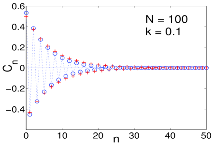
Figure 1: Coefficients $\widetilde{C}_{n}$ of the normalized wavefunction $|\widetilde{\psi}_{\bf k}\rangle$ for $N=100$ bosons and $\tilde{k}=0.1$. The crosses are the results of Bogoliubov’s theory, and the circles are the results of the exact numerical diagonalization of the Hamiltonian $\hat{H}_{\bf k}$.

The expectation value of $\hat{H}_{\bf k}$ in the ground state $|\psi_{\bf k}\rangle$ can readily be found if we use the result (8) for $c_{\bf k}$ in Eq. (7), upon which we obtain:

$$\langle\hat{H}_{\bf k}\rangle_{\bf k}=\frac{1}{2}\Big{[}\sqrt{\varepsilon_{\bf k}\big{[}\varepsilon_{\bf k}+2n_{B}v(k)\big{]}}-\varepsilon_{\bf k}-n_{B}v(k)\Big{]}.$$ (9)

The result (9) is exactly what one obtains in the standard, number non-conserving Bogoliubov approach for the expectation value of a given contribution $\hat{H}_{\bf k}$ to the Bogoliubov ground state energy. This agrees with the well-known fact that Bogoliubov’s theory is a theory in which the Hamiltonians $\hat{H}_{\bf k}$ are diagonalized independently from one another in essentially disjoint Hilbert spaces. Indeed, the quantity in Eq. (9) is nothing but the expectation value $\langle\widetilde{\psi}_{\bf k}(N)|\hat{H}_{\bf k}|\widetilde{\psi}_{\bf k}(N)\rangle$, where $|\widetilde{\psi}_{\bf k}(N)\rangle$ is the normalized ground state of the single momentum mode Hamiltonian $\hat{H}_{\bf k}$. The reason such a result is obtained is because in the standard formulation of Bogoliubov’s theory, $a_{0}$ and $a_{0}^{\dagger}$ are replaced by the c-number $\sqrt{N}$. This implies that the commutators $[\hat{H}_{\bf k},\hat{H}_{\bf k^{\prime}}]$ vanish identically for ${\bf k}\neq{\bf k^{\prime}}$, which allows the ground state wavefunction $|\Psi_{B}(N)\rangle$ of the total Hamiltonian $\hat{H}$ to be written as a product of the ground state wavefunctions for each of the Hamiltonians $\hat{H}_{\bf k}$ LeeHuangYang1957 ($M$ here denotes the total number of momentum modes kept in the calculation, which can eventually be taken to infinity):

$$|\Psi_{B}(N)\rangle\equiv\sum_{n_{1}=0}^{\infty}\ldots\sum_{n_{M}=0}^{\infty}\widetilde{C}_{n_{1}}\widetilde{C}_{n_{2}}\cdots\widetilde{C}_{n_{M}}|n_{1};\ldots;n_{M}\rangle,$$

$$\mbox{with}\quad|n_{1};\ldots;n_{M}\rangle=\prod_{i=1}^{M}\frac{\big{(}a_{{\bf k}_{i}}^{\dagger})^{n_{i}}}{\sqrt{n_{i}!}}\frac{\big{(}a_{{-\bf k}_{i}}^{\dagger})^{n_{i}}}{\sqrt{n_{i}!}}|0\rangle.$$ (10)

Here, we would like to emphasize that the above expression of the wavefunction $|\Psi_{B}(N)\rangle$ is only consistent with the variational constants given in Eq. (8) when the ${\bf k}=0$ state is removed from the Hilbert space, with $a_{0}$ and $a_{0}^{\dagger}$ being replaced with $\sqrt{N}$. This means that the ground state wavefunction of Eq. (10) above, despite the appearance of the contrary, corresponds to a number non-conserving approach. A major question that arises is to know how the above result will change if we restore the ${\bf k}=0$ state to the Hilbert space, and if instead of diagonalizing each of the Hamiltonians $\hat{H}_{\bf k}$ separately, we diagonalize $\hat{H}$ directly. This will be done next.

Variational approach for the full Hamiltonian $\hat{H}$. We now want to generalize the variational treatment of the single-mode Hamiltonian $\hat{H}_{\bf k}$ to treat the full Hamiltonian $\hat{H}=\sum_{\bf k\neq 0}\hat{H}_{\bf k}$ of the interacting Bose system. To this end, we shall use for $|\Psi(N)\rangle$ the expression:

$$|\Psi(N)\rangle =\sum_{n_{1}=0}^{\infty}\ldots\sum_{n_{M}=0}^{\infty}\widetilde{C}_{n_{1}}\widetilde{C}_{n_{2}}\ldots\widetilde{C}_{n_{M}}$$

$$\times|N-2\sum_{i=1}^{M}n_{i};n_{1};\ldots;n_{M}\rangle,$$ (11)

where the normalized basis wavefunctions are given by (compare with Eq. (10) of the single-mode theory):

$$|N-2\sum_{i=1}^{M}n_{i}; n_{1};\ldots;n_{M}\rangle=\frac{\big{(}a_{0}^{\dagger}\big{)}^{N-2\sum_{i=1}^{M}n_{i}}}{\sqrt{[N-2\sum_{i=1}^{M}n_{i}]!}}$$

$$\times\prod_{i=1}^{M}\frac{\big{(}a_{{\bf k}_{i}}^{\dagger})^{n_{i}}}{\sqrt{n_{i}!}}\frac{\big{(}a_{{-\bf k}_{i}}^{\dagger})^{n_{i}}}{\sqrt{n_{i}!}}|0\rangle.$$ (12)

Note that the GS wavefunction in Eq. (11) is not a simple product of GS wavefunctions for the single-mode Hamiltonians $\hat{H}_{\bf k}$, and that, even though the expression of these single-mode Hamiltonians $\hat{H}_{\bf k}$ are decoupled and commute with one another, the presence of all the $n_{i}$’s in the number of condensed bosons $\big{[}N-2\sum_{i=1}^{M}n_{i}\big{]}$ acts like an implicit and rather nontrivial coupling between all these Hamiltonians. One can now show Ettouhami that the expectation value $\langle\hat{H}_{{\bf k}_{j}}\rangle$ of the Hamiltonian $\hat{H}_{{\bf k}_{j}}$ in the state $|\Psi(N)\rangle$ is no longer given by Eq. (7), but by the following expression:

$$\langle\hat{H}_{{\bf k}_{j}}\rangle\simeq\frac{c_{{\bf k}_{j}}}{1-c_{{\bf k}_{j}}^{2}}\Big{\{}c_{{\bf k}_{j}}\Big{[}\varepsilon_{{\bf k}_{j}}+\bar{v}(k_{j})n_{B}\Big{]}-\bar{v}(k_{j})n_{B}\Big{\}},$$ (13)

where $\bar{v}(k_{j})$ is given by:

$$\bar{v}(k_{j})\simeq v(k_{j})\Big{(}1-\frac{1}{N}\sum_{\bf k\neq 0}\frac{c_{{\bf k}}^{2}}{1-c_{{\bf k}}^{2}}\Big{)}.$$ (14)

If it were not for the term between parenthesis in this last equation, the result in Eq. (13) would be perfectly identical to the expectation value obtained within the single-mode approach, Eq. (7). It can be shown Ettouhami that minimization of the trial ground state energy given in Eq. (13) over the constants $c_{\bf k}$ leads to a solution of the form:

$$c_{\bf k}=1+C_{d}^{-1}(\tilde{k}^{2}+\tilde{\sigma})-\sqrt{\big{[}1+C_{d}^{-1}(\tilde{k}^{2}+\tilde{\sigma})\big{]}^{2}-1}.$$ (15)

where the constant $\tilde{\sigma}$ is obtained by solving a non-linear self-consistency equation obtained from the minimization procedure, Ettouhami and $C_{d}=1-N_{d}/N$, with $N_{d}=\sum_{\bf k\neq 0}c_{\bf k}^{2}/(1-c_{\bf k}^{2})$ the total number of depleted bosons. To fix ideas, we shall henceforth consider an interacting Bose gas in the dilute limit, and fix the parameter $n_{B}a^{3}$ to be $n_{B}a^{3}=10^{-3}$ ($a$ here being the scattering length, which is related to the interaction strength $g$ through the relation $g={4\pi a\hbar^{2}}/{m}$). For this particular value of $n_{B}a^{3}$, we find $\tilde{\sigma}=0.39$ and $C_{d}=0.9762$. In order to show that these values of $\tilde{\sigma}$ and $C_{d}$ do indeed correspond to a lower energy than what one would obtain by using the coefficients $c_{\bf k}$ of the single-mode theory from Eq. (8) in Eq. (13), in Fig. 2 we plot the product $\tilde{k}^{2}\langle\Psi(N)|\hat{H}_{\bf k}|\Psi(N)\rangle$, which appears in the evaluation of the ground state energy (the factor $\tilde{k}^{2}$ coming from the Jacobian in spherical coordinates in three dimensions), as a function of the dimensionless wavevector $\tilde{k}$, for the above two choices of the constants $c_{\bf k}$. It can be seen from this plot that the solution (15) with nonzero $\tilde{\sigma}$ (solid line) leads to a lower value of the ground state energy (13) than the standard solution of the single-mode theory with $\tilde{\sigma}=0$ from Eq. (8), (dashed line). Since the coefficients in Eqs. (8) and (15) are quite different from one another, it follows that expectation values of observables calculated with the coefficients $c_{\bf k}$ obtained by minimizing the expectation value of the full Hamiltonian $\hat{H}$ will be quite different from the expectation values of the same observables calculated using the usual Bogoliubov approximation where, for each value of ${\bf k}$, the expectation value of the single-mode Hamiltonian $\hat{H}_{\bf k}$ is minimized.

Figure 2: Plot of the product $\tilde{k}^{2}\times\langle\Psi|\hat{H}_{\bf k}|\Psi\rangle$ vs. $\tilde{k}$ from Eq. (13), using the coefficients $c_{\bf k}$ (i) from the single-mode theory, Eq. (8), (dashed line) and (ii) from Eq. (15) with $\tilde{\sigma}=0.39$ and $C_{d}=0.9762$ (solid line).

As a first example, in Fig. 3, we plot the depletion $N_{\bf k}$ of the condensate $N_{\bf k}=\langle\Psi(N)|a_{\bf k}^{\dagger}a_{\bf k}|\Psi(N)\rangle=c_{\bf k}^{2}/(1-c_{\bf k}^{2})$ vs. wavevector $\tilde{k}$, with the solid line representing the result one obtains using the coefficients $c_{\bf k}$ from Eq. (15), and the dashed line representing the results one obtains using Eq. (8). As it can be seen, the two results are qualitatively very different, with $N_{\bf k}$ diverging like $1/k^{2}$ as $k\to 0$ in the standard Bogoliubov theory (which is of course unphysical for a system of fixed number of bosons $N$, and leads in one spatial dimension to an infrared divergence of the total number of depleted bosons $N$), while, on the contrary, when the improved coefficients $c_{\bf k}$ of Eq. (15) are used, $N_{\bf k}$ is finite for all values of the wavevector $k$.

As a second example, we consider the energy to excite one boson from the condensate to the single-particle state with wavevector ${\bf k}$. This is the quantity given by:

$$\Delta E_{\bf k}=\frac{\langle\Psi|a_{0}^{\dagger}a_{\bf k}\hat{H}a_{0}a_{\bf k}^{\dagger}|\Psi\rangle}{\langle\Psi|a_{0}^{\dagger}a_{\bf k}a_{0}a_{\bf k}^{\dagger}|\Psi\rangle}-\langle\Psi|\hat{H}|\Psi\rangle$$ (16)

In the standard formulation of Bogoliubov’s theory, where $a_{0}$ and $a_{0}^{\dagger}$ are replaced by the c-number $\sqrt{N_{0}}$ (where $N_{0}$ is the number of bosons in the condensate), we obtain:

$$\Delta E_{\bf k}=n_{B}v({\bf k})\Big{[}\big{(}\tilde{k}^{2}+1\big{)}\frac{1+c_{\bf k}^{2}}{1-c_{\bf k}^{2}}-\frac{2c_{\bf k}}{1-c_{\bf k}^{2}}\Big{]}.$$ (17)

On the other hand, in the variational treatment of Eq. (11), where we keep an accurate count of the number of bosons in the ${\bf k}=0$ state as is done in the basis wavefunctions of Eq. (12), it can be shown Ettouhami that the quantity $\Delta E_{\bf k}$ is given by:

$$\Delta E_{\bf k}=n_{B}v({\bf k})\Big{\{}\big{[}C_{d}^{-1}(\tilde{k}^{2}+\tilde{\sigma})+1\big{]}\frac{1+c_{\bf k}^{2}}{1-c_{\bf k}^{2}}-\frac{2c_{\bf k}}{1-c_{\bf k}^{2}}\Big{\}}.$$ (18)

Using the expression of $c_{\bf k}$ given by Eq. (8) in Eq. (17) above, one obtains the celebrated Bogoliubov spectrum $\Delta E_{\bf k}=\sqrt{\tilde{k}^{2}(\tilde{k}^{2}+2)}$, which is gapless as $k\to 0$. Conversely, when the coefficients $c_{\bf k}$ of Eq. (15) are used in Eq. (18), one obtains:

$$\Delta E_{\bf k}=n_{B}v(k)\sqrt{Q^{2}(Q^{2}+2)},\quad Q^{2}\simeq C_{d}^{-1}(\tilde{k}^{2}+\tilde{\sigma}),$$ (19)

which has a finite gap as $k\to 0$, $\Delta E_{\bf k\to 0}=gn_{B}C_{d}^{-1}\sqrt{\tilde{\sigma}(\tilde{\sigma}+2C_{d})}$. For the values of $n_{B}a^{3}$, $\tilde{\sigma}$ and $C_{d}$ considered in this paper, we obtain $\Delta E_{\bf k\to 0}=0.98gn_{B}$, which is comparable to the value of the gap $gn_{B}$ predicted by the standard Hartree-Fock method, and by Girardeau and Arnowitt in Ref. Girardeau, .

Figure 3: Plot of the depletion of the condensate $N_{\bf k}$ as a function of the dimensionless wavevector $\tilde{k}$ using the coefficients $c_{\bf k}$ (i) from the single-mode theory, Eq. (8), (dashed line) and (ii) from Eq. (15) with $\tilde{\sigma}=0.39$ and $C_{d}=0.9762$ (solid line).

Conclusion. To summarize, in this paper, we have argued that the decoupled way in which the Hamiltonian $\hat{H}=\sum_{\bf k\neq 0}\hat{H}_{\bf k}$ is diagonalized in the standard formulation of Bogoliubov’s theory, where each and every momentum contribution $\hat{H}_{\bf k}$ is diagonalized separately, is not appropriate. Diagonalizing the total Hamiltonian $\hat{H}$ directly leads to results that are markedly different from the results of Bogoliubov’s method. More specifically, we find that the depletion of the condensate is smaller than what Bogoliubov’s theory predicts, and that the energy to excite a single boson from the condensate to the single-particle state with wavevector ${\bf k}$ has a finite gap as $k\to 0$. A more thorough analysis detailing further evidence in support of the above conclusions, including a more detailed discussion of the elementary excitations of the full Hamiltonian $\hat{H}$, will be presented elsewhere Ettouhami .

References

(1) N.N. Bogoliubov, J. Phys. U.S.S.R. 5, 71 (1947).
(2) T.D. Lee and C.N. Yang, Phys. Rev. 105, 1119 (1957).
(3) T.D. Lee, K. Huang and C.N. Yang, Phys. Rev. 106, 1135 (1957).
(4) K.A. Bruckner and K. Sawada, Phys. Rev. 106, 1117 (1957).