Nematic Order by Disorder in Spin-2 BECs

Abstract

The effect of quantum and thermal fluctuations on the phase diagram of spin-2 BECs is examined. They are found to play an important role in the nematic part of the phase diagram, where a mean-field treatment of two-body interactions is unable to lift the accidental degeneracy between nematic states. Quantum and thermal fluctuations resolve this degeneracy, selecting the uniaxial nematic state, for scattering lengths $a_{4}>a_{2}$, and the square biaxial nematic state for $a_{4}<a_{2}$. Paradoxically, the fluctuation induced order is stronger at higher temperatures, for a range of temperatures below $T_{c}$. For the experimentally relevant cases of spin-2 ⁸⁷Rb and ²³Na, we argue that such fluctuations could successfully compete against other effects like the quadratic Zeeman field, and stabilize the uniaxial phase for experimentally realistic conditions. A continuous transition of the Ising type from uniaxial to square biaxial order is predicted on raising the magnetic field. These systems present a promising experimental opportunity to realize the ‘order by disorder’ phenomenon.

The ground-state properties as well as the dynamics of spinor Bose-Einstein condensates has been the subject of many experimental studies over the past decade (see, for instance, Stenger et al. (1998); Schmaljohann et al. (2004); Chang et al. (2004); Griesmaier et al. (2005); Sadler et al. (2006)). The spin degree of freedom introduces a rich variety of spin ordered superfluids Ho (1998); Ohmi and Machida (1998); Ciobanu et al. (2000) and the interaction between spin order and superfluidity has several interesting consequences, for example topological defects of the magnetic texture that trap vorticity Zhou (2001). The precise nature of the spin order realized in the ground state depends on the spin dependent two body interaction between atoms, parameterized by the scattering length in different total-spin channels. Usually, a specification of these scattering lengths uniquely fixes the spin configuration of the condensate. An interesting exception occurs in the case of spin two atoms. Here, depending on the relative values of the scattering lengths in the total spin 0, 2 and 4 channels ($a_{0}$,$a_{2}$,$a_{4}$), one obtains either a ferromagnetic state, with a net spin moment, a cyclic (or “tetrahedratic”) state, which breaks time reversal symmetry but does not have a net moment, or a nematic state which preserves time reversal invariance. In contrast to the first two states, the nematic state requires specifying an additional parameter for its description. To visualize the parameter geometrically, the state may be represented by its “reciprocal spinor,” a configuration of four points. The nematic states have the symmetry of a rectangle, and the additional parameter $\eta$ is related to the aspect ratio of this rectangle. This parameter is not fixed by the two body interactions, and a manifold of accidentally degenerate states remains at this level Barnett et al. (2006).

We show here that this accidental degeneracy is lifted by superfluid phonons, whose velocities depend on the precise nematic state being realized. In the low temperature regime, the quantum zero point energies of the superfluid phonons leads to an energy splitting between different nematic states. This is reminiscent of the Casimir force arising from photon zero point energies Casimir (1948); here the ‘force’ leads to a splitting of nematic states. At higher temperatures, thermal fluctuations lift the degeneracy in the free energy via entropic effects. Remarkably, we are able to derive closed form analytic expressions for this splitting in both these limits, yielding the phase diagram shown in Fig. 1. Fluctuations select the two high symmetry states, the uniaxial nematic (with the symmetry of a line) and the square biaxial nematic (with the symmetry of the square) in the parts of the phase diagram shown. The latter is an elusive phase with a non-abelian homotopy group, that was long sought after in liquid crystal systems, but appears naturally here. Two experimentally relevant systems, spin-2 ⁸⁷Rb and ²³Na, are also shown on this phase diagram. They are expected to realize the uniaxial nematic phase. Bose condensates of spin-2 ⁸⁷Rb have been realized Schmaljohann et al. (2004) and for the parameters of that experiment we find that the splitting between nematic states from quantum fluctuations to be of order $0.3$ pK while the free energy splitting from thermal fluctuations can be as large as $6$ pK. The latter should be readily observable in experiments with careful control over the quadratic Zeeman splitting which competes with this fluctuation mechanism and prefers a square nematic state oriented in a plane orthogonal to the field.

An unusual feature of the fluctuation selection is that the order is actually stronger at higher temperatures (sufficiently far below the transition temperature), in contrast to one’s intuitive expectation of thermal effects favoring disorder. This leads to the prediction that for sufficiently weak background fields, a transition is expected on warming the system in the superfluid state, as fluctuation induced ordering overpowers the external field. These effects, both quantum and thermal, are expected to be stronger in the ²³Na. While such ‘order by disorder’ mechanisms have been widely discussed in the theory of frustrated magnetism Villain (1979); Henley (1989), we are not aware of an unambiguous manifestation of this effect in experiments. The spin-2 nematic condensates seem like a promising system to observe this intriguing effect.

Mean Field Analysis: In the dilute limit, spin-two bosons will interact with the pair-potential $V({\bf r_{1}}-{\bf r_{2}})=\delta({\bf r_{1}}-{\bf r_{2}})(g_{0}{\cal P}_{0}+g_{2}{\cal P}_{2}+g_{4}{\cal P}_{4})$ where $g_{F}=4\pi\hbar^{2}a_{F}/m$ and ${\cal P}_{F}$ projects into the total spin $F$ state. Such a pair potential leads to the interaction Hamiltonian which can be conveniently expressed as:

$${\cal H}_{int}=\int d^{3}r\frac{\alpha}{2}(\psi^{\dagger}\psi)^{2}+\frac{\beta}{2}\psi^{\dagger}\mathbf{F}\psi\cdot\psi^{\dagger}\mathbf{F}\psi+\frac{\gamma}{2}(\psi^{\dagger}\psi_{t})(\psi_{t}^{\dagger}\psi)$$ (1)

where $\psi$ is a five component vector operator whose component $\psi_{m}({\bf r})$ destroys a boson in spin state $F_{z}=m$ at position $\bf r$. Here, $\psi_{t}$ is the time reversal of $\psi$, namely $(\psi_{-2}^{\dagger},-\psi_{-1}^{\dagger},\psi_{0}^{\dagger},-\psi_{1}^{\dagger},\psi_{2}^{\dagger})$. These parameters are related to the original ones by $\alpha=\frac{3g_{4}+4g_{2}}{7},\;\beta=-\frac{g_{2}-g_{4}}{7},\;\gamma=\frac{1}{5}(g_{0}-g_{4})-\frac{2}{7}(g_{2}-g_{4}).$ The total Hamiltonian is then ${\cal H}={\cal H}_{0}+{\cal H}_{int}$; where the free part is ${\cal H}_{0}=\int d^{3}r\frac{\hbar^{2}}{2m}|\nabla\psi|^{2}-\mu(\psi^{\dagger}\psi)$.

The mean-field phase diagram for such a model is shown in Fig. 1 Ciobanu et al. (2000). The various extrema correspond to the ferromagnetic, nematic, and tetrahedratic phases. We will focus on the region where the nematic phase is stabilized. The general nematic state, up to an overall phase is $\phi_{\eta}=(\frac{\sin\eta}{\sqrt{2}},0,\cos\eta,0,\frac{\sin\eta}{\sqrt{2}})$ and requires specification of the additional parameter $\eta$. As $\eta$ is varied, the rectangle moves through each of the three planes $xy$, $yz$, $xz$. $\eta=\frac{n\pi}{3}$ corresponds to a uniaxial along an axis, while $\eta=(\frac{n}{3}-\frac{1}{2})\pi$ corresponds to a square in one of the coordinate planes. At this level, the different nematic states are degenerate but as demonstrated below, fluctuations will remove this accidental degeneracy in the nematic phase, producing the dashed phase boundary at $a_{2}=a_{4}$ ($\beta=0$). Along this phase boundary however, the Hamiltonian possesses SO(5) symmetry and hence the various nematic phases are exactly degenerate. The mean-field energy density in the nematic phase is $E_{0}/V=-\frac{\mu^{2}}{2(\alpha+\gamma)}$, while the chemical potential itself is given by $\mu=(\alpha+\gamma)n_{0}$, where $n_{0}$ is the atom density. We now analyze the harmonic fluctuations about the different nematic ground states.

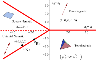
Figure 1: The phase diagram for a spin-two spinor condensate. The dashed line corresponds to the additional phase boundary dividing the nematic phase into two phases, a uniaxial nematic phase and a square nematic phase.

Fluctuations: We follow the standard Bogoliubov theory of the weakly interacting Bose gas to derive the spectrum of fluctuations. Consider decomposing the field operator into a dominant c-number piece, the mean field expectation value, and a smaller fluctuation piece $\psi(r)=\sqrt{n_{0}}\phi_{\eta}+\delta\Psi(r)$. Substituting this in the Hamiltonian we expand to quadratic order in the fluctuations (linear terms vanish on choosing the mean field solution) and diagonalize the resulting Bogoliubov Hamiltonian ${\cal H}_{B}$. This is aided by defining new canonical bosons via the linear combinations: $b_{1}\!=\!-\frac{i}{\sqrt{2}}(\delta\Psi_{1}+\delta\Psi_{-1})$, $b_{2}\!=\!-\frac{1}{\sqrt{2}}(\delta\Psi_{1}-\delta\Psi_{-1})$, $b_{3}\!=\!\frac{i}{\sqrt{2}}(\delta\Psi_{2}-\delta\Psi_{-2})$, and $f_{\pm}\!=\!\frac{1}{\sqrt{2}}\delta\Psi_{0}\pm\frac{i}{2}(\delta\Psi_{2}+\delta\Psi_{-2})$. Further, we define $p=\frac{1}{\sqrt{2}}(e^{i\eta}f_{+}+e^{i\eta}f_{-})$ and $q=\frac{1}{\sqrt{2}}(-ie^{i\eta}f_{+}+ie^{i\eta}f_{-})$. The Bogoliubov Hamiltonian assumes a particularly simple form in these variables. Defining velocities $v_{j}$ via $mv^{2}_{j}=[(2\beta-\gamma)n_{0}-2\beta n_{0}\cos(2\eta+\frac{2\pi j}{3})]$, or equivalently

$$v_{j}^{2}=\frac{4\pi n_{0}\hbar^{2}}{5m^{2}}\left[-(a_{0}-a_{4})+\frac{10}{7}(a_{2}-a_{4})\cos(2\eta+\frac{4\pi}{3}j)\right].$$ (2)

Then we have

$${\cal H}_{B} = \sum_{{\bf k}}\sum_{j=1}^{3}[mv^{2}_{j}+\frac{\hbar^{2}{\bf k}^{2}}{2m}]b^{\dagger}_{j{\bf k}}b_{j{\bf k}}-\frac{1}{2}mv^{2}_{j}(b^{\dagger}_{j{\bf k}}b^{\dagger}_{j{\bf-k}}+b_{j{\bf k}}b_{j{\bf-k}})$$ (3)

$$+ [(\alpha+\gamma)n_{0}+\frac{\hbar^{2}{\bf k}^{2}}{2m}]p^{\dagger}_{{\bf k}}p_{{\bf k}}+\frac{(\alpha+\gamma)n_{0}}{2}(p^{\dagger}_{{\bf k}}p^{\dagger}_{{\bf-k}}+p_{{\bf k}}p_{{\bf-k}})$$

$$+ [-\gamma n_{0}+\frac{\hbar^{2}{\bf k}^{2}}{2m}]q^{\dagger}_{{\bf k}}q_{{\bf k}}+\frac{\gamma n_{0}}{2}(q^{\dagger}_{{\bf k}}q^{\dagger}_{{\bf-k}}+q_{{\bf k}}q_{{\bf-k}}).$$

We see that these modes are completely decoupled and readily diagonalized by the Bogoliubov transformation. Physically, the $b_{j}$ modes are connected to spin rotations about the three coordinate axes with the spectrum $\omega_{j}(k)=k\sqrt{v^{2}_{j}+\hbar^{2}k^{2}/4m^{2}}$ ($j=1,\,2,\,3$). The $p$ boson generates phase fluctuations of the condensate and hence has the spectrum $\omega_{4}(k)=k\sqrt{(\alpha+\gamma)n_{0}/m+\hbar^{2}k^{2}/4m^{2}}$ which involves the compressibility $n_{0}(\alpha+\gamma)$. Finally the $q$ mode corresponds to fluctuations of the $\eta$ parameter and has the spectrum $\omega_{5}(k)=k\sqrt{(-\gamma)n_{0}/m+\hbar^{2}k^{2}/4m^{2}}$. Note, in the long wavelength limit all these modes have a linear dispersion. However, for a generic nematic superfluid, only the first four are goldstone modes of the broken spin and phase symmetry; the fifth will actually acquire a gap once the degeneracy between the different $\eta$ configurations is removed. The contribution of these modes to the free energy is readily calculated. However, only the dispersion of the $b_{i}$ modes depends on the nematic parameter $\eta$ and will be responsible for lifting the accidental degeneracy. The contribution from these modes $\frac{\Delta F(\eta)}{V}=T\sum_{n=1}^{3}\int{\frac{d^{3}\mathbf{k}}{(2\pi)^{3}}\log(2\sinh\frac{\hbar\omega_{n}(k)}{2T}})$ where $V$ is the volume, will be discussed below.

Order by Disorder:

Figure 2: Evolution of the free energy difference between uniaxial and square biaxial nematic states as a function of temperature with ⁸⁷Rb parameters.

Before evaluating the free energy, we make some general observations arising from symmetry. For this purpose the nematic region of the phase diagram is best described in terms of the variables $(a_{0}-a_{4})$, the $x$-axis in Fig. 1, and the ratio $\sigma=\frac{10}{7}\frac{a_{4}-a_{2}}{a_{0}-a_{4}}$. The nematic region corresponds to $(a_{0}-a_{4})<0$ and $|\sigma|<1$. Inspecting the velocities Eq. (2) one sees that the degeneracy remains unresolved along the line $\sigma=0$, which is also the phase boundary for the full Hamiltonian due to the enlarged symmetry. The symmetry breaking grows on moving away from this axis, but has opposite effects on either side of this line. Formally, the transformation $\sigma\rightarrow-\sigma,\,\eta\rightarrow\eta+\pi/2$ leaves the approximate free energy invariant.

At zero temperature, the free energy reduces to the contribution to the ground state energy for different nematic states from the zero point motion of the harmonic modes. Remarkably, this energy splitting $\Delta E(\eta)$ may be evaluated in closed form up to an overall constant :

$$\frac{\Delta E(\eta)}{V} = \frac{8m^{4}}{15\pi^{2}\hbar^{3}}\sum_{j=1}^{3}v_{j}^{5}$$ (4)

$$= \frac{8\hbar^{2}}{15\pi^{2}m}\left[\frac{4\pi n_{0}(a_{4}-a_{0})}{5}\right]^{\frac{5}{2}}g_{\frac{5}{2}}(\eta,\,\sigma)$$

where it is convenient to define the series of functions: $g_{m}(\eta,\,\sigma)=\sum_{j=1}^{3}[1+\sigma\cos(2\eta+\frac{2\pi j}{3})]^{m}$. The ground state is the one with the lowest combination of velocities, and turns out to be the square biaxial nematic state ($\eta=\pi/2$) for $\sigma>0$, and the uniaxial state for $\sigma<0$ ($\eta=0$). The latter is relevant to the experimental systems spin-2 ⁸⁷Rb and ²³Na, which both are believed to have $\sigma\approx-1$ .

At finite temperatures, thermal fluctuations are much more effective at lifting this degeneracy; again the state with the smaller combination of velocities and hence a larger population of thermal excitations will be entropically favored. While this may be evaluated numerically, there is a broad range of temperatures $T_{c}\gg T\gg{\rm max}(mv_{i}^{2})$ where it greatly simplifies. The lower limit is a rather small scale, related to the magnetic energy and about $1$nK for ⁸⁷Rb in Schmaljohann et al. (2004). In this limit, the linearly dispersing modes obey the equipartition law, and the leading term in the free energy that lifts the degeneracy is :

$$\frac{\Delta F(\eta)}{V} = -\frac{2}{3\pi}k_{B}T\sum_{j}(\frac{mv_{j}}{\hbar})^{3}$$ (5)

$$= -\frac{2}{3\pi}k_{B}T\left[\frac{4\pi n_{0}(a_{4}-a_{0})}{5}\right]^{\frac{3}{2}}g_{\frac{3}{2}}(\eta,\sigma)$$

On evaluating this expression, thermal fluctuations are found to lead to the same ground states as quantum fluctuations. A plot of the free energy variation with $\eta$ for $\sigma\approx-1$ is in the top curve of figure 3.

At higher temperatures the depletion of the condensate becomes important. This may be readily taken into account by using the temperature dependent condensate density obtained from mean field theory, which for a harmonic trap is $n(T)=n_{0}[1-(T/T_{c})^{3}]$. This temperature dependence has a significant effect only near $T_{c}$ and leads to a vanishing of the above free-energy splitting on approaching $T_{c}$, assuming a continuous transition. This temperature dependence of the free energy splitting between uniaxial and square biaxial states is shown in Fig. 2. for the parameters of ⁸⁷Rb in Schmaljohann et al. (2004).

These results may be caricatured by an effective Landau theory, where sixth order terms are generated by fluctuations. While a full discussion of all such terms is undertaken elsewhere Turner et al. , we note here that writing the five component order parameter as a symmetric traceless matrix $\chi$ Mermin (1974), allows for a 6th order term $\frac{32A}{3}\rm{tr}[\chi^{3}\chi^{*3}]$ in the free energy. This term, when evaluated in the nematic subspace yields $A|\chi_{0}|^{6}\cos 6\eta$, where $\chi_{0}$ is the magnitude of the order parameter. Clearly, if $A>0$, then the free energy is minimized by the square biaxial state $\eta=\pi/2,\,\pi/6,\,5\pi/6$, while if $A<0$, then the free energy is minimized by the uniaxial state $\eta=0,\,\pi/3,\,2\pi/3$. This sixth order term vanishes rapidly on approaching the transition, accounting for the near degeneracy of nematic ordered states near this point. Finally, it may be recalled that biaxial nematics are rather difficult to obtain in liquid crystal systems. Within Landau theory this is explained by the presence of a cubic term in the free energy $B{\mbox{tr~{}}}[\chi_{R}^{3}]$ when the nematic order parameter is a real symmetric traceless matrix. This can be shown to favor the uniaxial state regardless of the sign of $B$. However, in the spinor condensate, the fact that the spin 2 field also carries a charge quantum number implies the absence of such a term (it is a complex symmetric matrix with phase symmetry). Hence biaxial nematics may be realized, and would naturally occur in the $\sigma>0$ part of the nematic phase region. In addition to the topological defects with non-abelian homotopy for the general biaxial nematic, the square biaxial nematic realized here also has half superfluid vortices bound to a spin defect.

Experimental Prospects: Magnetic fields make the phase diagram more complex because the splitting due to fluctuations receives competition from the quadratic Zeeman energy $H_{qz}=-cB^{2}\int d^{3}\mathbf{x}{\psi^{\dagger}F_{z}^{2}\psi}$ , which favors the square uniaxial state. For weak fields the nematic axis drops into the $xy$ plane $\eta=\pi/3,\,2\pi/3$ because ${\,|\,F_{x}=0\,\rangle\,}=(\sqrt{\frac{3}{8}},0,\frac{1}{2},0,\sqrt{\frac{3}{8}})$ has lower $H_{qz}$ than ${\,|\,F_{z}=0\,\rangle\,}$. On increasing the field, the state continuously approaches the square state $\eta=\pi/2$. In Schmaljohann et al. (2004) a 50-50 split between atoms with $F_{z}=\pm 2$ was observed consistent with a square state; we believe this to be due to the relatively large background field reported in the experiments that overcomes the order by disorder effect. To observe the latter effect, a lower magnetic field as estimated below is needed. A possible way to observe the uniaxial to square state transition is by measuring the fraction of atoms with $F_{z}=0$ along a quantization axis parallel to the magnetic field as it drops from 25% for uniaxial states to zero for the square state (See Fig. 4). Magnitudes of fluctuation induced free energy splittings are shown in Table 1 for ⁸⁷Rb and ²³Na both at zero temperature and at $100$nK (roughly half the critical temperature for the density in Schmaljohann et al. (2004)). The critical field beyond which the quadratic Zeeman effect dominates is shown in the last column. Given that magnetic fields as low as $50\mathrm{mG}$ are readily accessible in current experiments Sadler et al. (2006), we believe these effects are within experimental reach. The effect could also possibly be used to access the condensate temperature by measuring the critical field. In a trap, an important consideration is that the linear part of the spin wave dispersions must be above the quantization scale of the trap, $\hbar\omega_{\mathrm{trap}}<m\;\mathrm{max}(v_{i}^{2})$.

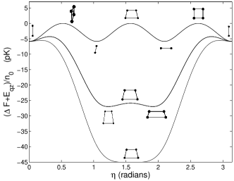
Figure 3: Evolution of the uniaxial nematic into square biaxial-nematic in a field. The free-energy, with a constant subtracted, is plotted in $pK$ per atom for the conditions of Ref Schmaljohann et al. (2004), for $B=0,20,27$mG (top to bottom). Reciprocal spinors are also shown. At the minima, they deform continuously from rectangles into squares as the field is increased. The Ising-like symmetry breaking at the critical field corresponds to making a choice between which way to deform the square.

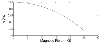
Figure 4: Proportion of $F_{z}=0$ component as magnetic field is increased to the critical field, for rubidium at density $4\times 10^{14}\mathrm{cc}^{-1}$ and $T=100\mathrm{nK}$.

	$\Delta E$	$\Delta F$	$B_{c}$
87Rb	$0.3$ pK	$6$ pK	$27$ mG
23Na	$3$ pK	$9$ pK	$19$ mG

Table 1: Free energy splittings at $T=0$, $T=100$nK, and critical fields, calculated for $n=4\times 10^{14}\mathrm{cc}^{-1}$ - the experimental conditions in Ref. Schmaljohann et al. (2004). Sodium has a greater disparity in its scattering lengths but has a stronger quadratic Zeeman effect, explaining its lower critical field.

In conclusion, the role of fluctuations in selecting the ground state spin structure of a spin-2 nematic condensate were studied. Both quantum and thermal fluctuations were shown to lead to the phase diagram in Fig. 1. For the experimentally interesting cases of ²³Na and ⁸⁷Rb, these effects compete against the quadratic Zeeman term, but can predominate for sufficiently weak fields. An Ising transition marks this point, which we believe can be accessed readily in future experiments. If so, this would be one of the first experimental demonstrations of the ‘order-by-disorder’ effect widely studied in the context of frustrated quantum magnetism.

We would like to thank Daniel Podolsky, Gil Refael and Dan Stamper-Kurn for insightful discussions and Fei Zhou for alerting us to Song et al. , where similar results are obtained. Support from from the Hellman Family Fund and LBNL DOE-504108 (A.V.), NSF Career Award, AFOSR and Harvard-MIT CUA (E.D. and A.M.T.) and the Sherman Fairchild Foundation (R.B.) are acknowledged.

References

- Stenger et al. (1998) J. Stenger, S. Inouye, D. M. Stamper-Kurn, H. J. Miesner, A. P. Chikkatur, and W. Ketterle, Nature 396, 345 (1998).
- Schmaljohann et al. (2004) H. Schmaljohann, M. Erhard, J. Kronjäger, M. Kottke, S. van Staa, L. Cacciapuoti, J. J. Arlt, K. Bongs, and K. Sengstock, Phys. Rev. Lett. 92, 040402 (2004).
- Chang et al. (2004) M. S. Chang, C. D. Hamley, M. D. Barrett, J. A. Sauer, K. M. Fortier, W. Zhang, L. You, and M. S. Chapman, Phys. Rev. Lett. 92, 140403 (2004).
- Griesmaier et al. (2005) A. Griesmaier, J. Werner, S. Hensler, J. Stuhler, and T. Pfau, Phys. Rev. Lett. 94, 160401 (2005).
- Sadler et al. (2006) L. E. Sadler, J. M. Higbie, S. R. Leslie, M. Vengalattore, and D. M. Stamper-Kurn, Nature 443, 312 (2006).
- Ho (1998) T. L. Ho, Phys. Rev. Lett. 81, 742 (1998).
- Ohmi and Machida (1998) T. Ohmi and K. Machida, J. Phys. Soc. Japan 67, 1822 (1998).
- Ciobanu et al. (2000) C. V. Ciobanu, S. K. Yip, and T. L. Ho, Phys. Rev. A 61, 033607 (2000).
- Zhou (2001) F. Zhou, Phys. Rev. Lett. 87, 080401 (2001).
- Barnett et al. (2006) R. Barnett, A. Turner, and E. Demler, Phys. Rev. Lett. 97, 180412 (2006).
- Casimir (1948) H. Casimir, , Proc. Kon. Nederland. Akad. Wetensch. B 51, 793 (1948).
- Villain (1979) J. Villain, Z. Phys. B. 33, 31 (1979).
- Henley (1989) C. L. Henley, Phys. Rev. Lett. 62, 2056 (1989).
- (14) A. Turner, R. Barnett, E. Demler, and A. Vishwanath, in preparation.
- Mermin (1974) N. D. Mermin, Phys. Rev. A 9, 868 (1974).
- (16) J. L. Song, G. Semenoff, and F. Zhou, cond-mat/0702052.