Transport of interface states in the Heisenberg chain

Abstract

We demonstrate the transport of interface states in the one-dimensional ferromagnetic Heisenberg model by a time dependent magnetic field. Our analysis is based on the standard Adiabatic Theorem. This is supplemented by a numerical analysis via the recently developed time dependent DMRG method, where we calculate the adiabatic constant as a function of the strength of the magnetic field and the anisotropy of the interaction.

, ,

1 Introduction

The problem of calculating the dynamics of quantum spin chains has acquired new importance due to potential new applications in spintronics [1, 2], quantum information, computation and control theory and the now realistic possibility of doing experiments on systems that are accurately described by a one-dimensional array of spins [3, 4]. The development of time-dependent versions of the successful Density Matrix Renormalization Group (DMRG) method of White [5, 6] by several authors [7, 8, 9, 10] therefore comes at a fortuitous moment. All numerical schemes for a quantum many-body problem such as a spin chain necessarily involve a drastic reduction of the high-dimensional Hilbert space to a suitable subspace of relatively modest dimension. The DMRG method does this by approximating the desired states (typically the ground state and low-lying excitations above it) by finitely correlated states [11], also known as generalized valence bond states or matrix product states. The time-dependent DMRG method extends this idea by allowing the subspace used in the approximation scheme to depend on time.

Here we are interested in the dynamics of the Heisenberg XXZ chain with kink boundary conditions [12] and a time-dependent external field. The ground states of this model are the so-called kink states which describe an interface between domains of opposite magnetization. Their degeneracy grows with the length of the chain [13, 14], and is labelled by the position of the kink, or equivalently, the total magnetization which is a conserved quantity. A transverse external field localized at one site can be used to select a unique ground state [15], i.e., such a perturbation pins the kink at a specific site. These interface structures also appear in certain asymmetric simple exclusion models of stochastic particle dynamics [16, 17, 18] and it is a natural question to study their non-equilibrium properties. In this paper we study the quantum dynamics of the kink under the influence of a time-dependent magnetic field. Typically we use a field supported at one or two sites and moving at a constant speed. For small velocities, we know by the adiabatic theorem that the time-evolution of a ground state will follow the ground state of the time-dependent Hamiltonian. The standard heuristic scale to identify the adiabatic regime is the smallness of the ratio of the time-derivative of the Hamiltonian over the spectral gap squared. We will verify the usefulness of this criterion by calculating the time evolution of kink states in the XXZ chain under the influence of a time-dependent magnetic field. Needless to say, the dynamics of kink states, which can be regarded as discrete analogues of solitons, is of great interest in its own right. Moreover, they provide a simple dynamical quantum model of sharp magnetic domain walls.

In order to numerically study the quality of the adiabatic approximation and its domain of validity, it is necessary to express the evolved state in the time-dependent eigenbasis of the Hamiltonian. Therefore we construct the DMRG basis at time $t$ starting from the ground state(s) and low-lying excited states of the Hamiltonian of the system at time $t$. This is in contrast with the original method, where the time-dependent DMRG basis is obtained from the evolved state at time $t$. Our method can be of more general interest, since the calculation of the DMRG basis is a separate calculation about which we can be confident to have good control, regardless of the potential difficulties in reliably calculating the time evolution.

The paper is organized as follows. In Section 2, we define the model and study its basic properties. The adiabatic approximation is studied in Section 3. In Section 4, we give a brief discussion of the issues that arise with rapidly changing magnetic fields. Details of the DMRG algorithm are given in A.

2 The model

The spin-$\frac{1}{2}$ ferromagnetic XXZ Heisenberg model on the chain $[1,L]$ with interface boundary conditions is defined by the Hamiltonian $H_{0}=\sum_{x=1}^{L-1}h_{x,x+1}$, with nearest-neighbor interaction

$$h_{x,x+1}=-\Delta^{-1}(S_{x}^{1}S_{x+1}^{1}+S_{x}^{2}S_{x+1}^{2})-S_{x}^{3}S_{x+1}^{3}+{\textstyle\frac{1}{2}}\sqrt{1-\Delta^{-2}}(S_{x}^{3}-S_{x+1}^{3})+{\textstyle\frac{1}{4}}\Eins\,,$$ (1)

where $\Delta>1$ is the anisotropy parameter and the matrices $(S_{x}^{1},S_{x}^{2},S_{x}^{3})$ are the usual spin-$\frac{1}{2}$ matrices; $h_{x,x+1}$ is a projection and $H_{0}$ has ground state energy zero. We have set $\hbar=1$ which should be kept in mind when we define adiabatic regimes in terms of the magnitude of the magnetic field and the velocity.

The Hamiltonian $H_{0}$ acts on the Hilbert space ${\mathcal{H}}_{L}=\mathbb{C}^{2^{L}}$. It has a large (quantum) symmetry with a similar multiplet structure as the $SU(2)$-symmetric, isotropic model where $\Delta=1$. In the limit $\Delta\to\infty$ we obtain the Ising Model, $H^{\mathrm{Ising}}=H_{0}(\Delta=\infty)$. The ground states and excited states (for finite $L$ and in the infinite volume limit $L\to\infty$) have been analyzed completely in recent years [19, 20, 21, 22, 23]. A convenient basis of ground states are the so-called grand canonical ground states, $\phi_{c}$. They are product states and depend on a complex parameter $c\in\mathbb{C}\setminus\{0\}$:

$$\phi_{c}=\bigotimes_{x=1}^{L}\left[(1+|c|^{2}q^{2x})^{-1/2}\left(\begin{array}[]{c}1\\ cq^{x}\end{array}\right)\right]\,.$$ (2)

The state $\phi_{c}$ describes an interface state that is exponentially localized at $x_{0}=-\ln{|c|}/\ln{q}$ with $q=\Delta-\sqrt{\Delta^{2}-1}\in(0,1)$. The width of the interface depends on $\Delta$ and becomes sharp (i.e., the transition from up to down spin occurs across one bond) in the Ising limit $\Delta\to\infty$ and flat as $\Delta\downarrow 1$. There are no interface states in the isotropic Heisenberg model.

We perturb the Hamiltonian by a magnetic field ${\mathbf{B}}:[1,L]\rightarrow\mathbb{R}^{3}$ satisfying the locality condition:

(A1)

The support of ${\mathbf{B}}$ is finite, non-empty, and independent of $L$.

Then we define the Hamiltonian

$$H_{V}=H_{0}+V\quad\mathrm{with}\quad V=\sum_{x}{\mathbf{B}}(x)\cdot{\mathbf{S}}_{x}\,.$$ (3)

We refrain from considering the infinite chain limit in detail. Condition (A1) ensures that $H_{V}$ is still a well-defined semi-bounded operator in the GNS representation of the unperturbed Hamiltonian.

The case of a magnetic field located at a single site $y$ has been analyzed in [15]. Let $B_{1}+\mathrm{i}B_{2}\not=0,c_{y}=-(\|{\mathbf{B}}\|+B_{3})(B_{1}+\mathrm{i}B_{2})^{-1}q^{-y}$, and let $\phi_{c_{y}}$ be a state of the form (2). This state $\phi_{c_{y}}$ has energy $-\frac{1}{2}\|{\mathbf{B}}\|$, and since the ground state energy can be at most shifted by this amount, we know that it is a ground state. It is also the unique ground state which moreover has a uniform gap as $L\to\infty$. If $\mathbf{B}=(B,0,0)$ with $B\not=0$, then $\phi_{c_{y}}$ is a kink localized at site $y$. If ${\mathbf{B}}(x)=(0,0,B(x))$ with $B(x)\leq 0$, then the ground state is the all spin-up state which, as $L\to\infty$ is however not in the GNS kink Hilbert space; see the discussion in [15].

In the Ising limit $\Delta\to\infty$, ground states may be largely degenerate as for $V=0$. For example, consider the magnetic field ${\mathbf{B}}(1)=(1,0,0),{\mathbf{B}}(2)=(0,0,1)$, and zero otherwise. Then $H_{V}$ has $L-1$ “kink” ground states of the form $\psi_{[1,2]}\otimes\psi_{[3,L]}$. Here, $\psi_{[1,2]}$ is the ground state of the two-site Hamiltonian which has the form $\psi_{[1,2]}=(0,c,0,-\sqrt{1-c^{2}})$ for some $c>0$. Note that $\langle\psi_{[1,2]}|S_{2}^{3}\psi_{[1,2]}\rangle=-1/2$. Thus we can choose $\psi_{[3,L]}$ to be an (Ising) kink state on the remaining sites of which there are $L-1$.

Thus we consider fields ${\mathbf{B}}$ such that for all $x$ with ${\mathbf{B}}(x)\not=0$, ${\mathbf{B}}(x)$ has a non-vanishing component in the $xy$-plane. This means that, in addition to (A1), we assume the following:

(A2)

On the support of $V$, ${\mathbf{B}}(x)\not=(0,0,\pm\|{\mathbf{B}}(x)\|)$.

Theorem 2.1.

Let ${\mathbf{B}}$ satisfy the conditions (A1) and (A2). Then, there exists a finite $\Delta_{0}=\Delta_{0}({\mathbf{B}})$ so that for all $\Delta>\Delta_{0}$,

1. $H_{V}$ defined in (3) has a unique ground state;

2. $H_{V}$ has a positive gap above the ground state uniformly in $L$. I.e., there exists a $\gamma(\Delta)>0$, independent of $L$, such that for all states $\psi$ orthogonal to the ground state we have $\langle\psi|(H_{V}-E_{0})|\psi\rangle\geq\gamma\,\|\psi\|^{2}$.

The conclusions of the theorem can be expected to be valid for other situations than the ones covered by (A1) and (A2). In the cases where we have performed numerical calculations, a positive gap appeared for all $\Delta>1$. Here we only show the result for sufficiently large $\Delta$ by applying the theory of relatively bounded perturbations, see e.g. [24]. Let us recall that an operator $B$ is relatively bounded with respect to the operator $A$ if there exists a (finite) constant $M$ so that for all $\psi$ in the domain of $A$, $\|B\psi\|\leq M\big{(}\|A\psi\|+\|\psi\|\big{)}$. Then, all eigenvalues and eigenprojections in the discrete spectrum (i.e., isolated and finite multiplicity) of $A(\alpha)=A+\alpha B$ are analytic for $\alpha\in(-\alpha_{0},\alpha_{0})$ for some $\alpha_{0}>0$ (cf. [24, 3.5.14]).

Proof.

Let $H_{V}^{\mathrm{Ising}}=H_{V}(\Delta=\infty)$ be the Ising kink Hamiltonian with magnetic field ${\mathbf{B}}$. By using a rotation around the $z$-axis we can assume that ${\mathbf{B}}(x)=(B^{1}(x),0,B^{3}(x))$ with $B^{1}(x)<0$ for all $x$ in the support $[a,b]$ of ${\mathbf{B}}$. Then the Hamiltonian $H_{V,[a,b]}^{\mathrm{Ising}}$ defined on the support of ${\mathbf{B}}$ has a unique ground state $\psi_{[a,b]}$ by the usual Perron-Frobenius argument. I.e., there is an $n\in\mathbb{N}$ such that $\big{(}H_{V,[a,b]}^{\mathrm{Ising}}\big{)}^{n}$ has strictly negative off-diagonal entries. We claim now that $\psi_{[1,L]}=\bigotimes_{x=1}^{a-1}{0\choose 1}\otimes\psi_{[a,b]}\otimes\bigotimes_{x=b+1}^{L}{1\choose 0}$ is the ground state of $H_{V}^{\mathrm{Ising}}$ on the full chain $[1,L]$. By adding the other (non-negative) Ising Hamiltonians to the left and right of the support of ${\mathbf{B}}$ the ground state energy could in principle increase. But $\psi_{[1,L]}$ is also an eigenvector of $H_{V}^{\mathrm{Ising}}$ with the same eigenvalue as $\psi_{[a,b]}$ since the additional terms vanish on $\psi_{[1,L]}$. Thus $\psi_{[1,L]}$ is the ground state of $H_{V}^{\mathrm{Ising}}$.

Next, we consider the Heisenberg Hamiltonian $H_{V}(\Delta)=H_{V}^{\mathrm{Ising}}+\Delta^{-1}K+(1-\sqrt{1-\Delta^{-2}})P$. $P$ only involves the boundary spins and is therefore uniformly bounded. $K$ contains the $XY$ terms in the Hamiltonian and the norm of this term is of order $L$. In particular, it is not uniformly bounded but one can show that $K$ is relatively bounded with respect to $H_{V}^{\mathrm{Ising}}$. This was done in [25] for the Hamiltonian without $B$-field. The relative bound is uniform in $L$. By our assumptions, the $B$-field defines a bounded operator and hence $K$ is also relatively bounded with respect to $H_{V}^{\mathrm{Ising}}$. It follows that for $\Delta^{-1}$ in a non-empty interval $[0,\Delta_{0}^{-1}]$, the spectral projection for an interval of energies containing the unperturbed ground state energy is an analytic function of $\Delta^{-1}$. This implies the statement of the theorem. ∎

Our prime example are magnetic fields located on two adjacent sites, $x_{0}=L/2$ and $x_{0}+1$. More precisely, let $v,\,B>0$ and define

$$B(x,t) =-B\cdot f(x-vt)\,,$$

$$f(x) =\cases{1-|x-x_{0}|&for $x_{0}-1\leq x\leq x_{0}+1$\\ 0&otherwise\\ }\,.$$

The perturbation

$$V(t)=\sum_{x=1}^{L}B(x,t)S_{x}^{1}=-(1-vt)\,B\,S_{x_{0}}^{1}-vt\,B\,S_{x_{0}+1}^{1}$$ (4)

for $0\leq t\leq\tau=1/v$ satisfies the conditions (A1) and (A2). Hence, we know from Theorem 2.1 that the Hamiltonian,

$$H(t)=H_{0}+V(t)$$ (5)

has a unique ground state, $\varphi(t)$, with a positive gap. The ground state energy $E_{0}(t,B)$ is analytic on $(0,v^{-1})$, also as $L\to\infty$. It is well-known [24, 3.5.23] that the ground state energy $E_{0}(t,B)$ is concave in $t$. By symmetry we also have $E_{0}(t,B)=E_{0}(v^{-1}-t,B)$ for $0\leq t\leq 1/(2v)$. This implies $E_{0}(1/2v,B)=\max_{t}E_{0}(t,B)$. We can get more information on $E_{0}(t,B)$ from the low energy spectrum of the Hamiltonian with the magnetic field at a single site. For simplicity we put $v=1$.

Proposition 2.2.

For $t>0$ let $g(t)$ be the gap above the ground state $\phi_{c_{y}}$ of $H_{y}(t)=H_{0}-tBS_{y}^{1}$. Then $g(t)$ is increasing in $t$ (strictly speaking, $g(t)$ also depends on $L$ which we will tacitly ignore). Further, on $[0,1/2]$ we have for the Hamiltonian $H(t)$ defined through (4) and (5),

$$H(t)\geq\frac{1}{2}\,g(2t)\,\big{(}1-|\langle\phi_{c_{y}}|\phi_{c_{y+1}}\rangle|\big{)}\,.$$

Proof.

We may assume that $B>0$; otherwise apply a rotation. That $g(t)$ is increasing follows from the variational principle. To this end, let $0<t<t^{\prime}$. Let $\psi$ be orthonormal to $\phi_{c_{y}}$ such that $\left\langle\psi\right|H_{y}(t^{\prime})+\frac{1}{2}t^{\prime}B\left|\psi\right\rangle=g(t^{\prime})$. Then,

$$\left\langle\psi\right|H_{y}(t)+\frac{1}{2}tB\left|\psi\right\rangle\\ =g(t^{\prime})+(t-t^{\prime})B\left\langle\psi\right|\frac{1}{2}-S_{y}^{1}\left|\psi\right\rangle\,\leq\,g(t^{\prime})\,.$$

Thus, $g(t)\leq g(t^{\prime})$. The estimate on the ground state energy of $H(t)$ is based on Kitaev’s Lemma [26, Lemma 14.4]. In general, let $A_{1}$ and $A_{2}$ be two operators on some Hilbert space $\mathcal{H}$. By $G_{1,2}$ and $\Pi_{1,2}$ we denote the space of ground states and the orthogonal projections onto $G_{1,2}$, respectively. We assume that $G_{1}\cap G_{2}=\{0\}$, and that for some $\delta>0$, $A_{1,2}\geq\delta(1-\Pi_{1,2})$. Then,

$$A_{1}+A_{2}\geq\delta\Big{(}1-\sup_{\psi_{1,2}\in G_{1,2}}\big{|}\langle\psi_{1}|\psi_{2}\rangle\big{|}\Big{)}\,.$$

For our proof it suffices to apply this inequality with

$$A_{1} ={\textstyle\frac{1}{2}}H_{0}-(1-t)B(S_{y}^{1}-{\textstyle\frac{1}{2}}\Eins)={\textstyle\frac{1}{2}}H_{y}(2(1-t))+{\textstyle\frac{1}{2}}(1-t)B\Eins\geq 0\,,$$

$$A_{2} ={\textstyle\frac{1}{2}}H_{0}-tB(S_{y+1}^{1}-{\textstyle\frac{1}{2}}\Eins)={\textstyle\frac{1}{2}}H_{y+1}(2t)+{\textstyle\frac{1}{2}}{tB}\Eins\geq 0\,.$$

∎

We supplement this analysis of the ground state properties of the family of Hamiltonians (5) with numerical DMRG calculations for a chain of length $L=20$ and an anisotropy of $\Delta=2$. The chain length is chosen such that for given $\Delta$, $L$ is much larger than the width of the interface, but otherwise there are no qualitative differences for different combinations of $\Delta$ and $L$. We distinguish three ranges of $B$-values with qualitatively different ground state properties.

A typical intermediate value of $B$ is $0.5$. The $S^{3}$-magnetization profile of the ground states $\varphi(t)$ of $H(t)$ nicely interpolates between the interface product states $\varphi(0)=\phi_{c_{x_{0}}}$ and $\varphi(1)=\phi_{c_{x_{0}+1}}$ (see eq. (2)) with $x_{0}=L/2$ (Figure 1). The first excited states are still well localized around the interface positions. Both the ground state and first excited state energies are concave as a function of $t$ (Figure 2). The ground state energy is minimal and equal to the known value $-B/2$ at the start ($t=0$) and end ($t=\tau$) points. The gap is always strictly positive, but minimal at half period ($t=\tau/2$). The transition from $\varphi(0)$ to $\varphi(1)$ is not homogeneous, in the sense that the right or top half of the interface moves first and the left or lower half moves later. This effect becomes more pronounced as $B$ increases (compare Figure 1 left and right) and can be understood as follows. In the first phase after switching on a magnetic field at $x_{0}+1$, $S_{x_{0}+1}^{1}$ has the effect of rotating the up vector at $x_{0}+1$ into the $(1,3)$-plane. But here nothing happens at site $x_{0}$ because the initial state is an eigenstate of $S_{x_{0}}^{1}$. The same thing happens at the end of the cycle when the vector at $x_{0}+1$ is almost an eigenvector of $S^{1}_{x_{0}+1}$. Site $x_{0}$ is affected only after some time as the perturbation at $x_{0}+1$ is communicated to $x_{0}$ in second order.

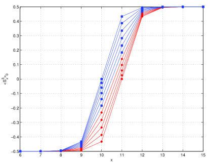
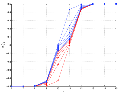
Figure 1: $S^{3}$-magnetization profiles of the ground states for $B=0.5$ (left) and $B=5$ (right), for $0\leq t\leq\tau/2$ (■) and $\tau/2\leq t\leq\tau$ (●) ($\tau=200$, $200$ time steps, profiles plotted for every $20$ time steps, only central sites around the interface are shown).

For very small magnetic fields, the ground state energy is still a concave function of $t$, but the first excited state energy is now convex (Figure 2). The energy gap is still minimal at half period. Furthermore the energy gap for a 10 times smaller magnetic field ($0.05$ vs. $0.5$) is approximately 10 times smaller, confirming the theoretical result [15] (for a single site impurity) that the gap scales linearly with $B$ for small $B$. For magnetic fields much larger than the intermediate value $B\approx 0.5$, the phenomenon that the interface moves in separate steps becomes much more pronounced (Figure 1). Like for intermediate $B$-values, the energies of the ground and first excited states are concave functions of $t$, but the minimal gap now occurs at the start and final times (Figure 2).

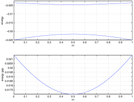
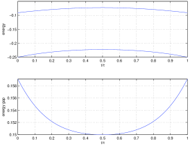
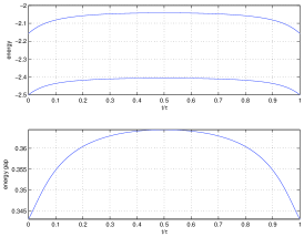
Figure 2: Energy of the ground states and first excited states (top) and energy gap (bottom) for $B=0.05$, $B=0.5$ and $B=5$ (left to right).

3 Adiabatic transport

Let us recall the standard adiabatic theorem which applies also to the case of an infinite chain. Let $\tau>0$ and $H(t)$, $0\leq t\leq\tau$, be a family of self-adjoint operators with common dense domain, and let $\psi(t)$ be the solution to

$$\mathrm{i}\frac{\partial}{\partial t}\psi(t)=\tau H(t)\psi(t)$$ (6)

with initial condition $\psi(0)$. By $P(t)$ we denote the spectral projection onto the ground states of $H(t)$. We assume that $P(t)$ is piece-wise, twice continuously differentiable, finite dimensional, and uniformly (in $t$) separated from the rest of the spectrum of $H(t)$ by a gap $\gamma(t)$.

Theorem 3.1 (Adiabatic Theorem, Kato).

Under the above conditions on $H(t)$ and $\psi(t)$, there is an eigenvector $\varphi(t)$ of $H(t)$ with $\varphi(0)=\psi(0)$ and a constant $C$ such that,

$$\sup_{0\leq t\leq\tau^{-1}}\|\psi(t)-\varphi(t)\|\leq C\tau^{-1}\,.$$ (7)

Proof.

See [27] or [24, 3.3.11]. ∎

We call the smallest constant $C$ in (7) the adiabatic constant. Heuristically [28, 17.112], the adiabatic constant is of the order

$$\sup_{s\in[0,1]}\frac{\|\frac{d}{ds}{H}(s)\|}{\gamma(s)^{2}}\,,\quad s=t/\tau\,.$$ (8)

In our case, $H(t)$ is given by (5), and $\|\frac{d}{ds}{H}(s)\|=\|BS_{x_{0}}^{1}-BS_{x_{0}+1}^{1}\|=B$. Hence, $C\propto B/\gamma_{\mathrm{min}}^{2}$ with $\gamma_{\mathrm{min}}=\min_{s\in[0,1]}\gamma(s)$ is the minimal gap. As $B$ tends to infinity the gap $\gamma$ saturates and therefore $C$ grows linearly with $B$ for large $B$. On the other hand, if $B$ is small then the gap shrinks like $B$ (not $B^{2}$) as has been shown for a single site perturbation [15], and $C$ diverges as $1/B$. As a consequence, there is an optimal range for which $C$ is smallest. In Figure 3 this appears near $B=1$. If we fix $B$ and $\Delta$ and some $\varepsilon$ we can find (empirically) an upper bound $v_{\max}$ for the velocity $v$ for which then the adiabatic evolution is $\varepsilon$-close (in the $\ell^{2}$-sense) to the true time evolution. The slowdown (decreased $v_{\max}$) of the domain wall motion for large $B$-fields was reported cf. [2]) but here we also observe a slowdown for small $B$-fields. On a rigorous level, estimates in the vein of (8) on the adiabatic constant were recently derived by Jansen, Ruskai, and Seiler [29].

We have computed the adiabatic constant numerically using adaptive time-dependent DMRG [7, 9]. Unlike the original method, we express the evolved state in the time-dependent eigenbasis of the Hamiltonian such that we can compute eq. (7) with $\psi(t)$ and $\varphi(t)$ expressed in the same basis (see A for algorithm details). Figure 3 shows the adiabatic constant as well as the heuristic upper bound

$$C\leq\alpha\frac{B}{\min_{s\in[0,1]}\gamma(s)^{2}}\,,$$

with the energy gaps computed by ground state DMRG (see Section 2). To determine $\alpha$, we took one value of $B$ ($B=1.0$ for $\Delta=2$ and $B=2.0$ for $\Delta=10$) and made the inequality in (8) an equality at the lowest $v$ ($v=0.001$) at this particular value of $B$.

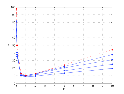
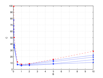
Figure 3: Adiabatic constant as a function of magnetic field strength $B$ for different velocities $v=0.01,0.005,0.002,0.001$ (——, bottom to top) compared to the upper bound $\alpha B/\gamma_{\rm min}^{2}$ (– – –) for anisotropy $\Delta=2$ (left, $\alpha=0.5677$) and $\Delta=10$ (right, $\alpha=0.6324$) with $L=20$.

Since our time-dependent algorithm does not target the state $\psi(t)$ directly, but rather the lowest energy states of the Hamiltonians $H(t)$ (see A), it is important to keep track of how well $\psi(t)$ is represented in these time-evolving DMRG bases. One way to measure this is by computing the deviation from $1$ of the norm of $\psi(t)$. As expected there is a correlation between this norm loss and the value of the adiabatic constant $C$. In Figure 3, where $C$ is minimal, $\|\psi(t)\|$ will be above $0.999$ at all times; at the very smallest and very largest $B$-fields, and for the largest velocities still considered adiabatic ($v\approx 0.01)$ the minimum norm drops to about $0.97$.

Adiabaticity is also measured by comparing the value of the total energy in the time-evolved state with the ground state energy of $H(t)$, i.e.,

$$\frac{\langle\psi(t)|H(t)|\psi(t)\rangle}{\|\psi(t)\|^{2}}-E_{0}(t)$$

should be close to $0$ at all times. For a typical adiabatic speed $v=0.005$ and intermediate $B$-field, this difference never exceeds $5\cdot 10^{-4}$. Energy differences in the small and large $B$ regions are of similar magnitude.

Finally, we comment on the role of the interpolation function (4) in our adiabatic Hamiltonian. Let us consider a large magnetic field. Then as time proceeds part of the profile is lagging behind (cfr. Figure 1). Also, the change of the profile is rather quick in the beginning (and at the end) and slow in the middle of a cycle. To improve on the transport of the domain wall for a fixed time interval we can take advantage of this phenomenon and slow down the time evolution in the beginning and accelerate in the middle by choosing a different interpolation function. In other words, we may use a general interpolating Hamiltonian $H_{f}(t)=H_{0}-(1-f(vt))BS_{x_{0}}^{1}-f(vt)BS_{x_{0}+1}^{1}$ with the constraint that $f(1)=1-f(0)=1$ to keep the same mean velocity. As an example we have used the function $f_{1}(t)=\cos(\pi t/2)$ and a piece-wise linear function $f_{2}$ with slope $1/3$ for $t\in[0,1/6]\cup[5/6,1]$ and slope $4/3$ on the interval $[1/6,5/6]$. In the first case we took $L=20,\Delta=2,B=5,v=0.05$ and reduced the adiabatic constant from 16.6 (constant velocity, or equivalently linear $f$) to 4.5 calculated with $f_{1}$. In the second example with $f_{2}$ and parameter values $L=20,\Delta=2,B=10,v=0.05$ the adiabatic constant dropped from 25.1 to 12.2. This observation is in agreement with [29], where the adiabatic constant for the general interpolating Hamiltonian $H_{f}(t)$ was studied.

4 Fast change of the magnetic field

Now we study the situation when the velocity of the moving magnetic field is large. We start initially in the ground state $\phi=\phi_{c_{x_{0}}}$ of the Hamiltonian $H(0)=H_{0}-BS_{x_{0}}^{1}$. Let $\tau=1/v$ and let $p(\tau)$ be the probability that at time $\tau$ the system is still in the state $\phi$. Then according to formula [28, (17.60)],

$$p(\tau)=1-\tau^{2}\,{\rm var}_{\phi}(\bar{H})+{\mathcal{O}}(\tau^{3})$$

with ${\rm var}_{\phi}(\bar{H})=\langle\phi|\bar{H}^{2}|\phi\rangle-\langle\phi|\bar{H}|\phi\rangle^{2}$, and $\bar{H}=\frac{1}{\tau}\int_{0}^{\tau}H(t)\,dt$. In our example, $\bar{H}=H_{0}-\frac{B}{2}(S_{x_{0}}^{1}+S_{x_{0}+1}^{1})$. Since $\phi$ is also an eigenstate of $H_{0}-\frac{B}{2}S_{x_{0}}^{1}$ with energy $-\frac{B}{4}$, we obtain

$$\langle\phi|\bar{H}|\phi\rangle=-\frac{B}{4}-\frac{B}{2}\langle\phi|S_{x_{0}+1}^{1}|\phi\rangle\,,\;\langle\phi|\bar{H}^{2}|\phi\rangle=\frac{B^{2}}{8}+\frac{B^{2}}{4}\langle\phi|S_{x_{0}+1}^{1}|\phi\rangle\,.$$

Hence,

$${\rm var}_{\phi}(\bar{H})=\frac{B^{2}}{16}\big{(}1-4\langle\phi|S_{x_{0}+1}^{1}|\phi\rangle^{2}\big{)}\,.$$

The quantity $\langle\phi|S_{x_{0}+1}^{1}|\phi\rangle$ can be computed fairly explicitly as a function of $\Delta$ but we are content with the trivial estimate that $1-4\langle\phi|S_{x_{0}+1}^{1}|\phi\rangle^{2}\leq 1$. As a result, the probability to stay in the initial state $\phi$ until $\tau$,

$$p(\tau)\geq 1-\frac{\tau^{2}B^{2}}{16}+{\mathcal{O}}(\tau^{3})\,.$$

If we want this to be larger than $1-\varepsilon$, then $|B|$ needs to be smaller than $4v\sqrt{\varepsilon}$.

Numerically we can also investigate the intermediate region between adiabatic and sudden change of the magnetic field. Here, $B$ and $v$ are of the same order of magnitude. In Figure 4, we follow the $S^{3}$-magnetization profile of the time evolved state over two periods, with the natural extension of $V(t)$ in (4) such that the field keeps moving to the right. Although the position of the interface is transported in the same direction as the magnetic field, it is lagging behind w.r.t. the postion of the ground state interfaces $\varphi(t)$ (which moves from site $10$ to site $12$). At the same time the width of the interface is growing bigger. Also the energy of $\psi(t)$ is lagging behind w.r.t. the periodicity of the spectrum of $H(t)$ (see Figure 4). The difference with the ground state energy is steadily increasing, and it is an interesting question whether this difference will eventually saturate. In this computation, the minimum norm of $\psi(t)$ remains above $0.99$ for the first period ($t\leq v^{-1}$) and above $0.97$ for the second period ($t\leq 2v^{-1}$)), so despite the non-adiabatic transport, $\psi(t)$ is still well represented in the DMRG basis constructed from the low-energy spectrum of $H(t)$. The overlap with the ground state $\varphi(t)$ drops to $0.80$ during the first period, and further to $0.71$ during the second period.

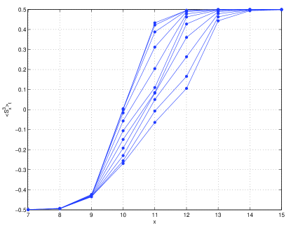
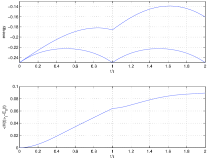
Figure 4: $S^{3}$-magnetization profiles of $\psi(t)$, for $0\leq t\leq\tau=2v^{-1}$ (left) and energy of the ground state and of $\psi(t)$ (right, top) and energy difference between $\psi(t)$ and the ground state (right, bottom) ($\Delta=2$, $B=0.5$, $v=0.1$, $200$ time steps, $S^{3}$-profiles plotted for every $20$ time steps).

We have tested other magnetic field perturbations such as a smooth field

$$V(t)=\frac{B}{4}\sum_{x}\bigl{(}1+\cos(\pi(x-vt))\bigr{)}^{2}\chi_{L}(x-vt)\,S^{1}_{x}$$

where

$$\chi_{L}(x)=\cases{1&for $x\in[L/2-1,L/2+1]$\\ 0&otherwise}$$

For $L$ a multiple of $4$, this is again a single-site perturbation for $t=nv^{-1}$, $n=0,1,2,\dots$, and interpolating smoothly in between. In this case, the non-differentiable curves in Figure 4 become smooth, but no other qualitative differences are observed.

Let us summarize the two regimes in terms of the two parameters $v$ and $B$. We are in the adiabatic regime if $Cv\ll 1$. Since for small $B$, the adiabatic constant $C$ is inverse proportional to $B$, we require $v\ll B$. For large $B$ we know that $C$ is proportional to $B$ and thus we want that $v\ll 1/B$. The regime where the initial state is stationary is simply given by the condition that $B\ll v$.

5 Summary

We have studied the propagation of a magnetic domain wall in the ferromagnetic Heisenberg chain due to a time dependent magnetic field. This situation is of immediate interest in submicrometer magnetic wires [2, 3] and in establishing ferromagnetic gates [1]. In the simplest case, the magnetic field is localized near the center of the domain wall (say at site $x_{0}$) and then moved along the chain to site $x_{1}$. If its velocity is small then we are in the adiabatic regime and the domain wall is shifted from $x_{0}$ to $x_{1}$ thereby preserving its shape. We find that there is an optimal region of the strength of $B$-fields for which the domain wall mobility is highest and is reduced for large and small $B$-fields.

On top of an analytical study using the standard Adiabatic Theorem and based upon properties of the Heisenberg model that have been proved in recent years, we have performed a numerical study. The latter is a variation of the recently developed time-dependent Density Matrix Renormalization Group method. This allows us to follow the Schrödinger time evolution of the domain wall with high accuracy in the adiabatic as well as the non-adiabatic regime, and discuss in detail the dependence on the parameters of our model such as the strength and speed of the magnetic field and the coupling constant in the Heisenberg interaction.

Appendix A DMRG algorithms

The DMRG algorithms for ground state [5] as well as time-dependent [7, 8, 9, 10] computations are well known, see also [30] and [6]. However, degeneracy and non-translation invariance of the ground states of the (translation invariant) XXZ kink Hamiltonian require a few non-standard adaptations. To lift degeneracy, we restrict to a sector of fixed total $S^{3}$-magnetization. For a chain of even length, the ground state with total magnetization zero has an interface centered in between the two middle sites. This state can be grown in the usual way by successively inserting two sites in the middle and targeting the zero magnetization state at each step. For a kink state with non-zero magnetization, we grow the system initially in the zero magnetization sector. If eventually a total magnetization with interface close to the middle is needed, we perform the finite system convergence sweeps in the new sector, with the zero magnetization state as initial trial state. If an interface close to one of the edges is needed, we grow the system at the right moment by targeting a magnetization sector which increases or decreases with one each step (effectively inserting two up or two down spins in the middle, thus shifting the kink to the right or left). The DMRG enlarging process implicitly assumes a translation invariant Hamiltonian. However, if the breaking of translation invariance is due to a local perturbation as in our case (with external magnetic fields located on one or two sites), we can grow the system targeting the zero magnetization kink, and add the perturbation for the finite system convergence sweeps where translation invariance is no longer needed. The DMRG state thus obtained converges indeed very rapidly to the true ground state $\psi(0)$ of the perturbed Hamiltonian (5) at time $t=0$.

In the standard time-dependent DMRG, adaptation of the basis is done by computing and truncating new reduced density matrices for the evolved state $\psi(t)$. Here the situation is different because we need to compute both the time evolved state $\psi(t)$ and the true ground state $\varphi(t)$ of $H(t)$ (in the same DMRG basis, naturally). Therefore we use the ground state (or several low-lying states) of $H(t)$ to adapt the Hilbert spaces. The details of our algorithm are as follows. The time period $[0,\tau]$ is first divided in $n_{\tau}$ time steps of length $\delta=\tau/n_{\tau}$ by discretizing the time evolution, i.e., the evolved states $\psi(t)$ are defined by

$$\psi(0) =\varphi(0)\,,$$

$$\psi(n\delta) =\mathrm{e}^{-\mathrm{i}\delta H(n\delta)}\psi((n-1)\delta)\,,\;n=1,\dots,n_{\tau}\,.$$

Each of these time steps is further divided into $n_{T}$ smaller steps of length $\delta_{T}=\delta/n_{T}$ for the Trotter decomposition, so

$$\psi(n\delta) \approx\bigl{(}\mathrm{e}^{-\mathrm{i}\delta_{T}H(n\delta)}\bigr{)}^{n_{T}}\psi((n-1)\delta)\,,$$

and $\mathrm{e}^{-\mathrm{i}\delta_{T}H(n\delta)}$ is expanded by

$$\mathrm{e}^{-\mathrm{i}\delta_{T}H}\approx\mathrm{e}^{-\frac{\mathrm{i}}{2}\delta_{T}h_{1,2}}\mathrm{e}^{-\frac{\mathrm{i}}{2}\delta_{T}h_{2,3}}\cdots\mathrm{e}^{-\mathrm{i}\delta_{T}h_{L-1,L}}\cdots\mathrm{e}^{-\frac{\mathrm{i}}{2}\delta_{T}h_{2,3}}\mathrm{e}^{-\frac{\mathrm{i}}{2}\delta_{T}h_{1,2}}\,,$$

such that each factor acts on two sites which are successively represented exactly in a DMRG sweeping process. Note that only the interaction $h_{L/2,L/2+1}$ is time-dependent. We shall call the so approximated state $\psi_{T}(n\delta)$. Let us start at time $0$ where $\psi(0)=\varphi(0)$. To apply $\mathrm{e}^{-\mathrm{i}\delta H(\delta)}$ to it we need to have $\psi(0)$ written in a DMRG basis that represents the low energy states of $H(\delta)$. To this end we use $\varphi(0)$ as an initial trial state and apply standard finite system DMRG sweeps targeting the ground state $\varphi(\delta)$ of $H(\delta)$, and update $\psi(0)$ along the way. At the end of the sweeps we have a new DMRG basis for $H(\delta)$, its ground state $\varphi(\delta)$, and $\psi(0)$ expressed in the new basis. This is the adaptive part of our algorithm. Next we can apply $\mathrm{e}^{-\mathrm{i}\delta H(\delta)}$ to the new representation of $\psi(0)$ using the Trotter sweeping process and obtain the evolved state $\psi_{T}(\delta)$. By construction $\psi_{T}(\delta)$ and $\varphi(\delta)$ are expressed in the same DMRG basis, and their overlap and other quantities can be computed. The subsequent time steps proceed in exactly the same manner.

Although the motivation for adapting the DMRG bases in this way is inspired by the question to analyze the adiabatic approximation, we have found that it is also very convenient to compute the time-evolved state in the non-adiabatic regime. In this case, we need to target more low-energy states, but we do not need to increase the block dimension, unlike standard time-dependent DMRG which needs approximately twice the block dimension of ground state DMRG to achieve the same accuracy [9].

Appendix B Parameter values and software

Our problem is suitable for DMRG with small block dimension as its entanglement entropy [31] goes to zero for large intervals around the support of the magnetic field perturbation (it is exactly zero for the non-perturbed Hamiltonian due to its frustration free property). The algorithm converges up to machine precision to the true, known energies of the ground state and first excited state with the number of kept states (block dimension) as low as $16$ for a chain of length $L=20$. We carried out 3 system sweeps to obtain convergence of the ground states and of the DMRG bases at each time step. For given $v$, the final time $\tau=1/v$ was divided in time steps of length $1$ which were further subdivided into $n_{T}=100$ Trotter steps. For the ground state and adiabatic transport computations, we targeted the $3$ lowest energy states of $H(t)$ to construct the DMRG basis, increasing to the $5$ lowest energy states for the fast changing magnetic field. A straightforward error analysis shows that $\big{|}C_{T}-C\big{|}={\mathcal{O}}(\frac{\xi}{v})$, where $C_{T}$ it the adiabatic constant computed using the Trotter approximation to the time-evolved state, $C$ is the true adiabatic constant, and $\xi=1/(vn_{T}^{2})\max(1,B^{2})$.

We have implemented the ground state and time-dependent DMRG algorithms in a Matlab Toolbox which can be easily applied to other models as well. The software is included in the tar archive with the LaTeX source and figure files of the paper, available for download at arXiv:cond-mat/0702059.

References

References

- [1] D.A Allwood, Gang Xiong, M.D. Cook, C.C. Faulkner, D. Atkinson, N. Vernier, and R.P. Cowburn. Submicrometer ferromagnetic not gate and shift register. Science, 296:2003–2006, 2002.
- [2] G.S.D. Beach, C. Nistor, C. Knutson, M. Tsoi, and J.L. Erskine. Dynamics of field-driven domain-wall propagation in ferromagnetic nanowires. Nature, 4:741–744, 2005.
- [3] T. Ono, H. Miyajima, K. Shigeto, K. Mibu, N. Hosoito, and T. Shinjo. Propagation of a magnetic domain wall in a submicrometer magnetic wire. Science, 284:468–470, 1999.
- [4] C.F. Hirjibehedin, C.P. Lutz, and A.J. Heinrich. Spin coupling in engineered atomic structures. Science, 312:1021–1024, 2006.
- [5] S. R. White. Density-matrix algorithms for quantum renormalization groups. Phys. Rev. B, 48(14):10345–10356, 1993.
- [6] I. Peschel, X. Wang, M. Kaulke, and K. Hallberg, editors. Density-Matrix Renormalization - A New Numerical Method in Physics, volume 528 of Lecture Notes in Physics. Springer, 1999.
- [7] G. Vidal. Efficient simulation of one-dimensional quantum many-body systems. Phys. Rev. Lett., 93(4):040502, 2004.
- [8] A. J. Daley, C. Kollath, U. Schollwöck, and G. Vidal. Time-dependent density-matrix renormalization-group using adaptive effective Hilbert spaces. J. Stat. Mech.: Theor. Exp., page P04005, 2004.
- [9] S. R. White and A. E. Feiguin. Real time evolution using the density matrix renormalization group. Phys. Rev. Lett., 93:076401, 2004.
- [10] D. Gobert, C. Kollath, U. Schollwöck, and G. Schütz. Real-time dynamics in spin-(1/2) chains with adaptive time-dependent density matrix renormalization group. Phys. Rev. E, 71:036102, 2005.
- [11] M. Fannes, B. Nachtergaele, and R. F. Werner. Finitely correlated states of quantum spin chains. Commun. Math. Phys., 144:443–490, 1992.
- [12] V. Pasquier and H. Saleur. Common structures between finite systems and conformal field theories through quantum groups. Nuclear Physics B, 330:523–556, 1990.
- [13] F. C. Alcaraz, S. R. Salinas, and W. F. Wreszinski. Anisotropic ferromagnetic quantum domains. Phys. Rev. Lett, 75:930–933, 1995.
- [14] C.-T. Gottstein and R. F. Werner. Ground states of the infinite q-deformed Heisenberg ferromagnet. Eprint arXiv:cond-mat/9501123, 1995.
- [15] P. Contucci, B. Nachtergaele, and W.L. Spitzer. The ferromagnetic Heisenberg XXZ chain in a pinning field. Phys. Rev. B, 66:0644291–13, 2002.
- [16] L. H. Gwa and H. Spohn. Six-vertex model, roughened surfaces, and an asymmetric spin hamiltonian. Phys. Rev. Lett., 68:725–728, 1992.
- [17] B. Derrida, M.R. Evans, V. Hakim, and V. Pasquier. Exact solution of a 1d asymmetric exclusion model using a matrix formulation. J. Phys. A, 26:1493–1517, 1993.
- [18] S. Sandow and G. Schütz. On -symmetric driven diffusion. Europhys. Lett., 26:7–12, 1994.
- [19] T. Koma and B. Nachtergaele. The spectral gap of the ferromagnetic XXZ chain. Lett. Math. Phys., 40:1–16, 1997.
- [20] T. Koma and B. Nachtergaele. The complete set of ground states of the ferromagnetic XXZ chains. Adv. Theor. Math. Phys., 2:533–558, 1998.
- [21] B. Nachtergaele and S. Starr. Droplet states in the XXZ Heisenberg model. Commun. Math. Phys., 218:569–607, 2001.
- [22] B. Nachtergaele, W. Spitzer, and S. Starr. Ferromagnetic ordering of energy levels. Journ. Stat. Phys., 116:719–738, 2004.
- [23] B. Nachtergaele, W. Spitzer, and S. Starr. Droplet Excitations for the Spin- XXZ Chain with Kink oundary Conditions. To appear in Ann. Henri Poincaré; DOI 10.1007/s00023-006-0304-6, 2006.
- [24] W. Thirring. Quantum Mathematical Physics: Atoms, Molecules and Large Systems. Springer, 2003.
- [25] J. Mulherkar, B. Nachtergaele, R. Sims, and S. Starr. Isolated eigenvalues of the ferromagnetic spin- XXZ chain with kink boundary conditions. Eprint arXiv:0709.1733, 2007.
- [26] A.Yu. Kitaev, A.H. Shen, and M.N. Vyalyi. Classical and Quantum Computation, volume 47 of Graduate Studies in Mathematics. American Mathematical Society, 2002.
- [27] T. Kato. On the adiabatic theorem of quantum mechanics. Journ. Phys. Soc. Jap., 5:435–439, 1955.
- [28] A. Messiah. Quantum Mechanics. Dover Publications, 1999.
- [29] S. Jansen, M.B. Ruskai, and R. Seiler. Bounds for the adiabatic approximation with applications to quantum computation. preprint.
- [30] U. Schollwöck. The density-matrix renormalization group. Rev. Mod. Phys., 77:259, 2005.
- [31] G. Vidal, J.I. Latorre, E. Rico, and A. Kitaev. Entanglement in quantum critical phenomena. Phys. Rev. Lett., 90(22):227902, 2003.