Electronic structure of the electron-doped cuprate superconductors

Abstract

Within the framework of the kinetic energy driven d-wave superconductivity, the electronic structure of the electron doped cuprate superconductors is studied. It is shown that although there is an electron-hole asymmetry in the phase diagram, the electronic structure of the electron-doped cuprates in the superconducting-state is similar to that in the hole-doped case. With increasing the electron doping, the spectral weight in the $(\pi,0)$ point increases, while the position of the superconducting quasiparticle peak is shifted towards the Fermi energy. In analogy to the hole-doped case, the superconducting quasiparticles around the $(\pi,0)$ point disperse very weakly with momentum.

The electron-doped cuprate superconductors are an important component in the puzzle of the high temperature superconductivity. The undoped material is a Mott insulator with the antiferromagnetic (AF) long-range order (AFLRO), then superconductivity emerges when electrons are doped into this Mott insulator [1]. It has been found that only an approximate symmetry in the phase diagram exists about the zero doping line between the hole-doped and electron-doped cuprates [2], and the significantly different behavior of the electron-doped and hole-doped cuprates is observed [3], reflecting the electron-hole asymmetry. In the electron-doped cuprates, AFLRO survives until superconductivity appears over a narrow range of the electron doping, around the optimal doping $\delta\sim 0.15$ [1, 4], where the commensurate magnetic scattering peak is observed at low and intermediate energies, with increasing energy this commensurate magnetic scattering peak is split, and then the incommensurate magnetic scattering peaks appear at high energy [5]. By virtue of systematic studies using the the angle-resolved photoemission spectroscopy (ARPES) technique, the electronic structure of the electron-doped cuprates has been well established [3, 6, 7, 8, 9]: (a) in the normal-state, the charge carriers doped into the parent Mott insulators first enter into the $[\pi,0]$ (in units of inverse lattice constant) point in the Brillouin zone, this is different from the hole-doped case, where the charge carriers are accommodated at the $[\pi/2,\pi/2]$ point; (b) however, in the superconducting (SC)-state, the lowest energy states are located at the $[\pi,0]$ point, in other words, the majority contribution in the SC-state for the electron spectrum comes from the $[\pi,0]$ point. This is the same as in the hole-doped case; (c) the electron spectrum is characterized by a sharp SC quasiparticle peak at the $[\pi,0]$ point; and (d) although the momentum dependence of the SC gap function is obviously deviates from the monotonic d-wave gap function [10], it is basically consistent with the d-wave symmetry [7, 11] as in the hole-doped case. Therefore, the investigating similarities and differences of the electronic structure between the hole-doped and electron-doped cuprate superconductors would be crucial to understanding physics of the high temperature superconductivity [3, 6, 7, 8, 9].

In our earlier work [12] based on the kinetic energy driven SC mechanism [13], the electronic structure of the hole-doped cuprates in the SC-state has been discussed, and some main features of the ARPES experiments on the hole-doped cuprate superconductors are qualitatively reproduced, including the doping dependence of the electron spectrum and quasiparticle dispersion around the $[\pi,0]$ point [3, 14]. In this Letter, we study the electronic structure of the electron-doped cuprates in the SC-state along with this line. We show explicitly that although the electron-hole asymmetry is observed in the phase diagram [3, 6], the electronic structure of the electron-doped cuprates in the SC-state is similar to that in the hole-doped case. With increasing the electron doping, the spectral weight in the $[\pi,0]$ point increases, while the position of the SC quasiparticle peak is shifted towards the Fermi energy. In analogy to the hole-doped case, the SC quasiparticles around the $[\pi,0]$ point disperse very weakly with momentum.

From the ARPES experiments [6, 15], it has been shown that the essential physics of the electron-doped cuprates is contained in the $t$-$t^{\prime}$-$J$ model on a square lattice,

$$H = t\sum_{i\hat{\eta}\sigma}PC^{{\dagger}}_{i\sigma}C_{i+\hat{\eta}\sigma}P^{{\dagger}}-t^{\prime}\sum_{i\hat{\tau}\sigma}PC^{{\dagger}}_{i\sigma}C_{i+\hat{\tau}\sigma}P^{{\dagger}}$$ (1)

$$- \mu\sum_{i\sigma}PC^{{\dagger}}_{i\sigma}C_{i\sigma}P^{{\dagger}}+J\sum_{i\hat{\eta}}{\bf S}_{i}\cdot{\bf S}_{i+\hat{\eta}},$$

with $t<0$, $t^{\prime}<0$, $\hat{\eta}=\pm\hat{x},\pm\hat{y}$, $\hat{\tau}=\pm\hat{x}\pm\hat{y}$, $C^{\dagger}_{i\sigma}$ ($C_{i\sigma}$) is the electron creation (annihilation) operator, ${\bf S}_{i}=C^{\dagger}_{i}{\vec{\sigma}}C_{i}/2$ is spin operator with ${\vec{\sigma}}=(\sigma_{x},\sigma_{y},\sigma_{z})$ as Pauli matrices, $\mu$ is the chemical potential, and the projection operator $P$ removes zero occupancy, i.e., $\sum_{\sigma}C^{\dagger}_{i\sigma}C_{i\sigma}\geq 1$. For the hole-doped case, a charge-spin separation (CSS) fermion-spin theory has been developed to incorporate the single occupancy constraint [16]. To apply this CSS fermion-spin theory in the electron-doped cuprates, the $t$-$t^{\prime}$-$J$ model (1) can be rewritten in terms of a particle-hole transformation $C_{i\sigma}\rightarrow f^{\dagger}_{i-\sigma}$ as,

$$H = -t\sum_{i\hat{\eta}\sigma}f^{{\dagger}}_{i\sigma}f_{i+\hat{\eta}\sigma}+t^{\prime}\sum_{i\hat{\tau}\sigma}f^{{\dagger}}_{i\sigma}f_{i+\hat{\tau}\sigma}$$ (2)

$$- \mu\sum_{i\sigma}f^{{\dagger}}_{i\sigma}f_{i\sigma}+J\sum_{i\hat{\eta}}{\bf S}_{i}\cdot{\bf S}_{i+\hat{\eta}},$$

supplemented by the local constraint $\sum_{\sigma}f^{\dagger}_{i\sigma}f_{i\sigma}\leq 1$ to remove double occupancy, where $f^{\dagger}_{i\sigma}$ ($f_{i\sigma}$) is the hole creation (annihilation) operator, while ${\bf S}_{i}=f^{\dagger}_{i}{\vec{\sigma}}f_{i}/2$ is the spin operator in the hole representation. Now we follow the CSS fermion-spin theory [16], and decouple the hole operators as, $f_{i\uparrow}=a^{\dagger}_{i\uparrow}S^{-}_{i}$ and $f_{i\downarrow}=a^{\dagger}_{i\downarrow}S^{+}_{i}$, with the spinful fermion operator $a_{i\sigma}=e^{-i\Phi_{i\sigma}}a_{i}$ describes the charge degree of freedom together with some effects of the spin configuration rearrangements due to the presence of the doped electron itself (dressed charge carrier), while the spin operator $S_{i}$ describes the spin degree of freedom, then the single occupancy local constraint, $\sum_{\sigma}f^{\dagger}_{i\sigma}f_{i\sigma}=S^{+}_{i}a_{i\uparrow}a^{\dagger}_{i\uparrow}S^{-}_{i}+S^{-}_{i}a_{i\downarrow}a^{\dagger}_{i\downarrow}S^{+}_{i}=a_{i}a^{\dagger}_{i}(S^{+}_{i}S^{-}_{i}+S^{-}_{i}S^{+}_{i})=1-a^{\dagger}_{i}a_{i}\leq 1$, is satisfied in analytical calculations, and the double dressed fermion occupancy, $a^{\dagger}_{i\sigma}a^{\dagger}_{i-\sigma}=e^{i\Phi_{i\sigma}}a^{\dagger}_{i}a^{\dagger}_{i}e^{i\Phi_{i-\sigma}}=0$ and $a_{i\sigma}a_{i-\sigma}=e^{-i\Phi_{i\sigma}}a_{i}a_{i}e^{-i\Phi_{i-\sigma}}=0$, are ruled out automatically. It has been shown that these dressed charge carrier and spin are gauge invariant [16], and in this sense, they are real and can be interpreted as the physical excitations [16, 17]. Although in common sense $a_{i\sigma}$ is not a real spinful fermion, it behaves like a spinful fermion. In this CSS fermion-spin representation, the low-energy behavior of the $t$-$t^{\prime}$-$J$ model (2) can be expressed as,

$$H = -t\sum_{i\hat{\eta}}(a_{i\uparrow}S^{+}_{i}a^{\dagger}_{i+\hat{\eta}\uparrow}S^{-}_{i+\hat{\eta}}+a_{i\downarrow}S^{-}_{i}a^{\dagger}_{i+\hat{\eta}\downarrow}S^{+}_{i+\hat{\eta}})$$ (3)

$$+ t^{\prime}\sum_{i\hat{\tau}}(a_{i\uparrow}S^{+}_{i}a^{\dagger}_{i+\hat{\tau}\uparrow}S^{-}_{i+\hat{\tau}}+a_{i\downarrow}S^{-}_{i}a^{\dagger}_{i+\hat{\tau}\downarrow}S^{+}_{i+\hat{\tau}})$$

$$- \mu\sum_{i\sigma}a^{\dagger}_{i\sigma}a_{i\sigma}+J_{{\rm eff}}\sum_{i\hat{\eta}}{\bf S}_{i}\cdot{\bf S}_{i+\hat{\eta}},$$

with $J_{\rm{eff}}=(1-\delta)^{2}J$, and $\delta=\langle a^{{\dagger}}_{i\sigma}a_{i\sigma}\rangle=\langle a^{{\dagger}}_{i}a_{i}\rangle$ is the electron doping concentration. As in the hole-doped case [13, 16], the magnetic energy term in the $t$-$t^{\prime}$-$J$ model is only to form an adequate spin configuration [18], while the kinetic energy term has been transferred as the interaction between the dressed charge carriers and spins. For the hole-doped case, we [13] have shown that the interaction from the kinetic energy term in the $t$-$J$ type model is quite strong, and can induce the dressed charge carrier pairing state by exchanging spin excitations in the higher power of the doping concentration, then the electron Cooper pairs originating from the dressed charge carrier pairing state are due to the charge-spin recombination, and their condensation reveals the SC ground-state. Moreover, this SC-state is controlled by both SC gap function and quasiparticle coherence, which leads to that the maximal SC transition temperature occurs around the optimal doping, and then decreases in both underdoped and overdoped regimes. Based on this kinetic energy driven SC mechanism [13], we [19] have also discussed superconductivity in the electron-doped cuprates, and the result shows that the maximum achievable SC transition temperature in the optimal doping in the electron-doped cuprate superconductors is much lower than that of the hole-doped case due to the electron-hole asymmetry. Following their discussions [13, 19], we can define the SC order parameter for the electron Cooper pair in the electron-doped cuprate superconductors as,

$$\Delta = \langle C^{{\dagger}}_{i\uparrow}C^{{\dagger}}_{i+\hat{\eta}\downarrow}-C^{{\dagger}}_{i\downarrow}C^{{\dagger}}_{i+\hat{\eta}\uparrow}\rangle$$ (4)

$$= \langle a_{i\uparrow}a_{i+\hat{\eta}\downarrow}S^{{\dagger}}_{i}S^{-}_{i+\hat{\eta}}-a_{i\downarrow}a_{i+\hat{\eta}\uparrow}S^{-}_{i}S^{+}_{i+\hat{\eta}}\rangle$$

$$= -\chi_{1}\Delta_{h},$$

with the spin correlation function $\chi_{1}=\langle S^{+}_{i}S^{-}_{i+\hat{\eta}}\rangle$, and the charge carrier pairing order parameter $\Delta_{h}=\langle a_{i+\hat{\eta}\downarrow}a_{i\uparrow}-a_{i+\hat{\eta}\uparrow}a_{i\downarrow}\rangle$, then the full dressed charge carrier diagonal and off-diagonal Green’s functions of the electron-doped cuprate superconductors satisfy the self-consistent equations as [13, 19],

$$g({\bf k},\omega) = g^{(0)}({\bf k},\omega)+g^{(0)}({\bf k},\omega)[\Sigma^{(a)}_{1}({\bf k},\omega)g({\bf k},\omega)$$ (5)

$$- \Sigma^{(a)}_{2}(-{\bf k},-\omega)\Im^{\dagger}({\bf k},\omega)],$$

$$\Im^{\dagger}({\bf k},\omega) = g^{(0)}(-{\bf k},-\omega)[\Sigma^{(a)}_{1}(-{\bf k},-\omega)\Im^{\dagger}(-{\bf k},-\omega)$$ (6)

$$+ \Sigma^{(a)}_{2}(-{\bf k},-\omega)g({\bf k},\omega)],$$

respectively, with the mean-field (MF) dressed charge carrier diagonal Green’s function [19] $g^{(0)}({\bf k},\omega)=\omega-\xi_{\bf k}$, where the MF dressed charge carrier excitation spectrum $\xi_{\bf k}=Zt\chi_{1}\gamma_{\bf k}-Zt^{\prime}\chi_{2}\gamma_{\bf k}^{\prime}-\mu$, with $\gamma_{\bf k}=(1/Z)\sum_{\hat{\eta}}e^{i{\bf k}\cdot{\hat{\eta}}}$, ${\gamma_{\bf k}}^{\prime}=(1/Z)\sum_{\hat{\tau}}e^{i{\bf k}\cdot{\hat{\tau}}}$, the spin correlation function $\chi_{2}=\langle S^{+}_{i}S^{-}_{i+\hat{\tau}}\rangle$, Z is the number of the nearest neighbor or second-nearest neighbor sites, while the dressed charge carrier self-energy functions are given by [13, 19],

$$\Sigma^{(a)}_{1}( {\bf k} ,i\omega_{n})={1\over N^{2}}\sum_{{\bf p},{\bf p^{\prime}}}(Zt\gamma_{{\bf p}+{\bf p}^{\prime}+{\bf k}}-Zt^{\prime}\gamma_{{\bf p}+{\bf p}^{\prime}+{\bf k}})^{2}$$ (7)

$$\times {1\over\beta}\sum_{ip_{m}}g({\bf p}+{\bf k},ip_{m}+i\omega_{n})\Pi({\bf p^{\prime}},{\bf p},ip_{m}),$$

$$\Sigma^{(a)}_{2}( {\bf k} ,i\omega_{n})={1\over N^{2}}\sum_{{\bf p},{\bf p}^{\prime}}(Zt\gamma_{{\bf p}+{\bf p}^{\prime}+{\bf k}}-Zt^{\prime}\gamma_{{\bf p}+{\bf p}^{\prime}+{\bf k}})^{2}$$ (8)

$$\times {1\over\beta}\sum_{ip_{m}}\Im({\bf p}+{\bf k},ip_{m}+i\omega_{n})\Pi({\bf p^{\prime}},{\bf p},ip_{m}),$$

with the spin pair bubble $\Pi({\bf p^{\prime}},{\bf p},ip_{m})=(1/\beta)\sum_{ip^{\prime}_{m}}D^{(0)}({\bf p^{\prime}},ip^{\prime}_{m})D^{(0)}({\bf p^{\prime}+p},ip^{\prime}_{m}+ip_{m})$, $N$ is the number of sites, and the MF spin Green’s function [19],

$$D^{(0)}({\bf p},\omega)={B_{\bf p}\over 2\omega_{\bf p}}\left({1\over\omega-\omega_{\bf p}}-{1\over\omega+\omega_{\bf p}}\right),$$ (9)

where $B_{{\bf p}}=2\lambda_{1}(A_{1}\gamma_{{\bf p}}-A_{2})-\lambda_{2}(2\chi^{z}_{2}\gamma_{{\bf p}}^{\prime}-\chi_{2})$, $\lambda_{1}=2ZJ_{{\rm eff}}$, $\lambda_{2}=4Z\phi_{2}t^{\prime}$, $A_{1}=\epsilon\chi^{z}_{1}+\chi_{1}/2$, $A_{2}=\chi^{z}_{1}+\epsilon\chi_{1}/2$, $\epsilon=1+2t\phi_{1}/J_{{\rm eff}}$, the dressed charge carrier’s particle-hole parameters $\phi_{1}=\langle a^{\dagger}_{i\sigma}a_{i+\hat{\eta}\sigma}\rangle$ and $\phi_{2}=\langle a^{\dagger}_{i\sigma}a_{i+\hat{\tau}\sigma}\rangle$, the spin correlation functions $\chi^{z}_{1}=\langle S_{i}^{z}S_{i+\hat{\eta}}^{z}\rangle$ and $\chi^{z}_{2}=\langle S_{i}^{z}S_{i+\hat{\tau}}^{z}\rangle$, and the MF spin excitation spectrum,

$$\omega^{2}_{{\bf p}} = \lambda_{1}^{2}[(A_{4}-\alpha\epsilon\chi^{z}_{1}\gamma_{{\bf p}}-{1\over 2Z}\alpha\epsilon\chi_{1})(1-\epsilon\gamma_{{\bf p}})$$ (10)

$$+ {1\over 2}\epsilon(A_{3}-{1\over 2}\alpha\chi^{z}_{1}-\alpha\chi_{1}\gamma_{{\bf p}})(\epsilon-\gamma_{{\bf p}})]$$

$$+ \lambda_{2}^{2}[\alpha(\chi^{z}_{2}\gamma_{{\bf p}}^{\prime}-{3\over 2Z}\chi_{2})\gamma_{{\bf p}}^{\prime}+{1\over 2}(A_{5}-{1\over 2}\alpha\chi^{z}_{2})]$$

$$+ \lambda_{1}\lambda_{2}[\alpha\chi^{z}_{1}(1-\epsilon\gamma_{{\bf p}})\gamma_{{\bf p}}^{\prime}+{1\over 2}\alpha(\chi_{1}\gamma_{{\bf p}}^{\prime}-C_{3})(\epsilon-\gamma_{{\bf p}})$$

$$+ \alpha\gamma_{{\bf p}}^{\prime}(C^{z}_{3}-\epsilon\chi^{z}_{2}\gamma_{{\bf p}})-{1\over 2}\alpha\epsilon(C_{3}-\chi_{2}\gamma_{{\bf p}})],$$

with $A_{3}=\alpha C_{1}+(1-\alpha)/(2Z)$, $A_{4}=\alpha C^{z}_{1}+(1-\alpha)/(4Z)$, $A_{5}=\alpha C_{2}+(1-\alpha)/(2Z)$, and the spin correlation functions $C_{1}=(1/Z^{2})\sum_{\hat{\eta},\hat{\eta^{\prime}}}\langle S_{i+\hat{\eta}}^{+}S_{i+\hat{\eta^{\prime}}}^{-}\rangle$, $C^{z}_{1}=(1/Z^{2})\sum_{\hat{\eta},\hat{\eta^{\prime}}}\langle S_{i+\hat{\eta}}^{z}S_{i+\hat{\eta^{\prime}}}^{z}\rangle$, $C_{2}=(1/Z^{2})\\ \sum_{\hat{\tau},\hat{\tau^{\prime}}}\langle S_{i+\hat{\tau}}^{+}S_{i+\hat{\tau^{\prime}}}^{-}\rangle$, $C_{3}=(1/Z)\sum_{\hat{\tau}}\langle S_{i+\hat{\eta}}^{+}S_{i+\hat{\tau}}^{-}\rangle$, and $C^{z}_{3}=(1/Z)\sum_{\hat{\tau}}\langle S_{i+\hat{\eta}}^{z}S_{i+\hat{\tau}}^{z}\rangle$. In order to satisfy the sum rule of the correlation function $\langle S^{+}_{i}S^{-}_{i}\rangle=1/2$ in the case without AFLRO, an important decoupling parameter $\alpha$ has been introduced in the MF calculation [13, 19], which can be regarded as the vertex correction [20].

In the framework of the kinetic energy driven superconductivity [13], the self-energy function $\Sigma^{(a)}_{2}({\bf k},\omega)$ describes the effective dressed charge carrier pair gap function, while the self-energy function $\Sigma^{(a)}_{1}({\bf k},\omega)$ renormalizes the MF dressed charge carrier spectrum, and therefore it describes the quasiparticle coherence. As in the hole-doped case [12], we only discuss the low-energy behavior of the electron-doped cuprate superconductors, therefore the effective dressed charge carrier pair gap function and quasiparticle coherent weight can be discussed in the static limit. In this case, we follow the previous discussions for the hole-doped case [12], and obtain explicitly the dressed charge carrier diagonal and off-diagonal Green’s functions of the electron-doped cuprate superconductors as,

$$g({\bf k,\omega}) = Z^{(a)}_{F}{U_{a{\bf k}}^{2}\over\omega-E_{a{\bf k}}}+Z^{(a)}_{F}{V_{a{\bf k}}^{2}\over\omega+E_{a{\bf k}}},$$ (11)

$$\Im^{+}({\bf k},\omega) = -Z^{(a)}_{F}{\bar{\Delta}_{aZ}({\bf k})\over 2E_{a{\bf k}}}\left({1\over\omega-E_{a{\bf k}}}\right.$$ (12)

$$- \left.{1\over\omega+E_{a{\bf k}}}\right),$$

where the dressed charge carrier quasiparticle coherence factors $U_{a{\bf k}}^{2}=(1+\bar{\xi}_{\bf k}/E_{a{\bf k}})/2$ and $V_{a{\bf k}}^{2}=(1-\bar{\xi}_{\bf k}/E_{a{\bf k}})/2$, the dressed charge carrier quasiparticle coherent weight $Z^{(a)-1}_{F}=1-\Sigma^{(a)}_{1o}({\bf k},\omega=0)\mid_{{\bf k}=[\pi,0]}$, the renormalized dressed charge carrier excitation spectrum $\bar{\xi}_{\bf k}=Z^{(a)}_{F}(\xi_{\bf k}+\Sigma^{(a)}_{1e})$ with $\Sigma^{(a)}_{1e}=\Sigma^{(a)}_{1e}({\bf k},\omega=0)\mid_{{\bf k}=[\pi,0]}$, the renormalized dressed charge carrier pair gap function $\bar{\Delta}_{aZ}({\bf k})=Z^{(a)}_{F}\bar{\Delta}_{a}({\bf k})$ with $\bar{\Delta}_{a}({\bf k})=\Sigma^{(a)}_{2}({\bf k},\omega=0)$, and the dressed charge carrier quasiparticle spectrum $E_{a{\bf k}}=\sqrt{\bar{\xi}_{\bf k}^{2}+\mid\bar{\Delta}_{aZ}({\bf k})\mid^{2}}$, while $\Sigma^{(a)}_{1e}({\bf k},\omega)$ and $\Sigma^{(a)}_{1o}({\bf k},\omega)$ are the corresponding symmetric and antisymmetric parts of the self-energy function $\Sigma^{(a)}_{1}({\bf k},\omega)$. As we have mentioned above, the electron-doped cuprate superconductors are characterized by an overall d-wave pairing symmetry [7, 11]. Based on the kinetic energy driven SC mechanism [13], we [19] have shown within the $t$-$t^{\prime}$-$J$ model that the electron Cooper pairs of the electron-doped cuprate superconductors have a dominated d-wave symmetry. In this case, we consider the d-wave case of the electron-doped cuprate superconductors, i.e., $\bar{\Delta}_{a}({\bf k})=\bar{\Delta}_{a}\gamma^{(d)}_{{\bf k}}$, with $\gamma^{(d)}_{{\bf k}}=({\rm cos}k_{x}-{\rm cos}k_{y})/2$. With the help of the above discussions, the dressed charge carrier effective gap parameter and quasiparticle coherent weight in Eqs. (7) and (8) satisfy the following two equations,

$$1 = {1\over N^{3}}\sum_{{\bf k},{\bf q},{\bf p}}(Zt\gamma_{{\bf k}+{\bf q}}-Zt^{\prime}\gamma_{{\bf k}+{\bf q}}^{\prime})^{2}\gamma_{{\bf k}-{\bf q}+{\bf p}}^{(d)}\gamma_{\bf k}^{(d)}$$ (13)

$$\times {Z^{(a)2}_{F}B_{\bf q}B_{\bf p}\over E_{a\bf k}\omega_{\bf q}\omega_{\bf p}}\left({F_{1}^{(1)}({\bf k},{\bf q},{\bf p})\over(\omega_{\bf p}-\omega_{\bf q})^{2}-E^{2}_{a\bf k}}\right.$$

$$- \left.{F_{1}^{(2)}({\bf k},{\bf q},{\bf p})\over(\omega_{\bf p}+\omega_{\bf q})^{2}-E^{2}_{a\bf k}}\right),$$

$${1\over Z^{(a)}_{F}} = 1+{1\over N^{2}}\sum_{{\bf q},{\bf p}}(Zt\gamma_{{\bf p}+{\bf k}_{0}}-Zt^{\prime}\gamma_{{\bf p}+{\bf k}_{0}}^{\prime})^{2}Z^{(a)}_{F}$$ (14)

$$\times {B_{\bf q}B_{\bf p}\over 4\omega_{\bf q}\omega_{\bf p}}\left({F_{2}^{(1)}({\bf q},{\bf p})\over(\omega_{\bf p}-\omega_{\bf q}-E_{a{\bf p}-{\bf q}+{\bf k}_{0}})^{2}}\right.$$

$$+ \left.{F_{2}^{(2)}({\bf q},{\bf p})\over(\omega_{\bf p}-\omega_{\bf q}+E_{a{\bf p}-{\bf q}+{\bf k}_{0}})^{2}}\right.$$

$$+ \left.{F_{2}^{(3)}({\bf q},{\bf p})\over(\omega_{\bf p}+\omega_{\bf q}-E_{a{\bf p}-{\bf q}+{\bf k}_{0}})^{2}}\right.$$

$$+ \left.{F_{2}^{(4)}({\bf q},{\bf p})\over(\omega_{\bf p}+\omega_{\bf q}+E_{a{\bf p}-{\bf q}+{\bf k}_{0}})^{2}}\right),$$

respectively, where ${{\bf k}_{0}}=[\pi,0]$, $F_{1}^{(1)}({\bf k},{\bf q},{\bf p})=(\omega_{{\bf p}}-\omega_{{\bf q}})[n_{B}(\omega_{{\bf q}})-n_{B}(\omega_{{\bf p}})][1-2n_{F}(E_{a{\bf k}})]+E_{a{\bf k}}[n_{{\bf B}}(\omega_{{\bf p}})n_{{\bf B}}(-\omega_{{\bf q}})+n_{{\bf B}}(\omega_{{\bf q}})n_{{\bf B}}(-\omega_{{\bf p}})]$, $F_{1}^{(2)}({\bf k,q,p})\\ =(\omega_{{\bf p}}+\omega_{{\bf q}})[n_{B}(-\omega_{{\bf p}})-n_{B}(\omega_{{\bf q}})][1-2n_{F}(E_{a{\bf k}})]+E_{a{\bf k}}[n_{{\bf B}}(\omega_{{\bf p}})n_{{\bf B}}(\omega_{{\bf q}})+n_{{\bf B}}(-\omega_{{\bf p}})n_{{\bf B}}(-\omega_{{\bf q}})]$, $F_{2}^{(1)}({\bf q},{\bf p})=n_{F}(E_{{a{\bf p}-{\bf q}+{\bf k}_{0}}})[n_{B}(\omega_{{\bf q}})-n_{B}(\omega_{{\bf p}})]-n_{{\bf B}}(\omega_{{\bf p}})n_{{\bf B}}(-\omega_{{\bf q}})$, $F_{2}^{(2)}({\bf q},{\bf p})=n_{F}(E_{{a\bf p-q+k_{0}}})[n_{B}(\omega_{{\bf p}})-n_{B}(\omega_{{\bf q}})]-n_{{\bf B}}(\omega_{{\bf q}})n_{{\bf B}}(-\omega_{{\bf p}})$, $F_{2}^{(3)}({\bf q},{\bf p})=n_{F}(E_{{a{\bf p}-{\bf q}+{\bf k}_{0}}})[n_{B}(\omega_{{\bf q}})-n_{B}(-\omega_{{\bf p}})]+n_{{\bf B}}(\omega_{{\bf p}})n_{{\bf B}}(\omega_{{\bf q}})$, $F_{2}^{(4)}({\bf q},{\bf p})=n_{F}(E_{{a{\bf p}-{\bf q}+{\bf k}_{0}}})\\ \times[n_{B}(-\omega_{{\bf q}})-n_{B}(\omega_{{\bf p}})]+n_{{\bf B}}(-\omega_{{\bf p}})n_{{\bf B}}(-\omega_{{\bf q}})$, and $n_{B}(\omega)$ and $n_{F}(\omega)$ are the boson and fermion distributions, respectively. These two equations must be solved simultaneously with other self-consistent equations [13, 19], then all order parameters, decoupling parameter $\alpha$, and chemical potential $\mu$ are determined by the self-consistent calculation.

For the understanding of the electronic state properties of the electron-doped cuprates in the SC-state, we need to calculate the electron diagonal and off-diagonal Green’s functions $G(i-j,t-t^{\prime})=\langle\langle C_{i\sigma}(t);C^{\dagger}_{j\sigma}(t^{\prime})\rangle\rangle$ and $\Gamma^{\dagger}(i-j,t-t^{\prime})=\langle\langle C^{\dagger}_{i\uparrow}(t);C^{\dagger}_{j\downarrow}(t^{\prime})\rangle\rangle$, which are the convolutions of the spin Green’s function and dressed charge carrier diagonal and off-diagonal Green’s functions in the CSS fermion-spin theory, and reflect the charge-spin recombination [18]. According to the MF spin Green’s function (9) and dressed charge carrier diagonal and off-diagonal Green’s functions (11) and (12), we can obtain the electron diagonal and off-diagonal Green’s functions as,

$$G({\bf k},\omega) = {1\over N}\sum_{{\bf p}}Z_{F}{B_{{\bf p}}\over 2\omega_{{\bf p}}}\left\{{\rm coth}[{\beta\omega_{{\bf p}}\over 2}]\right.$$ (15)

$$\times \left.\left({U^{2}_{a{\bf p}+{\bf k}}\over\omega-E_{a{\bf p}+{\bf k}}-\omega_{\bf p}}+{U^{2}_{a{\bf p}+{\bf k}}\over\omega-E_{a{\bf p}+{\bf k}}+\omega_{\bf p}}\right.\right.$$

$$+ \left.\left.{V^{2}_{a{\bf p}+{\bf k}}\over\omega+E_{a{\bf p}+{\bf k}}-\omega_{\bf p}}+{V^{2}_{a{\bf p}+{\bf k}}\over\omega+E_{a{\bf p}+{\bf k}}+\omega_{\bf p}}\right)\right.$$

$$+ \left.{\rm tanh}[{\beta E_{a{\bf p}+{\bf k}}\over 2}]\left({U^{2}_{a{\bf p}+{\bf k}}\over\omega-E_{a{\bf p}+{\bf k}}-\omega_{\bf p}}\right.\right.$$

$$- \left.\left.{U^{2}_{a{\bf p}+{\bf k}}\over\omega-E_{a{\bf p}+{\bf k}}+\omega_{\bf p}}+{V^{2}_{a{\bf p}+{\bf k}}\over\omega+E_{a{\bf p}+{\bf k}}+\omega_{\bf p}}\right.\right.$$

$$- \left.\left.{V^{2}_{a{\bf p}+{\bf k}}\over\omega+E_{a{\bf p}+{\bf k}}-\omega_{\bf p}}\right)\right\},$$

$$\Gamma^{{\dagger}}({\bf k},\omega) = {1\over N}\sum_{{\bf p}}Z_{F}{\bar{\Delta}_{aZ}({\bf p}+{\bf k})\over 2E_{a{\bf p}+{\bf k}}}{B_{{\bf p}}\over 2\omega_{{\bf p}}}\left\{{\rm coth}[{\beta\omega_{{\bf p}}\over 2}]\right.$$ (16)

$$\times \left.\left({1\over\omega-E_{a{\bf p}+{\bf k}}-\omega_{{\bf p}}}+{1\over\omega-E_{a{\bf p}+{\bf k}}+\omega_{{\bf p}}}\right.\right.$$

$$- \left.\left.{1\over\omega+E_{a{\bf p}+{\bf k}}+\omega_{{\bf p}}}-{1\over\omega+E_{a{\bf p}+{\bf k}}-\omega_{{\bf p}}}\right)\right.$$

$$+ \left.{\rm tanh}[{\beta E_{a{\bf p}+{\bf k}}\over 2})\left({1\over\omega-E_{a{\bf p}+{\bf k}}-\omega_{{\bf p}}}\right.\right.$$

$$- \left.\left.{1\over\omega-E_{a{\bf p}+{\bf k}}+\omega_{{\bf p}}}-{1\over\omega+E_{a{\bf p}+{\bf k}}+\omega_{{\bf p}}}\right.\right.$$

$$+ \left.\left.{1\over\omega+E_{a{\bf p}+{\bf k}}-\omega_{{\bf p}}}\right)\right\},$$

respectively, with the electron quasiparticle coherent weight $Z_{F}=Z^{(a)}_{F}/2$, then the electron spectral function $A({\bf k},\omega)=-2{\rm Im}G({\bf k},\omega)$ and SC gap function $\Delta({\bf k})=-(1/\beta)\sum_{i\omega_{n}}\Gamma^{{\dagger}}({\bf k},i\omega_{n})$ are obtained as,

$$A({\bf k},\omega) = 2\pi{1\over N}\sum_{{\bf p}}Z_{F}{B_{{\bf p}}\over 2\omega_{{\bf p}}}\{{\rm coth}[{\beta\omega_{{\bf p}}\over 2}]$$ (17)

$$\times [U^{2}_{a{\bf p}+{\bf k}}\delta(\omega-E_{a{\bf p}+{\bf k}}-\omega_{\bf p})$$

$$+ U^{2}_{a{\bf p+k}}\delta(\omega-E_{a{\bf p}+{\bf k}}+\omega_{\bf p})$$

$$+ V^{2}_{a{\bf p}+{\bf k}}\delta(\omega+E_{a{\bf p}+{\bf k}}-\omega_{\bf p})$$

$$+ V^{2}_{a{\bf p}+{\bf k}}\delta(\omega+E_{a{\bf p}+{\bf k}}+\omega_{\bf p})]$$

$$+ {\rm tanh}[{\beta E_{a{\bf p}+{\bf k}}\over 2}][U^{2}_{a{\bf p}+{\bf k}}\delta(\omega-E_{a{\bf p}+{\bf k}}-\omega_{\bf p})$$

$$- U^{2}_{a{\bf p}+{\bf k}}\delta(\omega-E_{a{\bf p}+{\bf k}}+\omega_{\bf p})$$

$$+ V^{2}_{a{\bf p}+{\bf k}}\delta(\omega+E_{a{\bf p}+{\bf k}}+\omega_{\bf p})$$

$$- V^{2}_{a{\bf p}+{\bf k}}\delta(\omega+E_{a{\bf p}+{\bf k}}-\omega_{\bf p})]\},$$

$$\Delta({\bf k}) = -{1\over N}\sum_{{\bf p}}Z_{F}{\bar{\Delta}_{Za}({\bf p}-{\bf k})\over E_{a{\bf p}-{\bf k}}}{\rm tanh}[{\beta E_{a{\bf p}-{\bf k}}\over 2}]$$ (18)

$$\times {B_{{\bf p}}\over 2\omega_{{\bf p}}}{\rm coth}[{\beta\omega_{{\bf p}}\over 2}],$$

respectively. From Eq. (18), the SC gap parameter in Eq. (4) can be evaluated as $\Delta=-\chi_{1}\Delta_{a}$. As in the hole-doped case [13], both dressed charge carrier (then electron) pairing gap parameter and pairing interaction in the electron-dopede cuprate superconductors are doping dependent. In this case, the experimental observed doping dependence of the SC gap parameter should be an effective SC gap parameter $\bar{\Delta}=-\chi_{1}\bar{\Delta}_{a}$. For a complement of the previous analysis of superconductivity in the electron-doped cuprate superconductors [19], we plot (a) the effective SC gap parameter $\bar{\Delta}$ at temperature $T=0.002J$ and (b) the SC transition temperature $T_{c}$ as a function of the doping concentration for parameters $t/J=-2.5$ and $t^{\prime}/t=0.3$ in Fig. 1. For comparison, the corresponding experimental results of the SC gap parameter [21] and SC transition temperature [4] of the electron-doped cuprate superconductors as a function of the doping concentration are also shown in Fig. 1(a) and 1(b), respectively. Our present results indicate that in analogy to the phase diagram of the hole-doped case, superconductivity appears over a narrow range of doping in the electron-doped cuprate superconductors. As shown in the self-consistent equations in Eqs. (13) and (14), the SC-state of the electron-doped cuprate superconductors is controlled by both SC gap function and quasiparticle coherence [13, 19], which leads to that the SC transition temperature increases with increasing doping in the underdoped regime, and reaches a maximum in the optimal doping, then decreases sharply with increasing doping in the overdoped regime. However, the maximum achievable SC transition temperature in the optimal doping in the electron-doped cuprate superconductors is much lower than that of the hole-doped case due to the electron-hole asymmetry. Although we focus on the quasiparticle coherent weight at the antinodal point in the above discussions, our present results of the doping dependence of the effective SC gap parameter and SC transition temperature are consistent with these of the previous results [19], where it has been focused on the quasiparticle coherent weight near the nodal point.

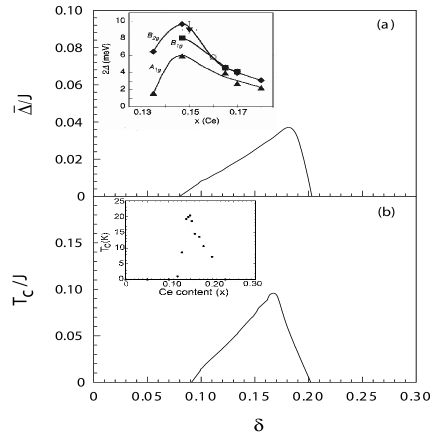
Figure 1: (a) The effective SC gap parameter $\bar{\Delta}$ at $T=0.002J$ and (b) the SC transition temperature $T_{c}$ as a function of the doping concentration for $t/J=-2.5$ and $t^{\prime}/t=0.3$. Inset: the corresponding experimental results of the electron doped cuprate superconductors taken from Refs. [21] and [4].

Now we turn to discuss the electron structure of the electron-doped cuprate superconductors. We have performed a calculation for the electron spectral function (17), and the results of $A({\bf k},\omega)$ in the $[\pi,0]$ point with the doping concentration $\delta=0.11$ (solid line), $\delta=0.13$ (dashed line), and $\delta=0.15$ (dotted line) at $T=0.002J$ for $t/J=-2.5$ and $t^{\prime}/t=0.3$ are plotted in Fig. 2 in comparison with the corresponding experimental result [8] of the electron-doped cuprate superconductor Nd_1.85Ce_0.15CuO₄ (inset). From Fig. 2, we therefore find that there is a sharp SC quasiparticle peak near the electron Fermi energy in the $[\pi,0]$ point. In particular, this electron spectrum is doping dependent. In analogy to the hole-doped case [12], the spectral weight of the SC quasiparticle peak in the electron-doped cuprate superconductors increases with increasing the doping concentration, while the position of the SC quasiparticle peak is shifted towards the Fermi energy. Furthermore, we have discussed the temperature dependence of the electron spectrum, and the results show that the spectral weight of the SC quasiparticle peak decreases as temperature is increased. Our these results are in qualitative agreement with the experimental data [3, 7, 8, 9].

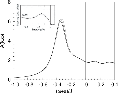
Figure 2: The electron spectral function $A({\bf k},\omega)$ in the $[\pi,0]$ point with $\delta=0.11$ (solid line), $\delta=0.13$ (dashed line), and $\delta=0.15$ (dotted line) at $T=0.002J$ for $t/J=-2.5$ and $t^{\prime}/t=0.3$. Inset: the corresponding experimental result of the electron-doped cuprate superconductor Nd_1.85Ce_0.15CuO₄ taken from Ref. [8].

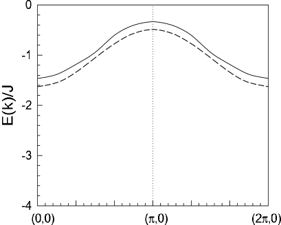
Figure 3: The positions of the lowest energy SC quasiparticle peaks in $A({\bf k},\omega)$ as a function of momentum along the direction $[0,0]\rightarrow[\pi,0]\rightarrow[2\pi,0]$ with $\delta=0.15$ at $T=0.002J$ for $t/J=-2.5$ and $t^{\prime}/t=0.3$. The dashed line is corresponding result [12] of the electron dispersion of the hole-doped cuprate superconductors at $\delta=0.15$ with $T=0.002J$ for parameters $t/J=2.5$ and $t^{\prime}/t=0.3$.

For the further understanding physical properties of the SC quasiparticles near the $[\pi,0]$ point, we have made a series of calculations for $A({\bf k},\omega)$ around the $[\pi,0]$ point, and the results show that as in the hole-doped case, the sharp SC quasiparticle peak in the electron-doped cuprate superconductors persists in a very large momentum space region around the $[\pi,0]$ point. To show this point clearly, we plot the positions of the lowest energy SC quasiparticle peaks in $A({\bf k},\omega)$ as a function of momentum along the direction $[0,0]\rightarrow[\pi,0]\rightarrow[2\pi,0]$ at $\delta=0.15$ with $T=0.002J$ for $t/J=-2.5$ and $t^{\prime}/J=0.3$ in Fig. 3 (solid line). For comparison, the corresponding result [12] of the lowest energy SC quasiparticle peaks in the electron spectral function of the hole-doped cuprate superconductors at $\delta=0.15$ with $T=0.002J$ for $t/J=2.5$ and $t^{\prime}/t=0.3$ is also plotted in Fig. 3 (dashed line). From Fig. 3, it is shown that the sharp SC quasiparticle peaks around the $[\pi,0]$ point at low energies disperse very weakly with momentum, which also is corresponding to the unusual flat band appeared in the normal-state around the $[\pi,0]$ point [22, 23]. In comparison with the hole doped case [12], our results also show explicitly that although the electron-hole asymmetry is observed in the phase diagram [3, 6], the electronic structure of the electron-doped cuprates in the SC state is similar to that in the hole-doped case.

Within the framework of the kinetic energy driven d-wave superconductivity, the essential physics of the electronic structure in the electron-doped cuprate superconductors is the same as that in the hole-doped case [12]. The SC-state of the electron-doped cuprate superconductors is the conventional Bardeen-Cooper-Schrieffer (BCS) like [24], and the SC quasiparticle has the Bogoliubov-quasiparticle nature. This can be understood from the electron diagonal and off-diagonal Green’s functions in Eqs. (15) and (16). As in the hole-doped case [12], the spins center around the $[\pi,\pi]$ point in the MF level [19], therefore the main contributions for the spins comes from the $[\pi,\pi]$ point, where $\omega_{{\bf p}=[\pi,\pi]}\sim 0$. In this case, the electron diagonal and off-diagonal Green’s functions in Eqs. (15) and (16) can be approximately reduced in terms of the self-consistent equation [19] $1/2=\langle S_{i}^{+}S_{i}^{-}\rangle=(1/N)\sum_{{\bf p}}B_{{\bf p}}{\rm coth}(\beta\omega_{{\bf p}}/2)/(2\omega_{{\bf p}})$ as,

$$G({\bf k},\omega) \approx Z_{F}{U_{{\bf k}}^{2}\over\omega-E_{{\bf k}}}+Z_{F}{V_{{\bf k}}^{2}\over\omega+E_{{\bf k}}},$$ (19)

$$\Gamma^{{\dagger}}({\bf k},\omega) \approx Z_{F}{\bar{\Delta}_{aZ}({\bf k})\over 2E_{{\bf k}}}\left({1\over\omega-E_{{\bf k}}}-{1\over\omega+E_{{\bf k}}}\right),$$ (20)

where the electron quasiparticle coherence factors $U^{2}_{{\bf k}}\approx V^{2}_{a{\bf k+k_{A}}}$ and $V^{2}_{{\bf k}}\approx U^{2}_{a{\bf k+k_{A}}}$, the electron quasiparticle spectrum $E_{{\bf k}}\approx E_{a{\bf k+k_{A}}}$, and ${\bf k_{A}}=[\pi,\pi]$, which show that the dressed charge carrier quasiparticle coherence factors $V_{a{\bf k}}$ and $U_{a{\bf k}}$ and quasiparticle spectrum $E_{a{\bf k}}$ have been transferred into the electron quasiparticle coherence factors $U_{{\bf k}}$ and $V_{{\bf k}}$ and quasiparticle spectrum $E_{{\bf k}}$, respectively, by the convolutions of the spin Green’s function and dressed charge carrier diagonal and off-diagonal Green’s functions due to the charge-spin recombination. This also reflects that in the kinetic energy driven SC mechanism, the dressed charge carrier pairs condense with the d-wave symmetry, then the electron Cooper pairs originating from the dressed charge carrier pairing state are due to the charge-spin recombination, and their condensation automatically gives the electron quasiparticle character. This is why the basic BCS formalism [24] is still valid in discussions of the doping dependence of the effective SC gap parameter and SC transition temperature, and the SC coherence of the quasiparticle peak in the electron-doped cuprate superconductors, although the pairing mechanism is driven by the kinetic energy by exchanging spin excitations, and other exotic magnetic scattering [5] is beyond the BCS theory. On the other hand, although there is a similar strength of the magnetic interaction $J$ for both hole-doped and electron-doped cuprates, the interplay of $t^{\prime}$ with $t$ and $J$ causes a further weakening of the AF spin correlation for the hole doping, and enhancing the AF spin correlation for the electron doping [25], which shows that the AF spin correlations in the electron doping is stronger than these in the hole-doped side. This may lead to the charge carrier’s localization over a broader range of doping for the electron doping. As a consequence, the asymmetry of the electron spectrum in the hole-doped and electron-doped cuprates emerges. This is also why superconductivity appears over a narrow range of doping in the electron-doped cuprates. In the normal-state, we [23] have shown within the CSS fermion-spin theory that the lowest energy states are located at the $[\pi,0]$ point for the electron doping, this means that at low doping, the Fermi surface is an electron-pocket centered at the $[\pi,0]$ point, and then further electron doping may lead to the creation of a new holelike Fermi surface centered at the $[\pi,\pi]$ point, in qualitative agreement with the experimental data [9]. As we have mentioned above, the most contributions of the electronic states in the SC-state for the electron doping come from $[\pi,0]$ point [3, 6, 7, 8, 9], and then superconductivity is characterized by an overall d-wave pairing symmetry $\bar{\Delta}({\bf k})=\bar{\Delta}({\rm cos}k_{x}-{\rm cos}k_{y})/2$ [7, 11]. In this case, the d-wave SC gap, and therefore the electron pairing energy scale, is maximized at $[\pi,0]$ point.

In summary, we have discussed the electronic structure of the electron-doped cuprate superconductors based on the kinetic energy driven d-wave SC superconductivity. Our results show explicitly that although the electron-hole asymmetry is observed in the phase diagram, the electronic structure of the electron-doped cuprates in the SC state is similar to that in the hole-doped case. With increasing the electron doping, the spectral weight in the $[\pi,0]$ point increases, while the position of the sharp SC quasiparticle peak is shifted towards the Fermi energy. In analogy to the hole-doped case, the SC quasiparticles around the $[\pi,0]$ point disperse very weakly with momentum.

References

• [1] Y. Tokura, H. Takagi, and S. Uchida, Nature 337, 345 (1989).
• [2] See, e.g., L. Alff, Y. Krockenberger, B. Welter, M. Schonecke, R. Gross, D. Manske, and M. Naito, Nature 422, 698 (2003).
• [3] See, e.g., A. Damascelli, Z. Hussain, and Z.-X. Shen, Rev. Mod. Phys. 75, 475 (2003).
• [4] J.L. Peng, E. Maiser, T. Venkatesan, R.L. Greene, and G. Czjzek, Phys. Rev. B 55, 6145 (1997).
• [5] Stephen D. Wilson, Shiliang Li, Pengcheng Dai, Wei Bao, Jae-Ho Chung, H.J. Kang, Seung-Hun Lee, Seiki Komiya, Yoichi Ando, and Qimiao Si, Phys. Rev. B 74, 144514 (2006); Hyungje Woo, Pengcheng Dai, S. M. Hayden, H. A. Mook, T. Dahm, D. J. Scalapino, T. G. Perring, F. Dogan, Nature Physics 2, 600 (2006).
• [6] See, e.g., Z.X. Shen, and D.S. Dessau, Phys. Rep. 70, 253 (1995), and referenes therein.
• [7] N.P. Armitage, D.H. Lu, D.L. Feng, C. Kim, A. Damascelli, K.M. Shen, F. Ronning, Z.-X. Shen, Y. Onose, Y. Taguchi, and Y. Tokura, Phys. Rev. Lett. 86, 1126 (2001).
• [8] N.P. Armitage, D.H. Lu, C. Kim, A. Damascelli, K.M. Shen, F. Ronning, D.L. Feng, P. Bogdanov, Z.-X. Shen, Y. Onose, Y. Taguchi, Y. Tokura, P.K. Mang, N. Kaneko, and M. Greven, Phys. Rev. Lett. 87, 147003 (2001).
• [9] N.P. Armitage, F. Ronning, D.H. Lu, C. Kim, A. Damascelli, K.M. Shen, D.L. Feng, H. Eisaki, Z.-X. Shen, P.K. Mang, N. Kaneko, M. Greven, Y. Onose, Y. Taguchi, and Y. Tokura, Phys. Rev. Lett. 88, 257001 (2002).
• [10] H. Matsui, K. Terashima, T. Sato, T. Takahashi, M. Fujita, and K. Yamada, Phys. Rev. Lett. 95, 017003 (2005).
• [11] T. Sato, T. Kamiyama, T. Takahashi, K. Kurahashi, and K. Yamada, Science 291, 1517 (2001); C.C. Tsuei and J.R. Kirtley, Phys. Rev. Lett. 85, 182 (2000).
• [12] Huaiming Guo and Shiping Feng, Phys. Lett. A 361, 382 (2007); Shiping Feng and Tianxing Ma, Phys. Lett. A 350, 138 (2006).
• [13] Shiping Feng, Phys. Rev. B 68, 184501 (2003); Shiping Feng, Tianxing Ma, and Huaiming Guo, Physica C 436, 14 (2006); Tianxing Ma, Huaiming Guo, and Shiping Feng, Mod. Phys. Lett. B 18, 895 (2004).
• [14] J. Campuzano, H. Ding, M. Norman, H. Fretwell, M. Randeira, A. Kaminski, J. Mesot, T. Takeuchi, T. Sato, T. Yokoya, T. Takahashi, T. Mochiku, K. Kadowaki, P. Guptasarma, D. Hinks, Z. Konstantinovic, Z. Li, and H. Raffy, Phys. Rev. Lett. 83, 3709 (1999).
• [15] C. Kim, P.J. White, Z.X. Shen, T. Tohyama, Y. Shibata, S. Maekawa, B.O. Wells, Y.J. Kim, R.J. Birgeneau, and M.A. Kastner, Phys. Rev. Lett. 80, 4245 (1998).
• [16] Shiping Feng, Jihong Qin, and Tianxing Ma, J. Phys. Condens. Matter 16, 343 (2004); Shiping Feng, Tianxing Ma, and Jihong Qin, Mod. Phys. Lett. B 17, 361 (2003).
• [17] R.B Laughlin, Phys. Rev. Lett. 79, 1726 (1997); J. Low. Tem. Phys. 99, 443 (1995).
• [18] P.W. Anderson, Phys. Rev. Lett. 67, 2092 (1991); Science 288, 480 (2000).
• [19] Tianxing Ma and Shiping Feng, Phys. Lett. A 339, 131 (2005).
• [20] J. Kondo and K. Yamaji, Prog. Theor. Phys. 47, 807 (1972).
• [21] M.M. Qazilbash, A. Koitzsch, B.S. Dennis, A. Gozar, Hamza Balci, C.A. Kendziora, R.L. Greene, and G. Blumberg, Phys. Rev. B 72, 214510 (2005)
• [22] Z.X. Shen, W.E. Spicer, D.M. King, D.S. Dessau, and B.O. Wells, Science 267, 343 (1995).
• [23] Huaiming Guo and Shiping Feng, Phys. Lett. A 355, 473 (2006).
• [24] J.R. Schrieffer, Theory of Superconductivity, Benjamin, New York, 1964.
• [25] R.J. Gooding, K.J.E. Vos, and P.W. Leung, Phys. Rev. B 50, 12866 (1994); M.S. Hybertson, E. Stechel, M. Schuter, and D. Jennison, Phys. Rev. B 41, 11068 (1990).