Scale-free random branching tree in supercritical phase

Abstract

We study the size and the lifetime distributions of scale-free random branching tree in which $k$ branches are generated from a node at each time step with probability $q_{k}\sim k^{-\gamma}$. In particular, we focus on finite-size trees in a supercritical phase, where the mean branching number $C=\sum_{k}kq_{k}$ is larger than 1. The tree-size distribution $p(s)$ exhibits a crossover behavior when $2<\gamma<3$; A characteristic tree size $s_{c}$ exists such that for $s\ll s_{c}$, $p(s)\sim s^{-\gamma/(\gamma-1)}$ and for $s\gg s_{c}$, $p(s)\sim s^{-3/2}\exp(-s/s_{c})$, where $s_{c}$ scales as $\sim(C-1)^{-(\gamma-1)/(\gamma-2)}$. For $\gamma>3$, it follows the conventional mean-field solution, $p(s)\sim s^{-3/2}\exp(-s/s_{c})$ with $s_{c}\sim(C-1)^{-2}$. The lifetime distribution is also derived. It behaves as $\ell(t)\sim t^{-(\gamma-1)/(\gamma-2)}$ for $2<\gamma<3$, and $\sim t^{-2}$ for $\gamma>3$ when branching step $t\ll t_{c}\sim(C-1)^{-1}$, and $\ell(t)\sim\exp(-t/t_{c})$ for all $\gamma>2$ when $t\gg t_{c}$. The analytic solutions are corroborated by numerical results.

I Introduction

A tree is a graph with no loop within it. Owing to the simplicity of its structure and amenability of analytic studies, tree graph has drawn considerable attentions in many disciplines of scientific researches. Scale-free (SF) random branching tree, in which the number of branches $k$ generated from a node is stochastic following a power-law distribution, $q_{k}\sim k^{-\gamma}$, is particularly interesting here. Such trees can be found in various phenomena such as the trajectories of cascading failure in the sandpile model on SF networks sandpile , epidemic spreading on SF networks epidemic0 ; epidemic1 , aftershock propagation in earthquake earthquake0 ; earthquake1 , random spanning tree or skeleton of SF networks fractal , phylogenetic tree taxanomy , etc. Here, SF network is the network with the degree distribution following a power law $P_{d}(k)\sim k^{-\lambda}$ sf0 ; sf1 ; sf2 . So far, several analytic studies have been performed to understand structural properties of SF branching trees review . However, most works are focused on the critical case, where the mean branching number $C\equiv\sum_{k}kq_{k}$ is equal to 1, motivated by universal feature of scale invariance observed in nature and society.

Recent studies, however, show that the structure of real-world networks may have been designed upon supercritical trees fractal . Supercritical trees, where the mean branching number $C>1$, turn out to act as a skeleton of some fractal networks such as the world-wide web. Here skeleton skeleton is defined as a spanning tree formed by edges with highest betweenness centrality or loads bc ; load . A supercritical branching tree can grow indefinitely with a nonzero probability, which is the most marked difference from critical ($C=1$) or subcritical ($C<1$) tree that cannot grow infinitely. Moreover, the total number of offsprings $s(t)$ generated from a single root (ancestor) up to a given generation $t$ can increase exponentially in supercritical trees and this is reminiscent of the small-world behavior: The mean distance between nodes scales logarithmically as a function of the total number of nodes review .

Due to the mean branching number being larger than 1, some supercritical trees may be alive in a very long time limit. The tree-size distribution of those surviving trees in the supercritical phase has been derived in the mean-field framework rios , which follows a power law, $p(s)\sim s^{-2}$. Here, we consider finite-size trees in the supercritical phase. In spite of the large mean branching number, some trees do not grow infinitely even in the supercritical phase. For such finite-size trees in the supercritical phase, we derive the tree-size and the lifetime distributions using the generating function technique harris . Distinguished from the critical case, the generating function of the tree-size distribution exhibits two singular behaviors in the supercritical phase and thereby a crossover behavior of the tree-size distribution can arise when $2<\gamma<3$. We present in detail the derivation of all these analytic solutions in the following sections. The tree-size and lifetime distributions predicted by analytic solutions are confirmed by numerical simulations. This is important in itself for understanding the branching trees whose structure changes drastically depending on the phase. Since the branching tree approach can be applied to numerous systems, our results should be useful for future diverse applications as well.

II Tree-size distribution

Let us consider the branching process that each node generates $k$ offsprings with probability $q_{k}$,

$$q_{k}=\left\{\begin{array}[]{ll}1-\frac{C\,\zeta(\gamma)}{\zeta(\gamma-1)}&~{}~{}~{}{\rm for}~{}~{}k=0,\\[7.11317pt] \frac{C}{\zeta(\gamma-1)}k^{-\gamma}&~{}~{}~{}{\rm for}~{}~{}k\geq 1,\end{array}\right.$$ (1)

where $C$ is constant in the range of $0<C<\zeta(\gamma-1)/\zeta(\gamma)$ with the Riemann-zeta function $\zeta(x)$, and $\gamma$ is larger than $2$, ensuring that $\zeta(\gamma-1)$ is finite. Then, $C$ is automatically identical to the mean branching number, i.e. the average number of offsprings $C=\sum_{k=0}^{\infty}kq_{k}$ generated from a node. When $C<1$, the number of offsprings decreases on average as branching proceeds and it vanishes eventually. Thus, branching tree has finite lifetime with probability one. When $C>1$, as branching proceeds, the number of offsprings can increase exponentially with non-zero probability. The case of $C=1$ is marginal: Offsprings persist, neither disappear nor flourish on average. A branching tree generated through the stochastic process (1) is a SF branching tree, because its degree distribution follows a power law, $P_{d}(k_{d})\sim k_{d}^{-\gamma}$ asymptotically. Degree $k_{d}$ of each node in the tree is related to the branching number $k$ of that node as $k_{d}=k+1$ but for the root, $k_{d}=k$.

II.1 Generating function method

A tree grows as each of the youngest nodes generates their offsprings following the probability $q_{k}$ in Eq. (1). This evolution is regarded as a process in a unit time step. When a node generates no offspring with probability $q_{0}$, it remains inactive in further time steps. We define $p_{t}(s)$ as the fraction of trees with total number of nodes $s$ at time $t$. By definition, $p_{0}(s)=\delta_{s,1}$. Then, $p_{t+1}(s)$ can be written in terms of $p_{t}(s)$ as

$$p_{t+1}(s)=\sum_{k=0}^{\infty}q_{k}\sum_{s_{1},s_{2},\ldots,s_{k}}p_{t}(s_{1})p_{t}(s_{2})\cdots p_{t}(s_{k})\delta_{\sum_{i=1}^{k}s_{i},s-1}.$$ (2)

Defining the generating functions, $\mathcal{Q}(\omega)=\sum_{k=0}^{\infty}q_{k}\omega^{k}$ and $\mathcal{P}_{t}(y)=\sum_{s=1}^{\infty}p_{t}(s)y^{s}$, and applying them to (2), one can obtain that

$$\mathcal{P}_{t+1}(y)=y\mathcal{Q}(\mathcal{P}_{t}(y)).$$ (3)

Let us consider the tree-size distribution in the $t\to\infty$ limit, i.e., $p(s)=\lim_{t\to\infty}p_{t}(s)$ and its generating function $\mathcal{P}(y)=\lim_{t\to\infty}\mathcal{P}_{t}(y)$. However, some trees may grow infinitely in the supercritical phase, which makes $\mathcal{P}(y)=\sum_{s}p(s)y^{s}$ ill-defined at $y=1$. So we limit the summation in $\mathcal{P}(y)$ over finite trees only, i.e., ${\mathcal{P}}(y)=\sum_{{\rm finite}~{}s}p(s)y^{s}$. This is equivalent to defining ${\cal P}(1)=\lim_{y\to 1}{\mathcal{P}}(y)$. Then, Eq.(3) gives the relation in the $t\to\infty$ limit,

$$\mathcal{P}(y)=y\mathcal{Q}(\mathcal{P}(y)).$$ (4)

The next step is to extract a singular part of $\mathcal{P}(y)$ from Eq. (4), and then to derive the behavior of $p(s)$ for $s\gg 1$.

The power-law form of $q_{k}$ in Eq. (1) results in the expansion of $\mathcal{Q}(\omega)$ around $\omega=1$:

$$\mathcal{Q}(\omega)=1-C(1-\omega)+\frac{B(\gamma)}{2}(1-\omega)^{2}+\cdots$$

$$+\left\{\begin{array}[]{ll}A(\gamma)(1-\omega)^{\gamma-1}&(\gamma\neq{\rm integer})\\[7.11317pt] \frac{(-1)^{\gamma}}{\Gamma(\gamma)}(1-\omega)^{\gamma-1}\ln(1-\omega)&(\gamma={\rm integer})\end{array}\right.+\cdots,$$ (7)

where $B(\gamma)=C[\zeta(\gamma-2)/\zeta(\gamma-1)-1]$, and $A(\gamma)=C\Gamma(1-\gamma)/\zeta(\gamma-1)$ with the Gamma function $\Gamma(x)$. The inverse function $y=\mathcal{P}^{-1}(\omega)$ is then expanded as

$$y = \mathcal{P}^{-1}(\omega)=\frac{\omega}{\mathcal{Q}(\omega)}\sim 1+\Delta(1-\omega)-\frac{B(\gamma)}{2}(1-\omega)^{2}+\cdots$$ (10)

$$- \left\{\begin{array}[]{ll}A(\gamma)(1-\omega)^{\gamma-1}&(\gamma\neq{\rm integer})\\[7.11317pt] \frac{(-1)^{\gamma}}{\Gamma(\gamma)}(1-\omega)^{\gamma-1}\ln(1-\omega)&(\gamma={\rm integer})\end{array}\right.+\cdots,$$

where $\Delta\equiv C-1$. We recall that $\Delta$ is positive (negative) in the supercritical (subcritical) regime and $0$ in the critical case. Here we focus on the supercritical case of $\Delta>0$ and being very small, but the obtained result can be naturally extended to large-$\Delta$ cases.

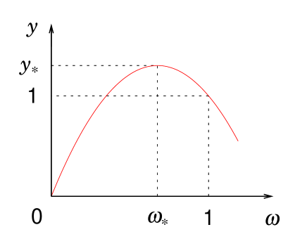
Figure 1: (Color online) Schematic plot of the function $y=\omega/{\cal Q}(\omega)$ in the supercritical phase. The $dy/d\omega=0$ occurs at $\omega=\omega_{*}<1$.

II.2 The singularity at $y=y_{*}>1$

Let us investigate how $y$ behaves as $\omega$ decreases from $1$ to $0$. For $\Delta>0$, as $\omega$ decreases from $1$ to $\omega_{*}$, $y$ increases from $1$ to $y_{*}$ and then decreases to zero as shown in Fig.1, where $\omega_{*}$ satisfying $(d/d\omega)[\omega/\mathcal{Q}(\omega)]|_{\omega=\omega_{*}}=0$ locates less than 1. This feature is distinguished from the solution $\omega_{*}=1$ for the critical case. It is obtained that $\omega_{*}$ depends on $\Delta$ as

$$1-\omega_{*}\equiv\epsilon_{*}\sim\left\{\begin{array}[]{ll}\Delta&{\rm for}~{}~{}~{}\gamma>3,\\[7.11317pt] \Delta/\ln(1/\Delta)&{\rm for}~{}~{}~{}\gamma=3,\\[7.11317pt] \Delta^{1/(\gamma-2)}&{\rm for}~{}~{}~{}2<\gamma<3.\end{array}\right.$$ (11)

The value $y_{*}$, determined by the relation $y_{*}=\omega_{*}/\mathcal{Q}(\omega_{*})$, locates at

$$y_{*}-1\equiv\delta_{*}\sim\left\{\begin{array}[]{ll}\Delta^{2}&{\rm for}~{}~{}~{}\gamma>3,\\[7.11317pt] \Delta^{2}/\ln(1/\Delta)&{\rm for}~{}~{}~{}\gamma=3,\\[7.11317pt] \Delta^{(\gamma-1)/(\gamma-2)}&{\rm for}~{}~{}~{}2<\gamma<3.\end{array}\right.$$ (12)

The curve $y=\omega/\mathcal{Q}(\omega)$ in the region $\omega>\omega_{*}$ is just the analytic continuation of the inverse function $y=\mathcal{P}^{-1}(\omega)$ that is analytic for $\omega<\omega_{*}$ otter .

The right-hand-side of Eq. (10) for $\omega<\omega_{*}$ is expanded around $\omega_{*}$ as

$$y\simeq y_{*}+\sum_{n=2}^{\infty}\frac{D_{n}(\gamma)}{n!}(\omega_{*}-\omega)^{n},$$ (13)

when $\omega$ is close to $\omega_{*}$ such that

$$\max_{n\geq 2}\frac{D_{n+1}(\gamma)}{D_{n}(\gamma)(n+1)}(\omega_{*}-\omega)\ll 1.$$ (14)

Here $D_{n}(\gamma)$ is the $n$th derivative of $\omega/\mathcal{Q}(\omega)$ at $\omega_{*}$. For $n=2$,

$$D_{2}(\gamma)\sim\left\{\begin{array}[]{ll}-B(\gamma)&{\rm for}~{}~{}~{}\gamma>3,\\[7.11317pt] \ln\Delta&{\rm for}~{}~{}~{}\gamma=3,\\[7.11317pt] -\Delta^{(\gamma-3)/(\gamma-2)}&{\rm for}~{}~{}~{}2<\gamma<3.\end{array}\right.$$ (15)

This result is used for future discussions. Keeping only the quadratic term $(\omega_{*}-\omega)^{2}$ in Eq.(13), one obtains the leading singular behavior of ${\mathcal{P}}(y)$ at $y_{*}$,

$$\omega=\mathcal{P}(y)\sim\omega_{*}-\sqrt{\frac{2(y_{*}-y)}{|D_{2}(\gamma)|}}.$$ (16)

In fact such a square-root singularity at $y=y_{*}$ is generic regardless of the form of the branching probability when $q_{0}+q_{1}<1$ otter , yielding the asymptotic behavior of $p(s)$ given by

$$p(s)\sim b(\Delta)s^{-3/2}\exp(-s/s_{*}),$$ (17)

where the coefficient $b(\Delta)\sim\Delta^{-(\gamma-3)/[2(\gamma-2)]}$ for $2<\gamma<3$, $1/\sqrt{\ln(1/\Delta)}$ for $\gamma=3$ and constant for $\gamma>3$, and $s_{*}=(\ln y_{*})^{-1}$.

II.3 The singularity at $y=1$

When $\omega$ is far from $\omega_{*}$ such that the linear term with the coefficient $\Delta$ is not comparable to the next-order term, another singularity becomes dominant. The next-order term is the quadratic term for $\gamma>3$ and the non-analytic term for $2<\gamma\leq 3$. To be precise, if the condition, $1-\omega\gg\Delta$ for $\gamma>3$, $-(1-\omega)\ln(1-\omega)\gg\Delta$ for $\gamma=3$, and $1-\omega\gg\Delta^{1/(\gamma-2)}$ for $2<\gamma<3$, holds, then the linear term is negligible compared with the next order terms, and then Eq.(10) is reduced to

$$y\sim 1-\left\{\begin{array}[]{ll}\frac{B(\gamma)}{2}(1-\omega)^{2}&{\rm for}~{}~{}~{}\gamma>3,\\[7.11317pt] -\frac{1}{2}(1-\omega)^{2}\ln(1-\omega)&{\rm for}~{}~{}~{}\gamma=3,\\[7.11317pt] A(\gamma)(1-\omega)^{\gamma-1}&{\rm for}~{}~{}~{}2<\gamma<3.\end{array}\right.$$ (18)

The generating function $\mathcal{P}(y)$ then behaves as

$$\omega=\mathcal{P}(y)\sim 1-\left\{\begin{array}[]{ll}\sqrt{\frac{2(1-y)}{B(\gamma)}}&{\rm for}~{}~{}~{}\gamma>3,\\[7.11317pt] \sqrt{\frac{4(1-y)}{|\ln(1-y)|}}&{\rm for}~{}~{}~{}\gamma=3,\\[7.11317pt] \left(\frac{1-y}{A(\gamma)}\right)^{1/(\gamma-1)}&{\rm for}~{}~{}~{}2<\gamma<3.\end{array}\right.$$ (19)

From this result, one can obtain the tree-size distribution as

$$p(s)\sim\left\{\begin{array}[]{ll}s^{-3/2}&{\rm for}~{}~{}~{}\gamma>3,\\[7.11317pt] s^{-3/2}(\ln s)^{-1/2}&{\rm for}~{}~{}~{}\gamma=3,\\[7.11317pt] s^{-\gamma/(\gamma-1)}&{\rm for}~{}~{}~{}2<\gamma<3.\end{array}\right.$$ (20)

II.4 Crossover behavior between the two singularities

The two singular behaviors of $\mathcal{P}(y)$ in the forms of Eqs. (16) and (19) occurring at $y=y_{*}$ and $y=1$, respectively, enables us to determine the ranges of size $s$ where the formulae of Eqs.(17) and (20) are valid. In particular, when $2<\gamma\leq 3$, the asymptotic behaviors in Eqs.(17) and (20) differs from each other and thus there should be a crossover behavior in the tree-size distribution.

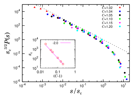
Figure 2: (Color online) The tree-size distribution $p(s)$ for $\gamma=3.3$ for various values of $C$ in the scaling form Eq. (21). Dashed line is guideline with a slope of $-3/2$. Inset: Dependence of the characteristic size $s_{c}$ on the mean branching number $C$.

The ranges of $\omega$ in which Eqs. (13) and (18) are valid are closely related to those of $y$ for Eqs. (16) and (19) and that of $s$ for Eqs. (17) and (20), respectively. Here we find those ranges of $\omega$, $y$, and $s$, and then determine the crossover in the tree-size distribution $p(s)$.

First, we study valid ranges of Eqs. (13), (16), and (17). The coefficient $D_{n}(\gamma)$ in Eq. (13) behaves as $\sim(1-\omega_{*})^{\gamma-1-n}$ for $n>\gamma-1$ due to the non-analytic term $(1-\omega)^{\gamma-1}$ in Eq. (10) when $\gamma$ is not integer. Then, it follows that $[D_{n}(\gamma)(n+1)/D_{n+1}(\gamma)]\sim 1/(1-\omega_{*})\equiv 1/\epsilon_{*}$. Thus, the condition (14) can be rewritten as $\omega_{*}-\epsilon_{c}^{>}\ll\omega<\omega_{*}$, where $\epsilon_{c}^{>}\sim\Delta$ for $\gamma>3$, $\epsilon_{c}^{>}\sim\Delta/\ln(1/\Delta)$ for $\gamma=3$, and $\epsilon_{c}^{>}\sim\Delta^{1/(\gamma-2)}$ for $2<\gamma<3$ from Eq.(11). The corresponding range of $y$ is $y_{*}-\delta_{c}^{>}\ll y<y_{*}$, where $\delta_{c}^{>}$ is given by $\sim\Delta^{2}$ for $\gamma>3$, $\sim\Delta^{2}/\ln(1/\Delta)$ for $\gamma=3$, and $\sim\Delta^{(\gamma-1)/(\gamma-2)}$ for $2<\gamma<3$ by using Eqs.(12) and (16).

To find valid range of $s$ for $p(s)$ in Eq.(17), we use the fact that the singular functional behavior of $\mathcal{P}(y)$ around $y=\tilde{y}$ is determined by that of $p(s)$ around $s=\tilde{s}$, where $\tilde{y}$ and $\tilde{s}$ are related as $\tilde{y}^{\tilde{s}}\sim 1$. Then, one can find that $s_{c}^{>}=|\ln(y_{*}-\delta_{c}^{>})|^{-1}\sim(\delta_{*}-\delta_{c}^{>})^{-1}$, so that $s_{c}^{>}\sim\Delta^{-2}$ for $\gamma>3$, $\Delta^{-2}\ln(1/\Delta)$ for $\gamma=3$, and $\Delta^{-(\gamma-1)/(\gamma-2)}$ for $2<\gamma<3$. For the range $s\gg s_{c}^{>}$, the formula (17) is valid.

Second, we check the validities of Eqs. (18), (19), and (20). Comparing the magnitude of the linear term and the next-order term in Eq. (10), we find that Eq. (18) is valid for $\omega\ll 1-\epsilon_{c}^{<}$, where $\epsilon_{c}$ behaves as $\Delta$ for $\gamma>3$, $\Delta/\ln(1/\Delta)$ for $\gamma=3$, and $\Delta^{1/(\gamma-2)}$ for $2<\gamma<3$. The corresponding range of $y$ for Eq. (19) is given as $y\ll 1-\delta_{c}^{<}$, where $\delta_{c}^{<}\sim\Delta^{2}$ for $\gamma>3$, $\delta_{c}^{<}\sim\Delta^{2}/\ln(1/\Delta)$ for $\gamma=3$, and $\delta_{c}^{<}\sim\Delta^{(\gamma-1)/(\gamma-2)}$ for $2<\gamma<3$. The corresponding range of $s$ for Eq. (20) is $s\ll s_{c}^{<}$ with $s_{c}^{<}=|\ln(1-\delta_{c}^{<})|^{-1}\sim(\delta_{c}^{<})^{-1}$ given by $s_{c}^{<}\sim\Delta^{-2}$ for $\gamma<3$, $s_{c}^{<}\sim\Delta^{-2}\ln(1/\Delta)$ for $\gamma=3$, and $s_{c}^{<}\sim\Delta^{-(\gamma-1)/(\gamma-2)}$ for $2<\gamma<3$.

As already noticed, the crossover sizes $s_{c}^{>}$, $s_{c}^{<}$, and $s_{*}$ are consistent for all values of $\gamma$ within $\Delta$-dependence, and thereby, we use the notation $s_{c}$ for all of them. The overall behavior of the tree-size distribution is obtained by combining Eqs. (17) and (20). For $\gamma>3$, there is no need to introduce a crossover. Thus, it leads to

$$p(s)\sim s^{-3/2}\exp(-s/s_{c})\quad(\gamma>3),$$ (21)

for all $s$. And $s_{c}\sim\Delta^{-2}$. As $\Delta$ increases, the cut-off $s_{c}$ decreases and the exponential-decaying pattern prevails.

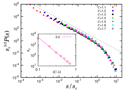
Figure 3: (Color online) The tree-size distribution $p(s)$ for $\gamma=2.5$ for various values of $C$ in the scaling form Eq. (23). Dashed line is guideline with a slope of $-5/3$. Inset: Dependence of the characteristic size $s_{c}$ on the mean branching number $C$.

When $\gamma=3$, $p(s)$ is given by

$$p(s)\sim\left\{\begin{array}[]{ll}s^{-3/2}(\ln s)^{-1/2}&{\rm for}\ s\ll s_{c},\\[7.11317pt] s^{-3/2}\exp(-s/s_{c})&{\rm for}\ s\gg s_{c},\end{array}\right.\quad(\gamma=3)$$ (22)

where $s_{c}\sim\Delta^{-2}\ln(1/\Delta)$. Similarly, for $2<\gamma<3$, we find that

$$p(s)\sim\left\{\begin{array}[]{ll}s^{-\gamma/(\gamma-1)}&{\rm for}\ s\ll s_{c},\\[7.11317pt] s^{-3/2}\exp(-s/s_{c})&{\rm for}\ s\gg s_{c},\end{array}\right.\quad(2<\gamma<3)$$ (23)

where both $s_{c}\sim\Delta^{-(\gamma-1)/(\gamma-2)}$. As $\Delta\to 0$, $s_{c}$ diverges, and the power-law behavior prevails.

We invoke numerical simulations to confirm our analytic solutions. Figs. 2 and 3 show the tree size distributions for $\gamma=3.3$ and $\gamma=2.5$ in the scaling forms, Eq. (21) and Eq. (23), respectively. The data are well collapsed into the predicted formulas for different $C$ values for both cases.

III Lifetime distribution

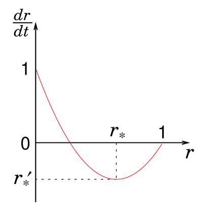
Figure 4: (Color online) Schematic plot of the function $dr/dt={\cal Q}(r)-r$ in the supercritical phase. $(\partial/\partial r)(dr/dt)=0$ occurs at $r_{*}$, at which $dr/dt$ is denoted as $r_{*}^{\prime}$.

Next we solve the lifetime distribution $\ell(t)$. This is defined as the probability that the branching process stops at $t$. To derive $\ell(t)$, we first introduce the probability that the branching process stops at or prior to time $t$, denoted by $r(t)$. Then $\ell(t)$ is given as $\ell(t)=r(t+1)-r(t)$. The probability distribution $r(t)$ is related to $r(t-1)$ as

$$r(t)=\sum_{k=0}^{\infty}q_{k}[r(t-1)]^{k}=\mathcal{Q}(r(t-1)).$$ (24)

Thus, we are given approximately a differential equation for $r(t)$,

$$\frac{dr(t)}{dt}\approx\ell(t)=\mathcal{Q}(r(t))-r(t),$$ (25)

Expanding the right hand side of Eq. (25) around $r=1$, one can see its asymptotic behavior. Using Eq. (7) again, we find $dr/dt$ in the long time limit as follows:

$$\frac{dr}{dt} = \mathcal{Q}(r)-r=-\Delta(1-r)+\frac{B(\gamma)}{2}(1-r)^{2}+\cdots$$ (28)

$$+ \left\{\begin{array}[]{ll}A(\gamma)(1-r)^{\gamma-1}&(\gamma\neq{\rm integer})\\[7.11317pt] \frac{(-1)^{\gamma}}{\Gamma(\gamma)}(1-r)^{\gamma-1}\ln(1-r)&(\gamma={\rm integer})\end{array}\right.+\cdots.$$

What we can see in this relation is that the value of $r^{\prime}$ is zero at $r=1$. It decreases as $r$ decreases until it reaches $r_{*}$ where $(d/dr)[\mathcal{Q}(r)-r]|_{r=r_{*}}=0$ holds. Passing $r_{*}$, $r^{\prime}$ increases as $r$ decreases further, crossing the $r^{\prime}=0$ as shown in Fig. 4.

First, as in the case of $\omega/\mathcal{Q}(\omega)$, two singularities exist in $\mathcal{Q}(r)-r$. For $r$ close to $r_{*}$, Eq. (28) is expanded as

$$r^{\prime}\simeq r^{\prime}_{*}+\sum_{n=2}^{\infty}\frac{G_{n}(\gamma)}{n!}(r_{*}-r)^{n},$$ (29)

where $r^{\prime}_{*}=\mathcal{Q}(r_{*})-r_{*}<0$ and $G_{n}(\gamma)$ is the $n$-th derivative of $\mathcal{Q}(r)-r$ at $r^{*}$. When $r$ is close to $r_{*}$ such that

$${\rm{max}}_{n\geq 2}\frac{G_{n+1}(\gamma)}{G_{n}(\gamma)(n+1)}(r_{*}-r)\ll 1,$$ (30)

one may neglect higher order terms, keeping only the quadratic term in $r_{*}-r$ as

$$\frac{dr}{dt}\approx r^{\prime}_{*}+\frac{G_{2}(\gamma)}{2}(r_{*}-r)^{2}.$$ (31)

The solution to the above differential equation is

$$r(t)\simeq r(\infty)-\frac{2a}{e^{t/t_{*}}-1},$$ (32)

where $r(\infty)=r_{*}-a$ and $a=\sqrt{{2|r^{\prime}_{*}|}/{G_{2}(\gamma)}}$, and $t_{*}=1/\sqrt{2|r^{\prime}_{*}|G_{2}(\gamma)}$. The lifetime distribution $\ell(t)=r^{\prime}(t)$ is then given by

$$\ell(t)\simeq\frac{2ae^{t/t_{*}}}{t_{*}(e^{t/t_{*}}-1)^{2}}\sim\frac{2a}{t_{*}}e^{-t/t_{*}}.$$ (33)

Second, following the same steps taken for the singularities of $\mathcal{P}(y)$, we find another approximate relation between $r^{\prime}$ and $r$ in the region of $r(t)$ where the next order term in Eq. (28) is much larger than its linear term as follows:

$$\frac{dr}{dt}\sim\left\{\begin{array}[]{ll}\frac{B(\gamma)}{2}(1-r)^{2}&{\rm for}~{}~{}~{}\gamma>3,\\[7.11317pt] -\frac{1}{2}(1-r)^{2}\ln(1-r)&{\rm for}~{}~{}~{}\gamma=3,\\[7.11317pt] A(\gamma)(1-r)^{\gamma-1}&{\rm for}~{}~{}~{}2<\gamma<3.\end{array}\right.$$ (34)

Their solutions are, in long time limit, given by

$$1-r(t)\sim\left\{\begin{array}[]{ll}t^{-1}&{\rm for}~{}~{}~{}\gamma>3,\\[7.11317pt] t^{-1}(\ln t)^{-1}&{\rm for}~{}~{}~{}\gamma=3,\\[7.11317pt] t^{-1/(\gamma-2)}&{\rm for}~{}~{}~{}2<\gamma<3.\end{array}\right.$$ (35)

From these results, the lifetime distributions are obtained as

$$\ell(t)\sim\left\{\begin{array}[]{ll}t^{-2}&{\rm for}~{}~{}~{}\gamma>3,\\[7.11317pt] t^{-2}(\ln t)^{-1}&{\rm for}~{}~{}~{}\gamma=3,\\[7.11317pt] t^{-(\gamma-1)/(\gamma-2)}&{\rm for}~{}~{}~{}2<\gamma<3.\end{array}\right.$$ (36)

Different behaviors of the lifetime distribution shown in Eqs. (33) and (36) suggest the presence of a crossover behavior. The characteristic time that distinguishes the two behaviors for given $\gamma$ can be found by considering the valid ranges of $t$ for Eqs. (33) and (36), respectively. When the condition of Eq. (30) is fulfilled, Eqs. (32) and (33) are valid. The condition is approximately represented in different form of $r_{*}-r\ll 1-r_{*}$ since $G_{n}(\gamma)\sim(1-r_{*})^{\gamma-1-n}$. From Eq. (28), one can find the value of $1-r_{*}$ for different $\gamma$’s: $1-r_{*}\sim\Delta$ for $\gamma>3$, $\Delta/\ln(1/\Delta)$ for $\gamma=3$, and $\Delta^{1/(\gamma-2)}$ for $2<\gamma<3$, respectively. Applying these conditions to Eq. (32), it is found that Eqs. (32) and (33) are valid if $t\gg t_{*1}$ with $t_{*1}\sim\Delta^{-1}$ irrespective of $\gamma$ as long as $\gamma>2$.

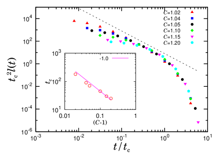
Figure 5: (Color online) The lifetime distribution $\ell(t)$ for $\gamma=3.3$ in the scaling form Eqs. (37) and (38). Dashed line is guideline with slope $-2$. Data for small $t$ are deviated from the data collapse, indicating that our solution is valid for large $t$ only. Inset: Dependence of the characteristic time $t_{c}$ on the mean branching number $C$.

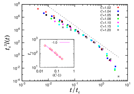
Figure 6: (Color online) The lifetime distribution $\ell(t)$ for $\gamma=2.5$ in the scaling form Eqs. (37) and (38). Dashed line is guideline with slope $-3$. Data for small $t$ are deviated from the data collapse, indicating that our solution is valid for large $t$ only. Inset: Dependence of the characteristic time $t_{c}$ on the mean branching number $C$.

Eqs. (35) and (36) are valid when the linear term is much smaller than the next order term, which is satisfied when $1-r\gg\Delta$ for $\gamma>3$, $1-r\gg\Delta/\ln(1/\Delta)$ for $\gamma=3$, and $1-r\gg\Delta^{1/(\gamma-2)}$ for $2<\gamma<3$, respectively. Applying these conditions to Eq. (35) leads commonly to $t\ll t_{*2}\sim\Delta^{-1}$. One can find that the two characteristic times $t_{*1}$ and $t_{*2}$, and $t_{*}$ scale in the same manner, so that they are denoted as $t_{c}$ commonly. Therefore, we conclude that the lifetime distribution behaves as

$$\ell(t)\sim\left\{\begin{array}[]{ll}t^{-2}&{\rm for}~{}~{}~{}\gamma>3,\\[7.11317pt] t^{-2}(\ln t)^{-1}&{\rm for}~{}~{}~{}\gamma=3,\\[7.11317pt] t^{-(\gamma-1)/(\gamma-2)}&{\rm for}~{}~{}~{}2<\gamma<3,\end{array}\right.$$ (37)

when $t\ll t_{c}\sim\Delta^{-1}$, and

$$\ell(t)\sim e^{-t/t_{c}}~{}~{}~{}~{}~{}~{}~{}{\rm for}~{}~{}~{}\gamma>2$$ (38)

when $t\gg t_{c}$. The analytic solutions for the lifetime distribution are checked by numerical simulations in Figs. 5 and 6. Data in small $t$ regime are somewhat deviated from the data-collapsed formula, indicating that our solution is valid in large $t$ regime.

IV Conclusions and Discussion

Our main results are Eqs. (21), (22), and (23) for the tree-size distribution when trees are finite: Contrary to the case of $\gamma>3$ for which the tree-size distribution $p(s)$ behaves as $\sim s^{-3/2}\exp(-s/s_{c})$ for all $s$ with $s_{c}\sim(C-1)^{-2}$, a crossover behavior occurs at $s_{c}\sim(C-1)^{-(\gamma-1)/(\gamma-2)}$ for $2<\gamma<3$. For $s\ll s_{c}$, $p(s)\sim s^{-\gamma/(\gamma-1)}$ and for $s\gg s_{c}$, $p(s)\sim s^{-3/2}\exp(-s/s_{c})$. This result is complementary to the previous mean-field solution $p_{\rm inf}(s)\sim s^{-2}$ for infinite-size tree. From our solutions, it is noteworthy that the characteristic size $s_{c}$ increases as the exponent $\gamma$ approaches 2. This leads to an interesting result: A larger-size tree can be generated for smaller value of the exponent $\gamma$. However, the probability to have such a large-size tree becomes smaller as the exponent $\gamma$ approaches 2, because the exponent $\gamma/(\gamma-1)$ for the tree-size distribution $p(s)$ becomes larger.

The lifetime distribution also exhibits a crossover behavior at $t_{c}\sim(C-1)^{-1}$. It follows Eq. (37) for $t\ll t_{c}$ and (38) for $t\gg t_{c}$.

This work was supported by KRF Grant No. R14-2002-059-010000-0 of the ABRL program funded by the Korean government (MOEHRD). Notre Dame’s Center for Complex Networks kindly acknowledges the support of the National Science Foundation under Grant No. ITR DMR-0426737.

References

- (1) K.-I. Goh, D.-S. Lee, B. Kahng, and D. Kim, Phys. Rev. Lett. 91, 148701 (2003).
- (2) R. Pastor-Satorras and A. Vespignani, Phys. Rev. Lett. 86, 3200 (2001).
- (3) M.E.J. Newman, Phys. Rev. E 66, 016128 (2002).
- (4) A. Saichev, A. Helmstetter and D. Sornette, Pure appl. geophys. 162, 1113 (2005).
- (5) M. Baiesi and M. Paczuski, Phys. Rev. E 69, 066106 (2004).
- (6) K.-I. Goh, G. Salvi, B. Kahng, and D. Kim, Phys. Rev. Lett. 96, 018701 (2006); J.S. Kim, K.-I. Goh, G. Salvi, E. Oh, B. Kahng and D. Kim, arXiv:cond-mat/0605324.
- (7) G. Caldarelli, C.C. Cartozo, P. De Los Rios and V.D.P. Servedio, Phys. Rev. E 69, 035101(R) (2004).
- (8) R. Albert abd A.-L. Barabási, Rev. Mod. Phys. 74, 47 (2002).
- (9) M.E.J. Newman, SIAM Rev. 45, 167 (2003).
- (10) S. Boccaletti, V. Latora, Y. Moreno, M. Chavez, and D.U. Hwang, Phys. Rep. 424, 175 (2006).
- (11) L. Donetti and C. Destri, J. Phys. A: Math. Gen. 37, 6003 (2004).
- (12) D.-H. Kim, J.D. Noh and H. Jeong, Phys. Rev. E 70, 046126 (2004).
- (13) L.C. Freeman, Sociometry 40, 35 (1977).
- (14) K.-I. Goh, B. Kahng, and D. Kim, Phys. Rev. Lett. 87, 278701 (2001).
- (15) P. De Los Rios, Europhys. Lett. 56, 898 (2001).
- (16) T.E. Harris, The Theory of Branching Processes (Springer-Verlag, Berlin, 1963).
- (17) R. Otter, Ann. Math. Stat. 20, 206 (1949).