Negative magnetic susceptibility and nonequivalent ensembles for the
mean-field $\bm{\phi^{4}}$ spin model

Abstract

We calculate the thermodynamic entropy of the mean-field $\phi^{4}$ spin model in the microcanonical ensemble as a function of the energy and magnetization of the model. The entropy and its derivative are obtained from the theory of large deviations, as well as from Rugh’s microcanonical formalism, which is implemented by computing averages of suitable observables in microcanonical molecular dynamics simulations. Our main finding is that the entropy is a concave function of the energy for all values of the magnetization, but is nonconcave as a function of the magnetization for some values of the energy. This last property implies that the magnetic susceptibility of the model can be negative when calculated microcanonically for fixed values of the energy and magnetization. This provides a magnetization analog of negative heat capacities, which are well-known to be associated in general with the nonequivalence of the microcanonical and canonical ensembles. Here, the two ensembles that are nonequivalent are the microcanonical ensemble in which the energy and magnetization are held fixed and the canonical ensemble in which the energy and magnetization are fixed only on average by fixing the temperature and magnetic field.

I Introduction

The Legendre transform connecting the entropy function of the microcanonical ensemble and the free energy of the canonical ensemble in the thermodynamic limit of these ensembles is often used in practice to obtain the entropy of a system from the knowledge of its free energy. Unfortunately, as has been stressed repeatedly in studies of systems involving long-range interactions Gross (1997, 2001); Eyink and Spohn (1993); Ellis et al. (2000); Dauxois et al. (2002); Touchette et al. (2004), the entropy is the Legendre transform of the free energy only if the entropy is concave as a function of the energy. If the entropy is a nonconcave function of the energy, as it often happens in long-range systems, then it cannot be calculated as the Legendre transform of the free energy. In this case, one must resort to analytically obtain the entropy by other means, e.g., by evaluating directly the density of states from which the entropy is defined (see, e.g., Refs. Ispolatov and Cohen (2000); Barré et al. (2001)), or by using large deviation techniques based on the microcanonical ensemble Ellis et al. (2000, 2004); Costeniuc et al. (2005a); Barré et al. (2005); Hahn and Kastner (2006). Another possibility put forward recently works by modifying the definition of the canonical ensemble in such a way that nonconcave entropies can be obtained from the Legendre transform of a modified form of free energy Costeniuc et al. (2005b, 2006a). Examples of applications of this generalized canonical ensemble can be in found in Refs. Touchette and Beck (2006); Costeniuc et al. (2006b).

There are many types of statistical models whose entropy is known to be a nonconcave function of the energy. Examples, listed in the order in which they were discovered, include systems of particles interacting through gravitational forces Lynden-Bell and Wood (1968); Thirring (1970); Chavanis (2002); Chavanis and Ispolatov (2002), a model of plasma Smith and O’Neil (1990), statistical models of two-dimensional turbulence Kiessling and Lebowitz (1997); Ellis et al. (2002), as well as several spin models involving long-range and mean-field interactions Ispolatov and Cohen (2000); Barré et al. (2001); Ellis et al. (2004); Costeniuc et al. (2005a). Our goal in this paper is to study yet another model, which departs somewhat from the models listed above in that its microcanonical entropy is nonconcave as a function of its energy and magnetization. This, as we shall see, has many consequences for the equivalence of the many different ensembles that can be conceived for this model according to whether the energy and magnetization are treated in a canonical or microcanonical way, i.e., whether these quantities are assumed to fluctuate or not. Parallels between these cases of nonequivalent ensembles and those studied in the context of the energy alone will be discussed. In particular, we shall see that one consequence of the nonconcavity of the entropy with the added magnetization is that the magnetic susceptibility of the model, calculated microcanonically, can be negative. The parallel for systems having nonconcave entropies as a function of the energy is that the heat capacity can be negative Lynden-Bell and Wood (1968); Thirring (1970); Gross (1997, 2001); Lynden-Bell (1999); Touchette (2003).

The possibility for the entropy to be nonconcave in a variable other than the energy or in more than one variable is discussed by Ellis, Haven and Turkington Ellis et al. (2000) in the context of their general theory of nonconcave entropies and nonequivalent ensembles. These authors presented in Ref. Ellis et al. (2002) a first application of their theory for a statistical model of two-dimensional turbulence, whose entropy is nonconcave as a function of the energy and circulation. A model similar to the one treated here having a nonconcave entropy as a function of its energy and magnetization was also studied recently by Hahn and Kastner in Refs. Hahn and Kastner (2005, 2006). What we present here can be seen as a continuation and an extension of these papers. The difference with Refs. Hahn and Kastner (2005, 2006) is that we present not one but two methods for calculating the entropy as a function of the energy and magnetization: one based on large deviation theory and a second based on Rugh’s microcanonical formalism Rugh (1998, 2001). Additionally, we discuss some of the relationships that exist between the nonconcavity of the entropy, the nonequivalence of the microcanonical and canonical ensembles, and the appearance of first-order phase transitions in the canonical ensemble.

II The model and its thermodynamic description

The model that we study in this paper is the so-called mean-field $\phi^{4}$ model, defined by the Hamiltonian

$$H=\sum_{i=1}^{N}\left(\frac{p_{i}^{2}}{2}-\frac{1}{4}q_{i}^{2}+\frac{1}{4}q_{i}^{4}\right)-\frac{1}{4N}\sum_{i,j=1}^{N}q_{i}q_{j}.$$ (1)

In this expression, $q_{i}$ and $p_{i}$ are the canonical coordinates of unit mass particles moving on a line ($q_{i},p_{i}\in\mathbb{R}$). These particles are subjected to a local double-well potential, in addition to interact with each other through a mean-field (infinite range) interaction given by the all-to-all coupling in the double sum. In the following, we shall use $x$ to denote a point of the phase space $\Gamma$ of the system, i.e., $x=(\{p_{i}\},\{q_{i}\})$.

The mean-field $\phi^{4}$ model was introduced by Desai and Zwanzig Desai and Zwanzig (1978) who studied its relaxation to equilibrium using Langevin dynamics. More recently, Dauxois, Lepri and Ruffo Dauxois et al. (2003) have studied this model in the canonical ensemble, and showed that it exhibits a second-order ferromagnetic phase transition. The critical temperature of the transition is found to be $T_{c}\approx 0.264$, corresponding to a critical energy per particle or mean energy $\varepsilon_{c}=T_{c}/2\approx 0.132$. The steps leading to the calculation of the entropy of the mean-field $\phi^{4}$ model augmented by an extra magnetic field were also presented recently by two of us in Ref. Campa and Ruffo (2006). In the same paper, molecular dynamics simulations performed above the critical energy are reported in an attempt to study the convergence of finite-$N$ averages calculated in Rugh’s microcanonical formalism. Finally, as mentioned in the introduction, Hahn and Kastner Hahn and Kastner (2005, 2006) have studied a mean-field $\phi^{4}$ model similar to the one studied here. They have calculated for their model the thermodynamic entropy as a function of the mean energy $\varepsilon(x)=H(x)/N$ and the mean magnetization, defined as

$$m(x)=\frac{1}{N}\sum_{i=1}^{N}q_{i}.$$ (2)

We recall that, in terms of these two quantities, the definition of the entropy is

$$s(\varepsilon,m)=\lim_{N\rightarrow\infty}\frac{1}{N}\ln\int_{\Gamma}\delta(\varepsilon(x)-\varepsilon)\delta(m(x)-m)dx.$$ (3)

Naturally, in terms of $\varepsilon$ alone, we have

$$s(\varepsilon)=\lim_{N\rightarrow\infty}\frac{1}{N}\ln\int_{\Gamma}\delta\left(\varepsilon(x)-\varepsilon\right)dx.$$ (4)

Our goal in the next sections is to calculate $s(\varepsilon,m)$ for the Hamiltonian defined in (1). In doing so, we shall try to highlight the difficulties that arise in calculating this function due to the fact that it is nonconcave, in addition to discuss the physical consequences of having a nonconcave entropy in two thermodynamic variables. The fundamental difficulty, for what concerns calculations, is basically the following. If $s(\varepsilon,m)$ were concave, then we could calculate this function from the point of view of the canonical ensemble using the following steps:

(i) Calculate the partition function

$$Z(\beta,\eta)=\int_{\Gamma}e^{-\beta H(x)-\eta M(x)}dx,$$ (5)

where $M(x)=Nm(x)$ is the total magnetization.

(ii) Calculate the thermodynamic free energy function of the model defined by

$$\varphi(\beta,\eta)=-\lim_{N\rightarrow\infty}\frac{1}{N}\ln Z(\beta,\eta).$$ (6)

(iii) Obtain $s(\varepsilon,m)$ by taking the Legendre transform of free energy function $\varphi(\beta,\eta)$; in symbols,

$$s(\varepsilon,m)=\beta\varepsilon+\eta m-\varphi(\beta,\eta),$$ (7)

with $\beta$ and $\eta$ determined by the equations

$$\frac{\partial}{\partial\beta}\varphi(\beta,\eta)=\varepsilon,\quad\frac{\partial}{\partial\eta}\varphi(\beta,\eta)=m.$$ (8)

The problem with nonconcave entropies is that the last step does not actually yield the correct entropy function because Legendre transforms yield only concave functions. To circumvent this problem, we proceed in the next section to obtain $s(\varepsilon,m)$ using another method suggested by large deviations Ellis et al. (2000). The method is the same as that used in Refs. Hahn and Kastner (2005, 2006); Campa and Ruffo (2006) (see also Refs. Ellis et al. (2004); Costeniuc et al. (2005a); Barré et al. (2005)). The results obtained will then be compared with those derived with Rugh’s method. This second method is the subject of Sec. IV. The results obtained by the two methods are reported, compared and discussed in Sec. V.

Before we jump to the next section, it is useful to note that the partition function shown in (5) can be re-written in the more familiar form

$$Z(\beta,h)=\int_{\Gamma}e^{-\beta[H(x)-hM(x)]}dx$$ (9)

by defining $\eta=-\beta h$. This shows that the partition function defined in (5) is nothing but the standard, canonical partition function of $H$ with an added external magnetic field $h$. As is well known, $h$ is the field of the canonical ensemble which is conjugated to the magnetization constraint $m(x)=m$ of the microcanonical ensemble, while $\beta$ is the canonical field conjugated to the microcanonical energy constraint $\varepsilon(x)=\varepsilon$. These observations are important for what is coming later.

III Large deviation calculation of the entropy

The large deviation method described in this section is essentially a generalization of the maximum entropy principle, which is particularly suited for many-particle systems involving long-range or mean-field interactions. The method is presented in detail in Ref. Ellis et al. (2000), and was used recently to calculate the entropy function of many models; see, e.g., Refs. Ellis et al. (2004); Costeniuc et al. (2005a); Barré et al. (2005).

The basic ingredients of the method are the following. First, one must be able to find a set of macro-variables or “mean fields”, denoted collectively by the vector $\mu(x)$, which are such that the energy per particle $\varepsilon(x)$ and the mean magnetization $m(x)$ can be re-written as a function of these variables. In symbols, this means that there must exist two functions $\tilde{\varepsilon}$ and $\tilde{m}$ of $\mu$ such that

$$\varepsilon(x)=\tilde{\varepsilon}(\mu(x)),\quad m(x)=\tilde{m}(\mu(x)).$$ (10)

(See Ref. Ellis et al. (2000) or Ellis et al. (2004) for a more complete and more accurate statement of this condition.) Second, one must be able to derive the expression of the entropy function $\tilde{s}(\mu)$ for the macrostate $\mu$, which, in analogy with $s(\varepsilon)$ and $s(\varepsilon,m)$, is defined as

$$\tilde{s}(\mu)=\lim_{N\rightarrow\infty}\frac{1}{N}\ln\int_{\Gamma}\delta(\mu(x)-\mu)dx.$$ (11)

In large deviation theory, the function $\tilde{s}(\mu)$ is interpreted as the rate function (up to a sign) governing the fluctuations of $\mu$ with respect to the probability measure defining the microcanonical ensemble Ellis et al. (2000). With this function, we finally obtain the entropy $s(\varepsilon,m)$ by solving a constrained maximization problem given by

$$s(\varepsilon,m)=\sup_{\mu:\tilde{\varepsilon}(\mu)=\varepsilon,\tilde{m}(\mu)=m}\tilde{s}(\mu).$$ (12)

This formula is the generalized maximum-entropy principle that we alluded to above. In large deviation theory, such a formula is referred to as a contraction formula or contraction principle Ellis (1985, 1999).

The real challenge in solving the variational problem of (12) is not so much to solve the constrained maximization, but to derive a priori the expression of $\tilde{s}(\mu)$. An implicit hope of the large deviation method, in this respect, is that $\tilde{s}(\mu)$ be a concave function of the selected macrostate $\mu$. In this case, the calculation of $\tilde{s}(\mu)$ is facilitated by the fact that $\tilde{s}(\mu)$ is the Legendre transform of some properly-defined free energy function. Specifically, define

$$\tilde{Z}(\lambda)=\int_{\Gamma}e^{-N\lambda\cdot\mu(x)}dx$$ (13)

to be the partition function of the observable $\mu(x)$. In this expression, $\lambda\cdot\mu(x)$ stands for the usual scalar product of the two vectors $\lambda$ and $\mu(x)$. Now, let

$$\tilde{\varphi}(\lambda)=-\lim_{N\rightarrow\infty}\frac{1}{N}\ln\tilde{Z}(\lambda)$$ (14)

be the free energy function associated with $\mu(x)$. Then, assuming that $\tilde{s}(\mu)$ is concave, we have

$$\tilde{s}(\mu)=\inf_{\lambda}\{\lambda\cdot\mu-\tilde{\varphi}(\lambda)\}.$$ (15)

This equation is the macrostate generalization of the Legendre transform defined by Eqs. (7) and (8). It is now a valid equation for calculating $\tilde{s}(\mu)$ because the latter is assumed to be concave.

All of the steps just described work for the mean-field $\phi^{4}$ model. To start, it is easy to see that a good choice of macrostate for this model is the vector $\mu=(m,k,v)$ composed of the mean magnetization $m$, the mean kinetic energy

$$k=\frac{1}{2N}\sum_{i=1}^{N}p_{i}^{2},$$ (16)

and the mean potential energy

$$v=\frac{1}{4N}\sum_{i=1}^{N}(q_{i}^{4}-q_{i}^{2}).$$ (17)

In terms of $\mu$, we indeed have

$$\tilde{\varepsilon}(\mu)=k+v-\frac{m^{2}}{4},$$ (18)

and since $\mu$ already includes the mean magnetization $m$, there is no need to define a function $\tilde{m}$.

To calculate the entropy $\tilde{s}(\mu)$, we follow the Legendre transform path, anticipating that $\tilde{s}(\mu)$ is concave. Since each component of $\mu$ is additive, the partition function for $\mu$ has the form

$$\tilde{Z}(\lambda)=\tilde{Z}(\lambda_{m},\lambda_{k},\lambda_{v})=[\tilde{Z}_{k}(\lambda_{k})]^{N}[\tilde{Z}_{m,v}(\lambda_{m},\lambda_{v})]^{N},$$ (19)

where

$$\tilde{Z}_{k}(\lambda_{k})=\int_{-\infty}^{\infty}e^{-\lambda_{k}p^{2}/2}dp=\sqrt{\frac{2\pi}{\lambda_{k}}}$$ (20)

and

$$\tilde{Z}_{m,v}(\lambda_{m},\lambda_{v})=\int_{-\infty}^{\infty}e^{-\lambda_{m}q-\lambda_{v}(q^{4}-q^{2})/4}dq.$$ (21)

Note that in order for $\tilde{Z}_{k}(\lambda_{k})$ to exist, $\lambda_{k}>0$; similarly, $\lambda_{v}>0$ above. From the expression of the partition function, we write the expression of the free energy function of $\mu$ as

$$\tilde{\varphi}(\lambda_{m},\lambda_{k},\lambda_{v})=\tilde{\varphi}_{k}(\lambda_{k})+\tilde{\varphi}_{m,v}(\lambda_{m},\lambda_{v}),$$ (22)

where

$$\tilde{\varphi}_{k}(\lambda_{k})=-\ln\tilde{Z}_{k}(\lambda_{k})=\frac{1}{2}\ln\lambda_{k}-\frac{1}{2}\ln(2\pi),$$ (23)

and $\tilde{\varphi}_{m,v}(\lambda_{m},\lambda_{v})=-\ln\tilde{Z}_{m,v}(\lambda_{m},\lambda_{v})$. In order to be able to express $\tilde{s}(m,k,v)$ as the Legendre transform of $\tilde{\varphi}(\lambda_{m},\lambda_{k},\lambda_{v})$, we now have to verify that $\tilde{s}(m,k,v)$ is concave. One way of verifying this is to verify that $\tilde{\varphi}_{k}(\lambda_{k})$ is a differentiable function of all its arguments. This, as is easily verified, is indeed the case, so we can proceed to calculate the Legendre transform shown in Eq. (15); the result is

$$\tilde{s}(m,k,v)=\tilde{s}_{k}(k)+\tilde{s}(m,v),$$ (24)

where

$$\tilde{s}_{k}(k)=\inf_{\lambda_{k}}\{\lambda_{k}k-\tilde{\varphi}_{k}(\lambda_{k})\}=\frac{1}{2}\ln k+\frac{1}{2}\ln(4\pi e)$$ (25)

and

$$\tilde{s}_{m,v}(m,v)=\inf_{\lambda_{m}\in\mathbb{R},\lambda_{v}>0}\{\lambda_{m}m+\lambda_{v}v-\tilde{\varphi}_{m,v}(\lambda_{m},\lambda_{v})\}.$$ (26)

Since $\tilde{\varphi}_{m,v}(\lambda_{m},\lambda_{v})$ is differentiable, the last equation can actually be re-written as

$$\tilde{s}_{m,v}(m,v)=\lambda_{m}(m,v)m+\lambda_{v}(m,v)v-\tilde{\varphi}_{m,v}(\lambda_{m}(m,v),\lambda_{v}(m,v)),$$ (27)

where $\lambda_{m}(m,v)$ and $\lambda_{v}(m,v)$ are the unique solutions of the two equations

$$\frac{\partial}{\partial\lambda_{m}}\tilde{\varphi}(\lambda_{m},\lambda_{v})=m,\quad\frac{\partial}{\partial\lambda_{v}}\tilde{\varphi}(\lambda_{m},\lambda_{v})=v.$$ (28)

We clearly see in these equations the familiar form of the Legendre transform; compare them with Eqs. (7) and (8).

We have now reached the last step of the calculation of $s(\varepsilon,m)$, which is to solve the constrained maximization problem displayed in equation (12). In our case, this equation takes the form

$$s(\varepsilon,m)=\sup_{k,v:k+v=\varepsilon+m^{2}/4}\{\tilde{s}_{k}(k)+\tilde{s}_{m,v}(m,v)\}.$$ (29)

With the explicit expression of $\tilde{s}_{k}(k)$ shown in (25), this can be re-written as

$$s(\varepsilon,m)=\sup_{v}\left\{\frac{1}{2}\ln\left(\varepsilon-v+\frac{m^{2}}{4}\right)+\frac{1}{2}\ln(4\pi e)+\tilde{s}_{m,v}(m,v)\right\}.$$ (30)

Thus, in the end, to find $s(\varepsilon,m)$ we have to solve a one-dimensional, unconstrained maximization problem involving the two-dimensional function $\tilde{s}_{m,v}(m,v)$. The calculation of $\tilde{s}_{m,v}(m,v)$ calls itself for the solution of the two-dimensional minimization problem shown in Eq. (26), which involves the free energy $\tilde{\varphi}_{m,v}(\lambda_{m},\lambda_{v})$. Note that the mean potential energy $v$ is constrained to lie in the range $[-1/16,\varepsilon+m^{2}/4)$. The lower bound of this range arises naturally as the minimum of the double-well potential, whereas the upper bound arises because $k=\varepsilon-v+m^{2}/4>0$. Finally, we note that the parity of the Hamiltonian (1) in the coordinates $q$ implies that the function $s(\varepsilon,m)$ will be even in $m$.

IV Rugh’s formalism and molecular dynamics simulations

The results of the large deviation method just outlined will be compared in the next section with results obtained from Rugh’s microcanonical formalism Rugh (1998, 2001). The idea behind this formalism is to perform molecular dynamics simulations of the Hamiltonian system $H$, and to compute the time average of certain observables along the system’s trajectory. Assuming that the dynamics of the system is ergodic, one then equates the time average of these observables with their microcanonical ensemble averages. In this context, what Rugh’s formalism provides is a general prescription for estimating important thermodynamic quantities of the microcanonical ensemble as time averages of suitably-chosen dynamical observables.

In a previous paper Campa and Ruffo (2006), we have described the implementation of Rugh’s formalism for the mean-field $\phi^{4}$ model augmented by a magnetic field. The main results of this paper, adapted to our specific model without the magnetic field, are the following. Let $H(x,M)$ denote the Hamiltonian of a system whose magnetization is constrained to have the value $M$. How this constraint is to be put in the original Hamiltonian $H(x)$ will be discussed below. The microcanonical entropy of the model as a function of the total energy $E$ and total magnetization $M$ is defined as

$$S(E,M)=\ln\int_{\Gamma}\delta\left(H(x;M)-E\right)dx,$$ (31)

while the average of a general observable $A(x)$ in the microcanonical ensemble is given by

$$\left\langle A\right\rangle_{E,M}=\frac{\displaystyle\int_{\Gamma}\delta\left(H(x,M)-E\right)A(x)dx}{\displaystyle\int_{\Gamma}\delta\left(H(x;M)-E\right)dx}.$$ (32)

We consider now the total (extensive) entropy of the system rather than the (intensive) entropy density $s(\varepsilon,m)$ because we want to keep track of the $N$-dependence of the entropy. As usual, relevant thermodynamic quantities like the temperature, the specific heat and the magnetic susceptibility are defined through derivatives of the entropy. In Rugh’s formalism, these derivatives are calculated by choosing a vector $Y$ in $\Gamma$ such that $Y\cdot\nabla H=1$. In terms of $Y$, we then have

$$\frac{\partial}{\partial E}S(E,M)=\left\langle\nabla\cdot Y\right\rangle_{E,M}=\frac{1}{T(E,M)}$$ (33)

and

$$\frac{\partial}{\partial M}S(E,M)=-\left\langle\nabla\cdot\left(\frac{\partial H}{\partial M}Y\right)\right\rangle_{E,M}.$$ (34)

The first derivative with respect to $E$ defines, as always, the inverse temperature $T(E,M)^{-1}$ of the system. The derivatives of $\langle A\rangle_{E,M}$ are computed similarly as

$$\frac{\partial}{\partial E}\left\langle A\right\rangle_{E,M}=\left\langle\nabla\cdot(AY)\right\rangle_{E,M}-\frac{1}{T(E,M)}\left\langle A\right\rangle_{E,M}$$ (35)

and

$$\frac{\partial}{\partial M}\left\langle A\right\rangle_{E,M}=-\left\langle\nabla\cdot\left(\frac{\partial H}{\partial M}AY\right)\right\rangle_{E,M}+\left\langle\nabla\cdot\left(\frac{\partial H}{\partial M}Y\right)\right\rangle_{E,M}\left\langle A\right\rangle_{E,M}+\left\langle\frac{\partial A}{\partial M}\right\rangle_{E,M}.$$ (36)

Equations (33)-(36) are valid for any number $N$ of particles. As mentioned before, for ergodic systems, the ensemble averages $\langle\ldots\rangle_{E,M}$ entering in these equations are computed as time-averages obtained through molecular dynamics simulations in which the energy and the magnetization are both conserved. The convergence of these time-averages towards their thermodynamic ($N\rightarrow\infty$) values is studied in Ref. Campa and Ruffo (2006).

Molecular dynamics simulations performed with $H(x)$ automatically conserve the energy, so it remains to adapt them to make sure that they also conserve the magnetization, i.e., that $Nm(x)=M$ at all time. One way to achieve this is to explicitly incorporate the magnetization constraint into the Hamiltonian $H(x)$ by eliminating, for example, the variable $q_{N}$ using $q_{N}=M-\sum_{i=1}^{N-1}q_{i}$. In this way, we obtain a new constrained Hamiltonian $H_{c}(x,M)$ involving $N-1$ particles and the magnetization $M$:

$$H_{c}=\frac{1}{2}\sum_{i=1}^{N-1}p_{i}^{2}-\frac{1}{2N}\sum_{i,j}^{1,N-1}p_{i}p_{j}+\sum_{i=1}^{N-1}\left(-\frac{1}{4}q_{i}^{2}+\frac{1}{4}q_{i}^{4}\right)-\frac{1}{4}\left(M-\sum_{i=1}^{N-1}q_{i}\right)^{2}+\frac{1}{4}\left(M-\sum_{i=1}^{N-1}q_{i}\right)^{4}-\frac{M^{2}}{4N}.$$ (37)

Note that the the kinetic energy is no more diagonal because the magnetization constraint couples to the momenta.

For this Hamiltonian, we follow Rugh Rugh (1998), and choose the vector $Y$ to have nonvanishing components only in correspondence with the kinetic energy. That is, we choose

$$Y=\frac{1}{2K_{c}}\left(p_{1},\dots,p_{N-1},0,\dots,0\right),$$ (38)

where $K_{c}$ is the kinetic part of $H_{c}$. It is easy to verify that $Y\cdot\nabla H_{c}=1$. Consequently, we can use Eq. (33) to obtain the temperature $T(E,M)$; the result is

$$\frac{1}{T(E,M)}=\left\langle\frac{N-3}{2K_{c}}\right\rangle_{E,M}.$$ (39)

Similarly, we obtain from (34),

$$\frac{\partial}{\partial M}S(E,M)=\frac{m}{T(E,M)}-\left\langle m_{3}\frac{N-3}{2K_{c}}\right\rangle_{E,M}$$ (40)

with $T(E,M)$ given by (39) and $m_{3}$ defined by

$$m_{3}=\frac{1}{N}\sum_{i=1}^{N}q_{i}^{3}.$$ (41)

By defining an effective magnetic field $h(E,M)$ with the usual thermodynamic relation

$$h(E,M)=-T(E,M)\frac{\partial}{\partial M}S(E,M),$$ (42)

we can also put (40) in the form

$$h(E,M)=-m+T(E,M)\left\langle m_{3}\frac{N-3}{2K_{c}}\right\rangle_{E,M}.$$ (43)

Further derivatives of this quantity and of $T(E,M)$, as calculated with Eqs. (35) and (36), yield the magnetic susceptibility and the heat capacity, respectively.

At this point, it is important to note that $T(E,M)$ and $h(E,M)$ are microcanonical quantities—they are functions of the constrained values of the energy and magnetization. These quantities must be distinguish from their canonical counterparts, $T=(k_{B}\beta)^{-1}$ and $h$, which are not functions of any other variables—they are the parameters of the canonical ensemble. The equivalence of these two ensembles will be explored in the next section.

For now, we finish this section by discussing another method which can be used to implement the magnetization constraint into the molecular dynamics simulations. The method relies on the use of Lagrange multipliers, and works by simulating the dynamics of the Hamiltonian

$$H_{\nu}=H+\nu M,$$ (44)

which is our original Hamiltonian augmented by the magnetization $M$ and its associated Lagrange multiplier $\nu$. The equations of motion for $H_{\nu}$ read

$$\ddot{q}_{i}=-\frac{\partial H_{\nu}}{\partial q_{i}}=-\frac{\partial V}{\partial q_{i}}-\nu\frac{\partial M}{\partial q_{i}}=-\frac{\partial V}{\partial q_{i}}-\nu,\quad\quad\quad i=1,\dots,N.$$ (45)

In this expression, $V$ denotes the potential energy, i.e., $V=H-K$. An expression for $\nu$ in terms of the $q_{i}$’s is readily obtained from (45) by noting that $M$ is constant in time, so that $\sum_{i=1}^{N}\ddot{q_{i}}=0.$ As a result,

$$\nu=-\frac{1}{N}\sum_{i=1}^{N}\frac{\partial V}{\partial q_{i}}=\frac{1}{N}\sum_{i=1}^{N}q_{i}-\frac{1}{N}\sum_{i=1}^{N}q_{i}^{3}=m-m_{3},$$ (46)

where, for the last equalities, we have used the explicit expression of the potential energy of the mean-field $\phi^{4}$ model. Inserting this back into Eq. (45) leads us, finally, to the following equations of motion:

$$\ddot{q}_{i}=\frac{1}{2}q_{i}-q_{i}^{3}-\frac{1}{2}m+m_{3},\quad\quad\quad i=1,\dots,N.$$ (47)

The main advantage of considering $H_{\nu}$ for performing the molecular dynamics simulations is that it allows a direct calculation of the effective magnetic field $h(E,M)$. Indeed, in view of the equations of motion derived from $H_{\nu}$ and the form of $H_{\nu}$, it is natural to interpret the Lagrange multiplier $\nu$ as the opposite of a fictitious magnetic field which adjusts itself in time in order to keep the magnetization constant. The time average of this instantaneous field defines another effective magnetic field, denoted by $\bar{h}(E,M)$, whose explicit expression is

$$\bar{h}(E,M)=-\langle\nu\rangle_{E,M}=-m+\left\langle m_{3}\right\rangle_{E,M}.$$ (48)

Now, although this expression is different from the expression of the field $h(E,M)$ obtained in Rugh’s formalism, we have observed in our simulations that the difference between the two fields is negligible for $N$ large, so that $h(E,M)$ and $\bar{h}(E,M)$ can be considered to be equal for all practical purposes. It can be noted, in fact, that Eq. (43) reduces to Eq. (48) if

$$\left\langle m_{3}\frac{N-3}{2K_{c}}\right\rangle_{E,M}=\left\langle m_{3}\right\rangle_{E,M}\left\langle\frac{N-3}{2K_{c}}\right\rangle_{E,M}.$$ (49)

Thus, if $m_{3}$ becomes statistically uncorrelated with the kinetic observable, which is something expected to occur in the thermodynamic limit, then $h(E,M)=\bar{h}(E,M)$.

The calculation of the magnetic susceptibility $\chi(E,M)$ at constant energy and magnetization, defined by

$$\frac{1}{\chi(E,M)}=N\frac{\partial}{\partial M}h(E,M),$$ (50)

is also simplified by considering $\bar{h}(E,M)$ instead of $h(E,M)$. The magnetic susceptibility is calculated in Rugh’s formalism from Eq. (36). When applied to $\bar{h}(E,M)$, this equation yields

$$\frac{1}{\chi(E,M)}=(N-3)\left[\left\langle\frac{m_{3}(m-m_{3})}{2K_{c}}\right\rangle_{E,M}-\left\langle m_{3}\right\rangle_{E,M}\left\langle\frac{(m-m_{3})}{2K_{c}}\right\rangle_{E,M}\right]-1+3\left\langle m_{2}\right\rangle_{E,M},$$ (51)

where, in analogy with $m_{3}$, we have introduced the notation

$$m_{2}=\frac{1}{N}\sum_{i=1}^{N}q_{i}^{2}.$$ (52)

We leave it to the reader to check that the expression of $\chi(E,M)$ obtained from $h(E,M)$ is more complicated. In the end, it is interesting to note that we could have calculated $\chi(E,M)$ by taking the numerical derivative of $h(E,M)$ or $\bar{h}(E,M)$. This, however, generally has the effect of amplifying the error associated with either field. In Rugh’s formalism, $\chi(E,M)$ is calculated as a time-average just like $h(E,M)$ or $\bar{h}(E,M)$, and so carries a numerical error comparable to the error associated with these fields.

V Comparison and discussion of the results

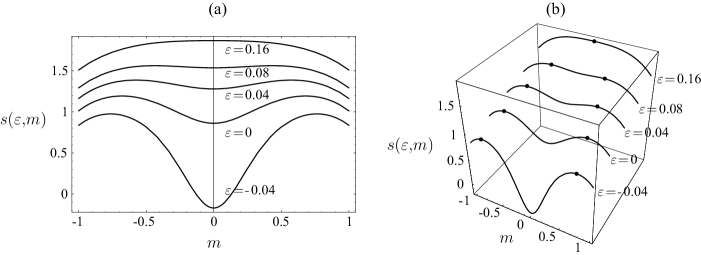
Figure 1: (a) Entropy as a function of the mean magnetization $m$ for different values of the mean energy $\varepsilon$. (b) 3D view of $s(\varepsilon,m)$. The black dots show the location of the equilibrium values of $m$ in the microcanonical ensemble for each value of $\varepsilon$ (see the text for explanation).

The entropy density $s(\varepsilon,m)$ of the mean-field $\phi^{4}$ model as a function of its mean energy $\varepsilon$ and mean magnetization $m$ is shown in Fig. 1. In Fig. 1(a), we have plotted the graph of $s(\varepsilon,m)$ as a function of $m$ for four different values of $\varepsilon$: one above the critical value $\varepsilon_{c}\approx 0.132$ and three below. To get a better idea of the shape of $s(\varepsilon,m)$ as a two-dimensional function, we also report in Fig. 1(b) the curves of Fig. 1(a) stacked along the $\varepsilon$ direction. The data shown in both of these plots are those obtained via the large deviation method, i.e., via the maximization problem displayed in (30). It should be noted that this maximization problem cannot be solved analytically because the free energy $\tilde{\varphi}_{m,v}(\lambda_{m},\lambda_{v})$, which intervenes in the derivation of the macrostate entropy function $\tilde{s}_{m,v}(m,v)$, involves a quartic integral; see Eq. (21). Nevertheless, this integral, like all the other quantities and optimization problems involved in the calculation of $s(\varepsilon,m)$, can easily be handled numerically with the end result that $s(\varepsilon,m)$ can easily be computed numerically to any desired precision. The specific results that we present in Fig. 1 were obtained with Mathematica using the default 16-digit working precision. The resulting numerical error is smaller than the tickness of the curves reported in Fig. 1.

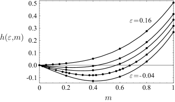
Figure 2: Effective magnetic field calculated using Rugh’s method ($\bullet$) and the large deviation method (full line). The values of $\varepsilon$ are from top to bottom $\varepsilon=0.16,0.08,0.04,0$ and $-0.04$. In this figure and in the next one the error associated with the results of the molecular dynamics simulations is smaller than the filled dots.

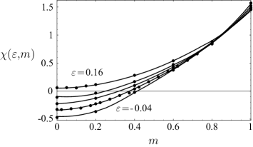
Figure 3: Magnetic susceptibility calculated using Rugh’s method ($\bullet$) and the large deviation method (full line).

The comparison of the large deviation method with Rugh’s method is reported in Figs. 2 and 3. Figure 2 shows the results of the calculation of the effective magnetic field $h(\varepsilon,m)$ using the large deviation method (full line) and Rugh’s method (filled dots). Because $s(\varepsilon,m)$ is an even function of $m$, we show $h(\varepsilon,m)$ only for $m>0$. In the former method, $h(\varepsilon,m)$ is calculated from its thermodynamic-limit definition

$$h(\varepsilon,m)=-T(\varepsilon,m)\frac{\partial s(\varepsilon,m)}{\partial m},$$ (53)

using the form of $s(\varepsilon,m)$ shown in Fig. 1. In the latter method, the same field is calculated using Eq. (43) or Eq. (48). As mentioned earlier, these two equations are expected to yield comparable results so long as the molecular dynamics simulations are performed for large-enough systems. In our case, $N=10^{2}$ particles were used, and we found no appreciable differences between the fields obtained with Eqs. (43) and (48). From Fig. 2, we see that there is a perfect agreement between the field $h(\varepsilon,m)$ obtained from the large deviation approach and the same field obtained from Rugh’s approach. We thus conclude that the two approaches agree on the calculation of $s(\varepsilon,m)$, up to a constant which can easily be determined. The two approaches perfectly agree also for the calculation of the magnetic susceptibility at constant energy; see Fig. 3.

Having shown that the large deviation approach for calculating $s(\varepsilon,m)$ gives the same results as those obtained with Rugh’s approach, we now come to the discussion of the nonequivalence of the microcanonical and canonical ensembles in relation to the nonconcavity of $s(\varepsilon,m)$. A first hint to the effect that the two ensembles are nonequivalent is provided by the fact that the effective field $h(\varepsilon,m)$ can be negative for positive values of $m$ when $\varepsilon<\varepsilon_{c}$, as can be seen from Fig. 2. In the canonical ensemble, it can be shown that the equilibrium magnetization of the mean-field $\phi^{4}$ model can only be negative when the canonically-imposed field $h$ is negative, and can only be positive when $h$ is positive. In other words, in the canonical ensemble, the magnetization of the $\phi^{4}$ model is always in the direction of the field. In the microcanonical ensemble, we see that this is not always the case: $h(\varepsilon,m)$ and $m$ can have opposite signs, so that this ensemble must be nonequivalent with the canonical ensemble.

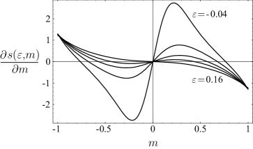
Figure 4: $m$-derivative of the entropy function shown in Fig. 1(a).

To understand how this peculiarity of the $\phi^{4}$ model arises out of the nonconcavity of $s(\varepsilon,m)$, we only have to analyze the definition of $h(\varepsilon,m)$, given by Eq. (53). There $T(\varepsilon,m)$ is always positive, since it is directly proportional to the kinetic energy, so that the sign of $h(\varepsilon,m)$ is always the opposite of the sign of $\partial s(\varepsilon,m)/\partial m$. Therefore, in order for $h(\varepsilon,m)$ to be negative for $m>0$, we must have $\partial s(\varepsilon,m)/\partial m>0$ for $m>0$. This, as can be seen by comparing Figs. 1(a), 2 and 4, can only happen if $s(\varepsilon,m)$ is nonconcave, i.e., if the graph of $s(\varepsilon,m)$ has a bimodal or “double-bump” shape as a function of the magnetization. When $s(\varepsilon,m)$ is concave or unimodal, as is the case for $\varepsilon=0.16$, then $\partial s(\varepsilon,m)/\partial m$ is necessarily negative when $m>0$ (Fig. 4), which implies that $h(\varepsilon,m)$ is necessarily positive when $m>0$ (Fig. 2), in agreement with what is seen in the canonical ensemble.

Another consequence of the nonconcavity of $s(\varepsilon,m)$ is that the magnetic susceptibility $\chi(\varepsilon,m)$, calculated microcanonically at fixed values of $\varepsilon$ and $m$, can be negative for certain values of $m$ and $\varepsilon$; see Fig. 3. This, alone, is a sure sign that the microcanonical and canonical ensembles are nonequivalent, for we know that the magnetic susceptibility is always positive in the canonical ensemble. Indeed, we know that by increasing the magnetic field $h$ while keeping the inverse temperature $\beta$ constant, the equilibrium magnetization $m(\beta,h)$ of the canonical ensemble can only increase, which means that

$$\chi(\beta,h)=\frac{\partial m(\beta,h)}{\partial h}\geq 0.$$ (54)

(See the Appendix for a general proof of this result.) In the microcanonical ensemble, the role of $h$ and $m$ are reversed: what is varied is $m$ not $h$, and the proper magnetic susceptibility to consider in this ensemble, defined as

$$\chi(\varepsilon,m)=\left(\frac{\partial h(\varepsilon,m)}{\partial m}\right)^{-1}=\left(\frac{\partial s}{\partial\varepsilon}\right)^{2}\left(\frac{\partial^{2}s}{\partial m\partial\varepsilon}\frac{\partial s}{\partial m}-\frac{\partial s}{\partial\varepsilon}\frac{\partial^{2}s}{\partial m^{2}}\right)^{-1},$$ (55)

can be negative, as demonstrated in Fig. 3. Physically, this means that, in the microcanonical ensemble, an increase in $m$ can lead to a decrease of the microcanonical field $h(\varepsilon,m)$. This, as we have already mentioned, is related to the fact that $s(\varepsilon,m)$ is nonconcave as a function of $m$; however, it is important to note that $\chi(\varepsilon,m)$ does not become negative exactly when $s(\varepsilon,m)$ becomes nonconcave. Indeed, the local convexity properties of $s(\varepsilon,m)$ are determined by the eigenvalues of the Hessian matrix

$$\left(\begin{array}[]{cc}\partial^{2}s/\partial m^{2}&\partial^{2}s/\partial m\partial\varepsilon\\ \partial^{2}s/\partial\varepsilon\partial m&\partial^{2}s/\partial\varepsilon^{2}\end{array}\right)~{},$$ (56)

whose characteristic equation is

$$x^{2}-\left[\frac{\partial^{2}s}{\partial m^{2}}+\frac{\partial^{2}s}{\partial\varepsilon^{2}}\right]x+\left[\frac{\partial^{2}s}{\partial m^{2}}\frac{\partial^{2}s}{\partial\varepsilon^{2}}-\left(\frac{\partial^{2}s}{\partial m\partial\varepsilon}\right)^{2}\right]=0~{}.$$ (57)

The sign of the eigenvalues of the Hessian changes when either the sign of the first-order term or of the zeroth-order term of the characteristic equation changes. This occurs on two lines in the $(\varepsilon,m)$ plane, which can either intersect at one point on the line where the susceptibility given in Eq. (55) changes sign, or not intersect at all. In either case, the change in the local convexity properties of $s(\varepsilon,m)$ and in the sign of $\chi(\varepsilon,m)$ does not happen generically at the same value of $m$ for a given value of $\varepsilon$. This is also seen by comparing Figs. 3 and 4.

To close our discussion of the mean-field $\phi^{4}$ model, we now comment on the thermodynamic properties of this model obtained from the microcanonical ensemble in which only the energy is fixed. In this ensemble, the relevant entropy function to consider is the function $s(\varepsilon)$ defined in Eq. (4). From the knowledge of $s(\varepsilon,m)$, we can derive $s(\varepsilon)$ by using the following contraction formula Ellis et al. (2000, 2004):

$$s(\varepsilon)=\sup_{m}s(\varepsilon,m).$$ (58)

Figure 1(b) shows the positions of the maxima of $s(\varepsilon,m)$, which represent physically the equilibrium values of the magnetization in the microcanonical ensemble with fixed energy $N\varepsilon$. We see from this figure that $s(\varepsilon,m)$ has only one maximum located at $m=0$ when it is concave as a function of $m$. This happens when $\varepsilon\geq\varepsilon_{c}$, so that $s(\varepsilon)=s(\varepsilon,m=0)$ for all $\varepsilon\geq\varepsilon_{c}$. Below $\varepsilon_{c}$, the single maximum of $s(\varepsilon,m)$ splits in a continuous way into two symmetric maxima. The continuous character of the splitting can be deduced from the fact that the phase transition of the model, seen in the canonical ensemble having $\beta$ as its only parameter, is known to be of second order Dauxois et al. (2003). This implies that the phase transition seen in the microcanonical ensemble as a function of $\varepsilon$ is also second-order, i.e., continuous. This must be so because a second-order phase transition in the canonical ensemble implies that the canonical and microcanonical ensembles are fully equivalent, since $s(\varepsilon)$ in this case is concave and has no affine parts, i.e., no straight (linear) lines in its graph Touchette (2003); Ellis et al. (2004); Touchette (2006); Costeniuc et al. (2006a). These two features of $s(\varepsilon)$ are somewhat difficult to see from Fig. 1; however, they are confirmed by the theory of nonconcave entropies. The fact indeed is that if $s(\varepsilon)$ was nonconcave as a function of $\varepsilon$, then the phase transition of the model would be first-order as a function of the temperature rather than second-order Touchette (2003, 2006). The same applies if $s(\varepsilon)$ was affine: in this case, the phase transition in the canonical ensemble would also be first-order Touchette (2003, 2006), which is not what is reported by Dauxois et al. Dauxois et al. (2003).

The relationship between nonconcave entropies and first-order phase transitions is fully general, and can be applied to $s(\varepsilon,m)$ to conclude that the mean-field $\phi^{4}$ model displays, in the canonical ensemble with temperature $T$ and magnetic field $h$, a first-order, field-driven phase transition when $T<T_{c}=2\varepsilon_{c}$. The phase transition, in this case, is driven by the magnetic field $h$ because the entropy $s(\varepsilon,m)$ is nonconcave as a function of the magnetization, the variable conjugated to $h$. Moreover, since $h$ is basically the derivative of $s(\varepsilon,m)$, it should be clear from the symmetric, bimodal shape of $s(\varepsilon,m)$, seen again when $\varepsilon<\varepsilon_{c}$, that the critical field of the phase transition is $h_{c}=0$. Physically, this means that if we set the temperature $T$ to be below $T_{c}$, then the equilibrium magnetization $m(T,h)$ of the canonical ensemble jumps from a negative, non-zero value to a positive, non-zero value as $h$ varies from $0^{-}$ to $0^{+}$. The “spontaneous” values of $m(T,h)$ found for $h=0^{-}$ and $h=0^{+}$ are nothing but the two values of $m$ at which $s(\varepsilon,m)$ if maximum when $\varepsilon<\varepsilon_{c}$.

VI Conclusion

The entropy of long-range systems can be concave as a function of the energy alone, and yet be nonconcave as a function of the energy and other invariant quantities. This was illustrated here for the mean-field $\phi^{4}$ model: its entropy is concave as a function of the energy, but is nonconcave as a function of the energy and magnetization. This property of the entropy leads, as we have shown, to a fundamental difference between the thermodynamic properties of the model found in the microcanonical ensemble as a function of the energy and magnetization, and those found in the canonical ensemble as a function of the temperature and magnetic field. On the one hand, we have shown that the (effective) magnetic field of the microcanonical ensemble can have a sign opposite to that of the magnetization. In the canonical ensemble, this never happens, as the equilibrium magnetization in this ensemble is always in the direction of the applied magnetic field. On the other hand, we showed that the magnetic susceptibility at constant temperature, calculated microcanonically as a function of the energy and magnetization, can be negative, whereas it is always positive in the canonical ensemble. Because of these two differences, we say that the microcanonical and canonical ensembles are nonequivalent.

There is a further consequence of the nonconcavity of the entropy that we have discussed, namely that the mean-field $\phi^{4}$ model displays a first-order phase transition driven by the magnetic field in the canonical ensemble. This phase transition is directly related to the fact that the entropy of the model is nonconcave as a function of the magnetization—the quantity conjugated to the magnetic field—for certain values of the energy. Thus, in addition to display a second-order phase transition driven by the temperature (or the energy), the mean-field $\phi^{4}$ model displays a first-order phase transition driven by the magnetic field. The situation, as such, is similar to the two-dimensional Ising model, which also displays a second-order phase transition in temperature but a first-order phase transition in the magnetic field. There is, however, a fundamental difference between the Ising model and the mean-field $\phi^{4}$ model. Being a short-range interaction model, the Ising model has an entropy which is necessarily concave as a function of its energy and magnetization Ruelle (1969). The first-order, field-driven phase transition of this model is thus not related to a nonconcavity of the entropy; it appears, in fact, because the entropy, when plotted as a function of the magnetization, has affine parts in the form of “plateaus.” For more details on this point, we refer the reader to Sec. 11 of Ref. Ellis (1995) and the references cited therein.

Our last words of this paper will go to a technical remark about a possible way to compute the entropy $s(\varepsilon,m)$ using Legendre transforms. We mentioned in Sec. II that because $s(\varepsilon,m)$ is nonconcave, it cannot be calculated as the Legendre transform of the energy function $\varphi(\beta,\eta)$ or, equivalently, $\varphi(\beta,h)$, which is the free energy associated with the partition function shown in (9). However, there is a subtle workaround to this problem. Indeed, although $s(\varepsilon,m)$ is nonconcave as a function of $m$, it is concave in $\varepsilon$ for all $m$. This suggests that the projections of $s(\varepsilon,m)$ along $\varepsilon$ can be calculated by taking the Legendre transform of a free energy function, which, unconventionally, is a function of the inverse temperature and the magnetization. The construction of this Legendre transform, which follow from the theory of Ellis et al. Ellis et al. (2000), is outlined in Appendix B.

Appendix A Proof of the positivity of $\chi(\beta,h)$

The equilibrium magnetization $m(\beta,h)$, calculated in the canonical ensemble as a function of the inverse temperature $\beta$ and magnetic field $h$, can be deduced from the equation

$$m(\beta,h)=-\frac{1}{\beta}\frac{\partial\varphi(\beta,h)}{\partial h},$$ (59)

where $\varphi(\beta,h)$ is the canonical free energy function associated with the partition function shown in (9). With this equation, the definition of the magnetic susceptibility $\chi(\beta,h)$ in the canonical ensemble can be rewritten as

$$\chi(\beta,h)=-\frac{1}{\beta}\frac{\partial^{2}\varphi(\beta,h)}{\partial h^{2}}.$$ (60)

At this point, we note that $\varphi(\beta,h)$ is an always convex function of $\beta$ and $h$, so that

$$\frac{\partial^{2}\varphi(\beta,h)}{\partial h^{2}}\leq 0$$ (61)

for all $\beta$ and $h$. Consequently, $\chi(\beta,h)\geq 0$ for all values of $\beta>0$ and $h$, as claimed.

Appendix B Mixed canonical-microcanonical ensemble

Define the partition function

$$Z(\beta,m)=\int_{\Gamma}e^{-\beta H(x)}\delta(m(x)-m)dx$$ (62)

and its associated free energy

$$\varphi(\beta,m)=-\lim_{N\rightarrow\infty}\frac{1}{N}\ln Z(\beta,m).$$ (63)

Then

$$s(\varepsilon,m)=\beta\varepsilon-\varphi(\beta,m),$$ (64)

where the value of $\beta$ is set by solving

$$\frac{\partial\varphi(\beta,m)}{\partial\beta}=\varepsilon.$$ (65)

The last two equations define the Legendre transform that takes $\varphi(\beta,m)$ to $s(\varepsilon,m)$. It is a valid Legendre transform for the mean-field $\phi^{4}$ model because $s(\varepsilon,m)$ is concave as a function of $\varepsilon$ for all values of $m$ for this model; see Fig. 1. Following Ellis et al. Ellis et al. (2000), $Z(\beta,m)$ and $\varphi(\beta,m)$ are to be interpreted, respectively, as the partition function and free energy function of a mixed canonical-microcanonical ensemble in which the energy is treated in a canonical way, while the magnetization is treated in a microcanonical way. The reader is referred to Ref. Ellis et al. (2000) for more details on the idea of mixed ensembles.

References

- Gross (1997) D. H. E. Gross, Phys. Rep. 279, 119 (1997).
- Gross (2001) D. H. E. Gross, Microcanonical Thermodynamics: Phase Transitions in “Small” Systems, vol. 66 of Lecture Notes in Physics (World Scientific, Singapore, 2001).
- Eyink and Spohn (1993) G. L. Eyink and H. Spohn, J. Stat. Phys. 70, 833 (1993).
- Ellis et al. (2000) R. S. Ellis, K. Haven, and B. Turkington, J. Stat. Phys. 101, 999 (2000).
- Dauxois et al. (2002) T. Dauxois, S. Ruffo, E. Arimondo, and M. Wilkens, in Dynamics and Thermodynamics of Systems with Long Range Interactions, edited by T. Dauxois, S. Ruffo, E. Arimondo, and M. Wilkens (Springer, New York, 2002), vol. 602 of Lecture Notes in Physics.
- Touchette et al. (2004) H. Touchette, R. S. Ellis, and B. Turkington, Physica A 340, 138 (2004).
- Ispolatov and Cohen (2000) I. Ispolatov and E. G. D. Cohen, Physica A 295, 475 (2000).
- Barré et al. (2001) J. Barré, D. Mukamel, and S. Ruffo, Phys. Rev. Lett. 87, 030601 (2001).
- Ellis et al. (2004) R. S. Ellis, H. Touchette, and B. Turkington, Physica A 335, 518 (2004).
- Costeniuc et al. (2005a) M. Costeniuc, R. S. Ellis, and H. Touchette, J. Math. Phys. 46, 063301 (2005a).
- Barré et al. (2005) J. Barré, F. Bouchet, T. Dauxois, and S. Ruffo, J. Stat. Phys. 119, 677 (2005).
- Hahn and Kastner (2006) I. Hahn and M. Kastner, Eur. Phys. J. B 50, 311 (2006).
- Costeniuc et al. (2005b) M. Costeniuc, R. S. Ellis, H. Touchette, and B. Turkington, J. Stat. Phys. 119, 1283 (2005b).
- Costeniuc et al. (2006a) M. Costeniuc, R. S. Ellis, H. Touchette, and B. Turkington, Phys. Rev. E 73, 026105 (2006a).
- Touchette and Beck (2006) H. Touchette and C. Beck, J. Stat. Phys. 125, 455 (2006).
- Costeniuc et al. (2006b) M. Costeniuc, R. S. Ellis, and H. Touchette, Phys. Rev. E 74, 010105 (2006b).
- Lynden-Bell and Wood (1968) D. Lynden-Bell and R. Wood, Mon. Notic. Roy. Astron. Soc. 138, 495 (1968).
- Thirring (1970) W. Thirring, Z. Physik 235, 339 (1970).
- Chavanis (2002) P.-H. Chavanis, Phys. Rev. E 65, 056123 (2002).
- Chavanis and Ispolatov (2002) P.-H. Chavanis and I. Ispolatov, Phys. Rev. E 66, 036109 (2002).
- Smith and O’Neil (1990) R. A. Smith and T. M. O’Neil, Phys. Fluids B 2, 2961 (1990).
- Kiessling and Lebowitz (1997) M. K.-H. Kiessling and J. Lebowitz, Lett. Math. Phys. 42, 43 (1997).
- Ellis et al. (2002) R. S. Ellis, K. Haven, and B. Turkington, Nonlinearity 15, 239 (2002).
- Lynden-Bell (1999) D. Lynden-Bell, Physica A 263, 293 (1999).
- Touchette (2003) H. Touchette, Ph.D. thesis, McGill University (2003).
- Hahn and Kastner (2005) I. Hahn and M. Kastner, Phys. Rev. E 72, 056134 (2005).
- Rugh (1998) H. H. Rugh, J. Phys. A: Math. Gen. 31, 7761 (1998).
- Rugh (2001) H. H. Rugh, Phys. Rev. E 64, 055101 (2001).
- Desai and Zwanzig (1978) R. Desai and R. Zwanzig, J. Stat. Phys. 19, 1 (1978).
- Dauxois et al. (2003) T. Dauxois, S. Lepri, and S. Ruffo, Commun. Nonlinear Sc. Num. Simul. 8, 375 (2003).
- Campa and Ruffo (2006) A. Campa and S. Ruffo, Physica A 369, 517 (2006).
- Ellis (1985) R. S. Ellis, Entropy, Large Deviations, and Statistical Mechanics (Springer-Verlag, New York, 1985).
- Ellis (1999) R. S. Ellis, Physica D 133, 106 (1999).
- Touchette (2006) H. Touchette, Physica A 359, 375 (2006).
- Ruelle (1969) D. Ruelle, Statistical Mechanics: Rigorous Results (W.A. Benjamin, Reading, 1969).
- Ellis (1995) R. S. Ellis, Scand. Actuarial J. 1, 97 (1995).