Mixtures of Bose gases under rotation

Abstract

We examine the rotational properties of a mixture of two Bose gases. Considering the limit of weak interactions between the atoms, we investigate the behavior of the system under a fixed angular momentum. We demonstrate a number of exact results in this many-body system.

One of the many interesting aspects of the field of cold atoms is that one may create mixtures of different species. The equilibrium density distribution of the atoms is an interesting problem by itself, since the different components may coexist, or separate, depending on the value of the coupling constants between the atoms of the same and of the different species. If this system rotates, the problem becomes even more interesting. In this case, the state of lowest energy may involve rotation of either one of the components, or rotation of all the components. Actually, the first vortex state in cold gases of atoms was observed experimentally in a two-component system Cornell1 , following the theoretical suggestion of Ref. Holland . More recently, vortices have also been created and observed in spinor Bose-Einstein condensates Ketterle ; Cornell2 . Theoretically, there have been several studies of this problem Ho ; Ueda1 ; Ueda2 , mostly in the case where the number of vortices is relatively large. Kasamatsu, Tsubota, and Ueda have also given a review of the work that has been done on this problem Uedareview .

In this Letter, we consider a rotating two-component Bose gas in the limit of weak interactions and slow rotation, where the number of vortices is of order unity. Surprisingly, a number of exact analytical results exist for the energy of this system. The corresponding many-body wavefunction also has a relatively simple structure.

We assume equal masses $M$ for the two components, and a harmonic trapping potential $V_{t}=M(\omega^{2}\rho^{2}+\omega_{z}^{2}z^{2})/2$, with $\rho^{2}=x^{2}+y^{2}$. The trapping frequency $\omega_{z}$ along the axis of rotation is assumed to be much higher than $\omega$. In addition, we consider weak atom-atom interactions, much smaller than the oscillator energy $\hbar\omega$, and work within the subspace of states of the lowest Landau level. The motion of the atoms is thus frozen along the axis of rotation and our problem becomes quasi-two-dimensional Ben . The relevant eigenstates are $\Phi_{m}(\rho,\theta)\varphi_{0}(z)$, where $\Phi_{m}(\rho,\theta)$ are the lowest-Landau-level eigenfunctions of the two-dimensional oscillator with angular momentum $m\hbar$, and $\varphi_{0}(z)$ is the lowest harmonic oscillator eigenstate along the $z$ axis.

The assumption of weak interactions also excludes the possibility of phase separation in the absence of rotation phasesep , since the atoms of both species reside in the lowest state $\Phi_{0,0}({\bf r})=\Phi_{0}(\rho,\theta)\varphi_{0}(z)$, while the depletion of the condensate due to the interaction may be treated perturbatively.

We label the two (distinguishable) components of the gas as $A$ and $B$. In what follows the atom-atom interaction is assumed to be a contact potential of equal scattering lengths for collisions between the same species and the different ones, $a_{AA}=a_{BB}=a_{AB}=a$. The interaction energy is measured in units of $v_{0}=U_{0}\int|\Phi_{0,0}({\bf r})|^{4}\,d^{3}r=(2/\pi)^{1/2}\hbar\omega a/a_{z}$, where $U_{0}=4\pi\hbar^{2}a/M$, and $a_{0}=(\hbar/M\omega)^{1/2}$, $a_{z}=(\hbar/M\omega_{z})^{1/2}$ are the oscillator lengths on the plane of rotation and perpendicular to it.

If $N_{A}$ and $N_{B}$ denote the number of atoms in each component, we examine the behavior of this system for a fixed amount of $L$ units of angular momentum, with $0\leq L\leq N_{\rm max}$, where $N_{\rm max}={\rm max}(N_{A},N_{B})$. We use both numerical diagonalization of the many-body Hamiltonian for small systems, as well as the mean-field approximation. Remarkably, as we explain in detail below, there is a number of exact results in this range of angular momenta.

More specifically, when $0\leq L\leq N_{\rm min}$, where $N_{\rm min}={\rm min}(N_{A},N_{B})$, using exact diagonalization of the many-body Hamiltonian, we find that the interaction energy of the lowest-energy state has a parabolic dependence on $L$ in this range,

$${\cal E}_{0}(L)/v_{0}=\frac{1}{2}N(N-1)-\frac{1}{2}NL+\frac{1}{4}L(L-1),$$ (1)

with $N=N_{A}+N_{B}$. In addition, the lowest-energy state consists only of the single-particle states of the harmonic oscillator with $m=0$ and $m=1$. The occupancy of the $m=1$ state of each component is given by

$$(N_{A})_{m=1} = L\frac{N_{B}-L+1}{N-2L+2},$$ (2)

$$(N_{B})_{m=1} = L\frac{N_{A}-L+1}{N-2L+2},$$ (3)

while $(N_{A})_{m=0}=N_{A}-(N_{A})_{m=1}$, and $(N_{B})_{m=0}=N_{B}-(N_{B})_{m=1}$.

Figure 1: The interaction energy that results from numerical diagonalization of the Hamiltonian of a mixture of two Bose gases, with $N_{A}=4$ and $N_{B}=12$ (lower curve, marked by “+”), as well as $N_{A}=16$, and $N_{B}=0$ (higher curve, marked by “x”), as function of the angular momentum $L$, for $0\leq L\leq 12$.

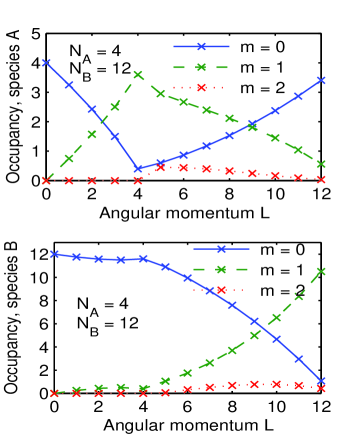
Figure 2: The occupancy of the single-particle states with $m=0,1$ and 2, as function of the angular momentum $0\leq L\leq 12$, that results from numerical diagonalization of the Hamiltonian of a mixture of two Bose gases, with $N_{A}=4$ and $N_{B}=12$. The upper panel refers to species $A$, and the lower one to species $B$.

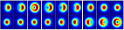
Figure 3: The conditional probability distribution of a mixture of two Bose gases, with $N_{A}=4$ (higher row), and $N_{B}=12$ (lower row). Each graph extends between $-2.4a_{0}$ and $2.4a_{0}$. The reference point is located at $(x,y)=(a_{0},0)$ in the higher graph. The angular momentum $L$ increases from left to right, $L=2,3,4(=N_{A}),5,6,8,10,11$, and $12(=N_{B})$.

As $L$ becomes larger than $N_{\rm min}$, there is a phase transition. For $N_{\rm min}\leq L\leq N_{\rm max}$, the single-particle states that constitute the many-body state are no longer only the ones with $m=0$ and $m=1$ (as in the case $0\leq L\leq N_{\rm min}$), and in addition the interaction energy varies linearly with $L$,

$${\cal E}_{0}(L)/v_{0}=\frac{1}{2}N(N-1)-\frac{1}{4}N_{\rm min}N$$

$$-\frac{1}{4}NL+\frac{1}{4}N_{\rm min}(N_{\rm min}-1).$$ (4)

The lower curve in Fig. 1 shows the interaction energy of a system with $N_{A}=4$ and $N_{B}=12$, for $0\leq L\leq 12$. For $0\leq L\leq 4$ the energy is parabolic, and for $4\leq L\leq 12$, it is linear. These are exact results, within numerical accuracy. The higher curve is the interaction energy of a single-component system of $N=16$ atoms. It is known that in this case, the interaction energy is exactly linear for $2\leq L\leq N=16$ Bertsch . This line is parallel to the line which gives the interaction energy of the system with $N_{A}=4$ and $N_{B}=12$ for $N_{A}=4\leq L\leq N_{B}=12$. Figure 2 shows the occupancy of the single-particle states, that result from the numerical diagonalization of the Hamiltonian.

The physical picture that emerges from these calculations is intriguing: as $L$ increases, a vortex state enters the component with the smaller population from infinity and ends up at the center of the trap when $L=N_{\rm min}$. In addition, another vortex state enters the component with the larger population from the opposite side of the trap, reaching a minimum distance from the center of the trap for $L\approx N_{A}/2$ (this estimate is valid if $1\ll N_{A}\ll N_{B}$), and then returns to infinity when $L=N_{\rm min}$. This minimum distance is $\approx 2(N_{B}/N_{A})a_{0}$. For $N_{\rm min}\leq L\leq N_{\rm max}$, the vortex in the cloud with the smaller population (that is located at the center of the trap when $L=N_{\rm min}$) moves outwards, ending up at infinity when $L=N_{\rm max}$, while a vortex in the other component moves inwards again, ending up at the center of the trap when $L=N_{\rm max}$. Figure 3 shows clearly these effects via the conditional probability distributions, for $N_{A}=4$, and $N_{B}=12$. We note that in the range $0<L<N_{A}=4$, the (distant) vortex in the large component (lower row, species $B$) is too far away from the center of the cloud to be visible, because of the exponential drop of the density. The plots in Fig. 3 (and Fig. 5) are not very sensitive to the total number of atoms $N=N_{A}+N_{B}$, and resemble the behavior of the system in the thermodynamic limit of large $N$.

In the case of equal populations, $N_{A}=N_{B}$, the parabolic expression for the interaction energy, Eq. (1), holds all the way between $0\leq L\leq N_{A}=N_{B}$. Figure 4 shows the interaction energy and Fig. 5 the occupancies of the single-particle states, which vary linearly with $L$. The corresponding physical picture is quite different in this case, as shown in Fig.  6. The system is now symmetric with respect to the two components, and a vortex state enters each of the components (from opposite sides). These vortices reach a minimum distance from the center of the trap equal to $a_{0}$, when $L=N_{A}=N_{B}$.

Figure 4: The interaction energy that results from numerical diagonalization of the Hamiltonian of a mixture of two Bose gases, with $N_{A}=N_{B}=8$, as function of the angular momentum $L$, for $0\leq L\leq 8$.

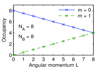
Figure 5: The occupancy of the single-particle states with $m=0$ and $m=1$, as function of the angular momentum $0\leq L\leq 8$, that results from numerical diagonalization of the Hamiltonian of a mixture of two Bose gases, with $N_{A}=N_{B}=8$.

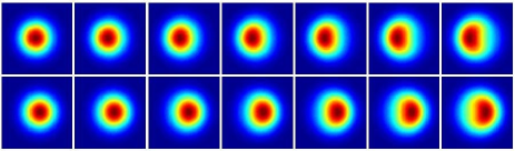
Figure 6: The conditional probability distribution of a mixture of two Bose gases, with $N_{A}=N_{B}=8$. The two rows refer to the two different species. Each graph extends between $-2.4a_{0}$ and $2.4a_{0}$. The reference point is located at $(x,y)=(a_{0},0)$ in the lower graph. The angular momentum $L$ increases from left to right, $L=2,3,\dots,8$.

The simplicity of the system that we have studied allows one to get some relatively simple analytical results, which we present below. As we saw earlier, when $L=N_{A}$ or $L=N_{B}$, there is a unit vortex state in species $A$ or $B$, while the other species is in the lowest oscillator state with $m=0$. Since (at least to leading order and next to leading order) only the states with $m=0$ and $m=1$ are occupied, the Fock states are of the general form (if, for example, $L=N_{B}$)

$$|n\rangle=|0^{N_{A}-n},1^{n}\rangle\bigotimes|0^{n},1^{N_{B}-n}\rangle.$$ (5)

Expressing the eigenstates of the interaction $V$ as $|\Phi\rangle=\sum_{n}(-1)^{n}f_{n}|n\rangle$, the eigenvalue equation takes the form

$$V_{n,n}f_{n}-V_{n,n-1}f_{n-1}-V_{n,n+1}f_{n+1}={\cal E}f_{n},$$ (6)

where $V_{n,m}$ are the matrix elements of the interaction between the above states. Remarkably, if $N_{A}=N_{B}=N/2$, then

$$V_{n,n}-V_{n,n-1}-V_{n,n+1}=5N(N-2)v_{0}/16,$$ (7)

which implies that in this case, the lowest eigenenergy is ${\cal E}_{0}=5N(N-2)v_{0}/16$, in agreement with Eq. (1). The corresponding eigenfunction is simply $|\Phi_{0}\rangle=\sum_{n}(-1)^{n}|n\rangle$.

In the case $N_{A}\neq N_{B}$, with, e.g., $L=N_{B}$, $n$ is of order unity, and therefore the interaction may be written as

$$V/v_{0}=\frac{1}{2}N_{A}(N_{A}-1)+\frac{1}{4}N_{B}(N_{B}-1)+\frac{1}{2}N_{A}N_{B}+$$

$$+\frac{1}{2}(N_{A}+N_{B}){\hat{a}}_{0}^{\dagger}{\hat{a}}_{0}+\frac{1}{2}\sqrt{N_{A}N_{B}}({\hat{a}}_{0}{\hat{b}}_{1}^{\dagger}+{\hat{a}}_{0}^{\dagger}{\hat{b}}_{1}),$$ (8)

where ${\hat{a}}_{m}({\hat{a}}_{m}^{\dagger})$ and ${\hat{b}}_{m}({\hat{b}}_{m}^{\dagger})$ are annihilation (creation) operators of the species $A$ and $B$ with angular momentum $m\hbar$. The above expression for $V$ can be diagonalized with a Bogoliubov transformation,

$$V/v_{0}=\frac{1}{4}|N_{A}-N_{B}|(2{\hat{\alpha}}^{\dagger}{\hat{\alpha}}+1)+\frac{1}{4}N_{A}(2N_{A}-3)+$$

$$+\frac{1}{4}N_{B}(N_{B}-2)+\frac{1}{2}N_{A}N_{B},$$ (9)

where ${\hat{\alpha}}^{\dagger}{\hat{\alpha}}$ is a number operator. When $N_{A}=N_{B}=N/2$, the lowest eigenenergy is $5N(N-2)/16$, in agreement with Eq. (1). When $N_{A}\neq N_{B}$, the lowest eigenenergy is

$${\cal E}_{0}/v_{0}=\frac{1}{4}|N_{A}-N_{B}|+\frac{1}{4}N_{A}(2N_{A}-3)+$$

$$+\frac{1}{4}N_{B}(N_{B}-2)+\frac{1}{2}N_{A}N_{B}.$$ (10)

The above expression agrees exactly with Eq. (1) when $N_{A}<N_{B}=L$, and to leading order in $N$ when $N_{A}>N_{B}=L$.

In addition, according to Eq. (9), the excitation energies are equally spaced, separated by $|N_{A}-N_{B}|v_{0}/2+{\cal O}(v_{0})$. Therefore, one very important difference between the case $N_{A}=N_{B}$ and $N_{A}\neq N_{B}$ is that in the first case there are low-lying excited states, with an energy separation of order $v_{0}$, while in the second [where in general $N_{A}-N_{B}\sim{\cal O}(N)$], the low-lying excited states are separated from the lowest state by an energy of order $Nv_{0}$.

Let us now turn to the mean-field description of this system, for $0\leq L\leq N_{\rm min}$. We consider the following order parameters for the two species (restricting ourselves to the states with $m=0$ and $m=1$ only),

$$\Psi_{A}=(c_{0}\Phi_{0}+c_{1}\Phi_{1})\varphi_{0}(z),\\ \Psi_{B}=(d_{0}\Phi_{0}+d_{1}\Phi_{1})\varphi_{0}(z),$$

where $c_{0}$, $c_{1}$, $d_{0}$, $d_{1}$ are variational parameters. Given the order parameters, the many-body state is $\Phi_{\rm MF}=\prod_{i=1}^{N_{A}}\Phi_{A}({\bf r}_{i})\prod_{j=1}^{N_{B}}\Phi_{B}({\bf r}_{j})$. The normalization for each species implies that $|c_{0}|^{2}+|c_{1}|^{2}=1$, and $|d_{0}|^{2}+|d_{1}|^{2}=1$, while the condition for the angular momentum gives $N_{A}|c_{1}|^{2}+N_{B}|d_{1}|^{2}=L$. The interaction energy is

$${\cal E}_{\rm MF} = \frac{1}{2}N_{A}(N_{A}-1)U_{0}\int|\Phi_{A}|^{4}\,d^{3}r+$$ (11)

$$+ \frac{1}{2}N_{B}(N_{B}-1)U_{0}\int|\Phi_{B}|^{4}\,d^{3}r+$$

$$+ N_{A}N_{B}U_{0}\int|\Phi_{A}|^{2}|\Phi_{B}|^{2}\,d^{3}r,$$

or, to leading order in $N$,

$$\frac{{\cal E}_{\rm MF}}{N^{2}v_{0}}=\frac{1}{2}\left(\frac{N_{A}}{N}\right)^{2}\left(|c_{0}|^{4}+\frac{1}{2}|c_{1}|^{4}+2|c_{0}|^{2}|c_{1}|^{2}\right)+$$

$$+\frac{1}{2}\left(\frac{N_{B}}{N}\right)^{2}\left(|d_{0}|^{4}+\frac{1}{2}|d_{1}|^{4}+2|d_{0}|^{2}|d_{1}|^{2}\right)+$$

$$+\frac{N_{A}N_{B}}{N^{2}}\left(|c_{0}|^{2}|d_{0}|^{2}+\frac{1}{2}|c_{0}|^{2}|d_{1}|^{2}+\frac{1}{2}|c_{1}|^{2}|d_{0}|^{2}+\right.$$

$$\left.+\frac{1}{2}|c_{1}|^{2}|d_{1}|^{2}-|c_{0}||c_{1}||d_{0}||d_{1}|\right),$$ (12)

where the phases of the variational coefficients have been chosen so as to minimize ${\cal E}_{\rm MF}$.

When $N_{A}=N_{B}$, then $|c_{0}|^{2}=|d_{0}|^{2}$, and also $|c_{1}|^{2}=|d_{1}|^{2}$, which implies that $|c_{1}|^{2}=|d_{1}|^{2}=L/N=l$. Therefore, one finds that ${\cal E}_{\rm MF}/N^{2}=(2-2l+{l^{2}})v_{0}/4$, in agreement (to leading order in $N$) with the result of exact diagonalization, Eq. (1). When $N_{A}\neq N_{B}$, minimization of the energy with respect to one of the four (free) variational parameters (the other three are then fixed by the three constraints) gives a result that agrees to leading order in $N$ with that of numerical diagonalization.

The fact that for $0\leq L\leq N_{\rm min}$ the lowest many-body state consists of only the $m=0$ and $m=1$ single-particle states is remarkable. To get some insight into this result, we consider the two coupled Gross-Pitaevskii equations, which describe the order parameters $\Psi_{A}$ and $\Psi_{B}$. If $\mu_{A}$ and $\mu_{B}$ is the chemical potential of each component, then

$$\left(-\frac{\hbar^{2}\nabla^{2}}{2M}+V_{t}+U_{0}|\Psi_{B}|^{2}\right)\Psi_{A}+U_{0}|\Psi_{A}|^{2}\Psi_{A} = \mu_{A}\Psi_{A},$$

$$\left(-\frac{\hbar^{2}\nabla^{2}}{2M}+V_{t}+U_{0}|\Psi_{A}|^{2}\right)\Psi_{B}+U_{0}|\Psi_{B}|^{2}\Psi_{B} = \mu_{B}\Psi_{B}.$$

For a large population imbalance, where, for example, $1\ll N_{A}\ll N_{B}$, for $0\leq L\leq N_{\rm min}=N_{A}$, most of the angular momentum is carried by the species $A$ (with the smaller population). As mentioned earlier, in the range $0\leq L\leq N_{\rm min}$, although there is also a vortex state in species $B$, this is far away from the center of the cloud. As a result, the order parameter of species $B$ is essentially the Gaussian state, with the corresponding density being $|\Psi_{B}(\rho,z)|^{2}\approx n_{B}(0,0)e^{-\rho^{2}/a_{0}^{2}-z^{2}/a_{z}^{2}}$, where $n_{B}(0,0)$ is the density of species $B$ at the center of the trap, i.e., at $\rho=0$ and $z=0$.

This component acts as an external potential on species $A$. Thus, the total “effective” potential acting on species $A$ is (expanding the function $e^{-\rho^{2}/a_{0}^{2}}$),

$$V_{\rm eff}(\rho,0)\approx\frac{M}{2}\omega^{2}\rho^{2}+U_{0}\,n_{B}(0,0)\left(1-\frac{\rho^{2}}{a_{0}^{2}}+\frac{\rho^{4}}{2a_{0}^{4}}\right),$$ (14)

for distances close to the center of the cloud. One may argue that in this self-consistent analysis, the quadratic term in the expansion changes the effective trap frequency, while the quartic term acts as an anharmonic potential. We argue that this anharmonic term is responsible for the fact that only the states with $m=0$ and $m=1$ are occupied Emil . Actually, this is more or less how Dalibard et al. investigated the problem of multiple quantization of vortex states Dalibard . In that case, it was an external laser beam that created an external, repulsive Gaussian potential, as opposed to the present problem, where this potential results from the interaction between the different components.

We acknowledge financial support from the European Community project ULTRA-1D (NMP4-CT-2003-505457), the Swedish Research Council, and the Swedish Foundation for Strategic Research.

References

(1) M. R. Matthews, B. P. Anderson, P. C. Haljan,
D. S. Hall, C. E. Wieman, and E. A. Cornell, Phys. Rev. Lett.
83, 2498 (1999).
(2) J. E. Williams and M. J. Holland, Nature
(London) 401, 568 (1999).
(3) A. E. Leanhardt, Y. Shin, D. Kielpinski,
D. E. Pritchard, and W. Ketterle, Phys. Rev. Lett. 90,
140403 (2003).
(4) V. Schweikhard, I. Coddington, P. Engels,
S. Tung, and E. A. Cornell, Phys. Rev. Lett. 93, 210403
(2004).
(5) E. J. Mueller and T.-L. Ho, Phys. Rev. Lett. 88,
180403 (2002).
(6) K. Kasamatsu, M. Tsubota, and M. Ueda
Phys. Rev. Lett. 91, 150406 (2003).
(7) K. Kasamatsu, M. Tsubota, and M. Ueda
Phys. Rev. A 71, 043611 (2005).
(8) K. Kasamatsu, M. Tsubota, and M. Ueda,
Int. J. of Mod. Phys. B, 19, 1835 (2005).
(9) B. Mottelson, Phys. Rev. Lett. 83, 2695 (1999).
(10) C. J. Pethick and H. Smith, Bose-Einstein
Condensation in Dilute Gases (Cambridge University Press,
Cambridge, 2002).
(11) See, e.g., G. F. Bertsch and T. Papenbrock,
Phys. Rev. Lett. 83, 5412 (1999), and references therein.
(12) See, e.g., A. L. Fetter, Phys. Rev. A 64,
063608 (2001); E. Lundh, Phys. Rev. A 65, 043604 (2002),
and references therein.
(13) V. Bretin, S. Stock, Y. Seurin, and J. Dalibard,
Phys. Rev. Lett. 92, 050403 (2004).