Shape-induced phenomena in the finite-size antiferromagnets

Abstract

It is of common knowledge that the direction of easy axis in the finite-size ferromagnetic sample is controlled by its shape. In the present paper we show that a similar phenomenon should be observed in the compensated antiferromagnets with strong magnetoelastic coupling. Destressing energy which originates from the long-range magnetoelastic forces is analogous to demagnetization energy in ferromagnetic materials and is responsible for the formation of equilibrium domain structure and anisotropy of macroscopic magnetic properties. In particular, crystal shape may be a source of additional uniaxial magnetic anisotropy which removes degeneracy of antiferromagnetic vector or artificial 4th order anisotropy in the case of a square cross-section sample. In a special case of antiferromagnetic nanopillars shape-induced anisotropy can be substantially enhanced due to lattice mismatch with the substrate. These effects can be detected by the magnetic rotational torque and antiferromagnetic resonance measurements.

I Introduction

The fact that antiferromagnetic crystals break up into the regions with different orientation of antiferromagnetic vectors below the Néel temperature was predicted theoretically by L. Néel Neel:1953 and then proved experimentally (see, e.g., Wilkinson:1959 ; Tanner:1976 ; Baruchel:1977 ; Janossy:1999 ; Scholl:2000 ; Hillebrecht:2001 and many others).

Domain structures observed in different antiferromagnets have some common features that we summarize below.

1. Magnetic domains with different orientations of antiferromagnetic vector are characterized by different tensors of spontaneous strain and so can be treated as deformation twins.

2. The morphology of antiferromagnetic domains is similar to the morphology of deformation twins in martensites. In contrast to ferromagnets, domain structure in antiferromagnets is regular, periodic and consists of alternating stripes with different deformation.

3. Unlike ferromagnets, domain walls separating domains with nonparallel antiferromagnetic vectors are plane-like and are parallel to low-index atomic planes.

4. Deformation does not map the orientation of antiferromagnetic vector locally (e.g., inside the domain wall orientation of antiferromagnetic vector is determined by competition between exchange interaction and deformation-induced anisotropy).

5. Antiferromagnetic domains spontaneously appear below the Néel temperature. The domain patterns observed during heating-cooling cycles through the Néel point may be either identical or similar to each other.

6. Domain structure may be reversibly changed by external magnetic field or stress.

The properties (i)-(iv) show that magnetoelastic coupling plays the leading role in formation of the domain structure in antiferromagnets. It follows from (v), (vi) that the domain structure may be considered as thermodynamically equilibrium notwithstanding the fact that formation of the domain walls is associated with positive contribution into free energy of the whole sample. Regularity of the domain structure (properties (ii), (iii)) excludes an entropy of domain disorder as a factor which leads to a decrease of free energy of a sample and favors formation of inhomogeneous state Li:1956 . Properties (iv)-(vi) may be explained by presence of the elastic defects (dislocations, disclinations, etc.) Kalita:2004 that produce inhomogeneous stress field in a sample. This “frozen-in” extraneous (with respect to an ideal crystal) field stabilizes inhomogeneous distribution of antiferromagnetic vector via magnetoelastic interactions and ensures reconstruction of the domain structure during heating/cooling cycles.

Another model gomo:2005(1) consistent with all the above mentioned properties is based on the assumption that antiferromagnetic ordering is accompanied by appearance of so called quasiplastic stresses Kleman:1972 coupled with the orientation of antiferromagnetic vector. We assume that these intrinsic stresses are caused by virtual forces that represent the change of free energy of the system with displacement of an atom bearing magnetic moment. Self-consistent distribution of the internal stress field depends upon the shape of the sample and is generally inhomogeneous. Equilibrium distribution of antiferromagnetic vector maps the stress field and thus is also inhomogeneous and sensitive to application of external field and temperature variation.

Both the defect-based and defectless models exploiting magnetoelastic mechanism predict similar dependence of macroscopic characteristics of a sample vs external magnetic and stress field, but lead to different results when applied to a set of different samples. Namely, in the framework of the defect-based model, the domain distribution, domain size, and some other quantitative characteristics may vary depending on technological conditions and prehistory of a sample. On the contrary, the defectless model predicts variation of macroscopic properties of antiferromagnetic crystals with variation of their shape.

Below we predict shape-related phenomena in antiferromagnets that can be experimentally tested. In the framework of the defectless model we calculate the effective shape-induced anisotropy which can be determined by torque measurements, and the frequency of the lowest spin-wave branch detectable by antiferromagnetic resonance technique. We consider the case of an “easy-plane” antiferromagnet typical example of which is given by NiO, CoCl₂, or KCoF₃.

II Destressing energy

According to our main assumption, an antiferromagnetic vector $\mathbf{L}(\mathbf{r})$ may be treated as a quasidefect that produces intrinsic stress field $\hat{\sigma}^{(\rm{in})}(\mathbf{r})$. Thus, the thermodynamic potential of the finite-size antiferromagnet can be represented as (see, e.g., Ref. gomo:2005(1), )

$$\Phi[\mathbf{L}(\mathbf{r})]=\int_{V}\phantom{!}\left\{f^{\rm{mag}}[\mathbf{L}(\mathbf{r})]-\frac{1}{2}\hat{\sigma}^{(\rm{in})}[\mathbf{L}(\mathbf{r})]:\hat{c}^{-1}:\hat{\sigma}^{(\rm{in})}[\mathbf{L}(\mathbf{r})]\right\}\,d\mathbf{r}+\Phi^{\rm{dest}}\,.$$ (1)

Here $f^{\rm{mag}}$ is a “bare” magnetic energy, the second term is a self-energy of quasidefect, $\hat{c}^{-1}$ is 4-th rank tensor of elastic stiffness, $\Phi^{\rm{dest}}$ is a destressing energygomo:2005(1) which describes interaction between the quasidefects localized at different points. Sign “:” is used to denote an inner product between the 2nd rank tensors.

Explicit expression for destressing energy is obtained from the requirement for mechanical equilibrium with due account of boundary conditions at the sample surface. The main nonnegative contribution arises from averaged (over the sample volume $V$) internal stress $\langle\hat{\sigma}^{\rm in}\rangle$ and can be represented as

$$\Phi^{\rm dest}=\frac{V}{2}\langle\sigma^{\rm in}_{jl}\rangle\aleph_{jklm}\langle\sigma^{\rm in}_{km}\rangle,\quad\aleph_{jklm}\equiv\frac{\partial^{2}}{\partial r_{k}\partial r_{m}}\int_{V}G_{jl}(\mathbf{r}-\mathbf{r}^{\prime})\,d\mathbf{r}^{\prime},$$ (2)

where $G_{km}(\mathbf{r}-\mathbf{r}^{\prime})$ is a 3D Green’s function of elasticity (with zero nonsingular part) and 4-th rank symmetrical destressing tensor $\hat{\hat{\aleph}}$ depends upon the sample shape.

Functional dependence between intrinsic stress tensor and antiferromagnetic vector is given by a constitutive relation which should satisfy the principles of locality, material objectivity and material symmetry. The simplest form of such a relation which assumes isotropy of magnetoelastic properties of the media is

$$\sigma^{\rm in}_{jk}=\frac{\lambda_{v}}{3}\mathbf{L}^{2}\delta_{jk}+\lambda^{\prime}\left(L_{j}L_{k}-\frac{\mathbf{L}^{2}}{3}\delta_{jk}\right),$$ (3)

where coefficients $\lambda_{v}$ and $\lambda^{\prime}$ define the principal stresses of magnetoelastic nature.

Substituting (2) and (3) into (1) one comes to a closed expression for thermodynamic potential, minimization of which gives equilibrium distribution of $\mathbf{L}$ throughout the sample.

Two terms of magnetoelastic origin in (1) have one principal distinction. The structure of the local energy contribution (second term) is defined by crystal symmetry, while the structure of $\Phi^{\rm dest}$ depends upon the sample shape. In the framework of phenomenological approach local energy contributes to effective anisotropy constant only, while destressing energy is responsible for the domain structure formation and may be a source of artificial 4th order anisotropy as will be shown below.

III Application to an “easy-plane” antiferromagnet

To understand the role of destressing energy in the shape-induced phenomena we consider the simplest case of an “easy-plane” antiferromagnet (point symmetry group of the crystal includes 3-rd, 4-th or 6-th order rotations around $Z$-axis) cut in a form of an elliptic cylinder with $a$ and $b$ semiaxes (parallel to $X$ and $Y$ axes, respectively) and generatrix parallel to $Z$. The elastic properties of the media are supposed to be isotropic ($c_{11}-c_{12}=2c_{44}$). In this case nontrivial contribution to destressing energy takes a form

$$\Phi^{\rm dest} = \frac{V}{2}\left\{K^{\rm elas}_{2}(L_{Y}^{2}-L_{X}^{2})+K^{\rm elas}_{\rm is}[\langle L_{X}^{2}-L_{Y}^{2}\rangle^{2}\right.$$ (4)

$$+ \left.4\langle L_{X}L_{Y}\rangle^{2}]-K^{\rm elas}_{\rm 4an}[\langle L_{X}^{2}-L_{Y}^{2}\rangle^{2}-4\langle L_{X}L_{Y}\rangle^{2}]\right\},$$

where effective shape-induced anisotropy constants are

$$K^{\rm elas}_{2} = \frac{a-b}{a+b}\frac{(\lambda^{\prime})^{2}(2-3\nu)+\lambda_{v}\lambda^{\prime}}{4c_{44}(1-\nu)}\,,$$

$$K^{\rm elas}_{\rm is} = \frac{(\lambda^{\prime})^{2}(3-4\nu)}{8c_{44}(1-\nu)}\,,\quad K^{\rm elas}_{\rm 4an}=\left(\frac{a-b}{a+b}\right)^{2}\frac{(\lambda^{\prime})^{2}}{6c_{44}(1-\nu)}\,,$$ (5)

and $\nu=c_{12}/(c_{11}+c_{12})$ is the Poisson ratio.

Magnetic energy density of such an antiferromagnet in the external magnetic field $\mathbf{H}$ (low compared with spin-flip value) may be written as:

$$f^{\rm{mag}}=\frac{1}{2}K^{\rm mag}_{2}L_{Z}^{2}+f^{\rm mag}_{\rm in-plane}-\frac{1}{2}\chi[\mathbf{H}\times\mathbf{L}]^{2}\,,$$ (6)

where $\chi$ is magnetic susceptibility, out-of-plane anisotropy constant $K^{\rm mag}_{2}\gg K^{\rm elas}_{2}$ is large enough to keep antiferromagnetic vector in $XY$ plane, and explicit form of the in-plane magnetic anisotropy $f^{\rm mag}_{\rm in-plane}$ is specified by a crystal symmetry.

For a typical “easy-plane” antiferromagnet $f^{\rm mag}_{\rm in-plane}$ is much less than the effective constants (III) of magnetoelastic nature (see table 1). So, in such a crystal destressing effects may stimulate formation of the domain structure and change equilibrium orientation of antiferromagnetic vector.

Table 1: Shape-induced $K^{\rm elas}_{\rm is}$ and magnetic $f^{\rm mag}_{\rm in-plane}$ anisotropy (in erg/cm³), and critical aspect ratio for typical “easy-plane” antiferromagnets (details of calculation see in gomo:2002 ).

Crystal	$K^{\rm elas}_{\rm is}$	$f^{\rm mag}_{\rm in-plane}$	$(a/b)_{\rm cr}$
NiO	0.8$\cdot 10^{4}$	288	1.1
CoCl2	5.6$\cdot 10^{5}$	$<3\cdot 10^{4}$	3.4
KCoF3	3$\cdot 10^{6}$	5$\cdot 10^{5}$	1.5

It should also be stressed that three different shape-induced anisotropy constants (III) depend on the aspect ratio $a/b$ in a different way. This opens a possibility to control macroscopic properties of the sample varying its shape.

IV Formation of the equilibrium domain structure

If in-plane magnetic anisotropy is small but not vanishing, then, the destressing energy favors formation of the domain structure. For example, in the case of an isotropic sample ($a=b$) the only nontrivial term with $K^{\rm elas}_{\rm is}$ in eq. (4) is nonnegative. In the absence of external field it can only be diminished by zeroing average values of $\langle L_{x}^{2}-L_{y}^{2}\rangle$, $\langle L_{x}L_{y}\rangle$, i.e., by appearance of equiprobable distribution of domains with different orientation of antiferromagnetic vector.

The external magnetic field causes rotation of antiferromagnetic vector and removes degeneracy of various domains. Due to a long-range character of elastic forces, the field-induced ponderomotive force that acts on the domain wall is compensated by the destressing, restoring force. Competition of these two factors determines equilibrium proportion of different domains. If, for example, external field is applied in-parallel to an “easy” direction in $XY$ plane (say, $X$ axis), then, the volume fraction $\xi$ of energetically preferable $Y$-type domain (in which $\mathbf{L}\perp\mathbf{H}$), increases quadratically with field $\xi=0.5[1+(H/H_{\rm{MD}})^{2}]$ up to monodomainization field $H_{\rm{MD}}=\sqrt{K_{\rm{is}}^{\rm{elas}}/\chi}\propto\lambda^{\prime}/\sqrt{\chi c_{44}}$.

The domain structure may be also observed in samples with small but nonzero eccentricity ($a\approx b$) providing that in-plane magnetic anisotropy is large enough to keep two different equilibrium (stable and metastable) $\mathbf{L}$ orientations: $K_{2}^{\rm{elas}}\leq f_{\rm{in-plane}}^{\rm{mag}}$. In this case it is the shape factor that removes degeneracy and hence equiprobability of the domains. In the above example the fraction of $X$-type domain ($\mathbf{L}\|X$) depends on the aspect ratio as follows

$$\xi-\frac{1}{2}=\frac{K_{2}^{\rm{elas}}}{K_{4\rm{an}}^{\rm{elas}}}\propto\frac{b-a}{b+a}$$ (7)

and the domain structure reproduces the orthorhombic symmetry of the sample.

Critical values of aspect ratio $(a/b)_{\rm cr}$ (obtained from the condition $K_{2}^{\rm{elas}}=f_{\rm{in-plane}}^{\rm{mag}}$) at which equilibrium domain structure is still thermodynamically favorable are given in the last column of table 1.

V Torque effect

If the aspect ratio $a/b$ of the sample noticeably differs from 1, then, all the effective anisotropy constants in (4) have the same order of value and are much greater than in-plane anisotropy, $K_{\rm{is}}^{\rm{elas}}\gg f_{\rm{in-plane}}^{\rm{mag}}$ (see table 1). So, the sample has shape-induced uniaxial anisotropy regardless of its crystallographic symmetry.

An appropriate tool for measuring anisotropy constants is a rotational torque of untwinned crystal in the magnetic field. If the rotational axis is perpendicular to “easy-plane” $XY$ and magnetic field makes a $\psi$ angle with $X$ axis (see inset in fig. 1), then the rotational torque can be calculated as $-\partial\Phi/\partial\psi$ where free energy potential $\Phi$ is given by eq. (1). With account of the eqs. (4)-(6) the rotational torque per unit volume is represented as

$$T(\psi)=K^{\rm elas}_{\rm 2}\sin 2\theta(\psi)+2K^{\rm elas}_{\rm 4an}\sin 4\theta(\psi),$$ (8)

where a $\theta$ angle between antiferromagnetic vector and $X$ axis unambiguously determines equilibrium orientation of $\mathbf{L}$ and is calculated from the condition for minimum of the potential (1):

$$K^{\rm elas}_{\rm 2}\sin 2\theta+2K^{\rm elas}_{\rm 4an}\sin 4\theta-\frac{1}{2}\chi H^{2}\sin 2(\theta-\psi)=0\,.$$ (9)

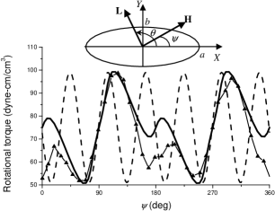
Figure 1: Rotational torque of untwinned NiO crystal at RT in H=4.8 kOe for [111] rotational axis. Triangles - experimental data Roth:1960(2) , solid line – theoretical approximation according to (8), (9), dashed line – approximation of infinite crystal (no shape effect).

Analysis of eqs. (8)-(9) shows that i) effective anisotropy is determined by shape-dependent (via $a/b$ ratio) constants $K^{\rm elas}_{\rm 2}$, $K^{\rm elas}_{\rm 4an}$; ii) shape-induced anisotropy removes multiaxial degeneracy of equilibrium orientation of antiferromagnetic vector and thus excludes formation of domain structure; iii) in the field absence the preferred orientation of antiferromagnetic vector coincides with the longer ellipse axis ($K^{\rm elas}_{\rm 2}>0$, $a>b$); iv) external magnetic field applied along the longer ellipse axis may induce spin-flop transition at $H=H_{\rm{SF}}$, where spin-flop field

$$H_{\rm{SF}}=\sqrt{\frac{1}{\chi}\left|{K_{2}^{\rm{elas}}-4K_{4\rm{an}}^{\rm{elas}}}\right|}\propto{\frac{\lambda^{\prime}}{\sqrt{\chi c_{44}}}}\sqrt{\frac{a-b}{a+b}}$$ (10)

is governed by the sample shape and is independent of crystalline anisotropy.

An interesting result is obtained for the sample having a square cross-section. In this case equilibrium distribution of antiferromagnetic vector is in principle inhomogeneous but in average can still be described by eq. (9) with

$$K^{\rm elas}_{2}=0,\qquad K^{\rm elas}_{\rm 4an}=\frac{\ln 2(\lambda^{\prime})^{2}}{\pi c_{44}(1-\nu)}>0\,.$$ (11)

It is obvious that such a sample shows 4-th order effective anisotropy with “easy axes” directed along square diagonal (45^∘ angle with respect to $X$ axis, as results from condition $K^{\rm elas}_{\rm 4an}>0$).

The rotational torque calculated from eqs. (8), (9) for a typical antiferromagnet NiO is shown in figs. 1, 2. In calculations we use experimental results Roth:1960(2) for a rotational torque around [111] axis taken at room temperature for $H$=4.8 kOe (triangles in fig. 1). Since the experiment shows strong hysteresis in clock-wise and counter-clock wise rotations, the data in fig. 1 are preliminarily averaged over cc-ccw cycle. Theoretical curve (solid line) includes some nonzero average torque that may result from inhomogeneity of the sample, and adjusting parameters are $\chi=4.35\cdot 10^{-4}$ emu/cm³, $K_{2}^{\rm{elas}}=900$ erg/cm³, $K_{4\rm{an}}^{\rm{elas}}=450$ erg/cm³, $a/b=20$.

Four curves in fig. 2 demonstrate possible variation of the rotational torque with the crystal shape. For a large aspect ratio (curve (a)) contributions from both 2-nd and 4-th order anisotropy terms are equally important ($K_{2}^{\rm{elas}}\propto K_{4\rm{an}}^{\rm{elas}}$), the torque curve is composed of $\sin 2\theta$ and $\sin 4\theta$ components. At lower aspect ratio (curves (b), (c)) the 4-th order component becomes less pronounced and the amplitude of torque also diminishes. A circular cylinder ($a=b$) will show no shape effect in a single domain state, but a sample with a square cross-section should posses 4-th order anisotropy (as seen from curve (d)) regardless of crystalline symmetry.

Figure 2: Rotational torque (calculated) of untwinned NiO crystal at RT in H=5 kOe for [111] rotational axis for the samples with different shape. For ellipse-section samples an aspect ratio is $a/b=20$ (a); 3 (b); 1.2 (c); (d) – square-section sample.

Evidently, shape-dependence of the magnetic rotational torque for NiO crystal was observed in Ref. Roth:1960(2), . The authors notice that “a nearly pure $\sin 4\theta$ curve is obtained when the (111) cross section is square”. For an arbitrary shaped section the experimental curve (fig. 1, triangles) is satisfactorily fitted with combination of $\sin 2\theta$ and $\sin 4\theta$ components (solid line). Dashed line in fig. 1 shows theoretical curve with $f_{\rm{in-plane}}^{\rm{mag}}=220\cos 6\theta$ erg/cm³ that could be expected in neglecting of shape-induced effects. The presence of $\sin 4\theta$ component in the rotational torque makes it possible to exclude the effect of $\mathbf{L}$ “freezing” by magnetoelastic strain which may be expected in relatively small magnetic field. Additional anisotropy induced by frozen lattice is uniaxial and should be insensible to the variation of a crystal shape.

VI Antiferromagnetic resonance

The effect of shape-induced anisotropy may also be detected by measuring frequency of the lowest branch of a spin-wave spectrum. Antiferromagnetic resonance (AFMR) frequency calculated within a standard Lagrangian technique in long-wave approximation is given by the expression

$$\nu_{\rm AFMR}=g\sqrt{\frac{2}{\chi}\left(K_{\rm{is}}^{\rm{elas}}+{K_{2}^{\rm{elas}}\cos 2\theta+4K_{4\rm{an}}^{\rm{elas}}\cos 4\theta-\chi H^{2}\cos 2(\theta-\psi)}\right)},$$ (12)

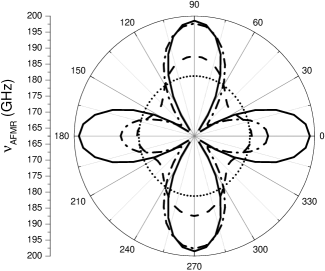
Figure 4: Angular dependence of AFMR frequency vs magnetic field orientation for samples with different aspect ratio: $a/b=20$ (dash-dotted line); 3 (dashed line); 1.2 (dotted line). Solid line corresponds to a square-section sample.

where $g$ is gyromagnetic ratio and equilibrium value of $\theta$ may be calculated from (9). Polar diagram of $\nu_{\rm AFMR}(\psi)$ calculated from (12) for NiO ($g=2,5$) for a different crystal shape is shown in fig. 4. For the aspect ratio close to 1 (dotted line) the shape effect is negligible and magnetoelastic gap in AFMR spectrum is almost isotropic. For elongated (dash-dotted and dashed lines) or square-shaped (solid line) samples the AFMR gap should show strong 2-fold or 4-fold anisotropy.

VII Shape effect in antiferromagnetic nanopillars

Taking into account recent interest to multilayered structures based on antiferromagnetic materials we consider possible shape effects in antiferromagnetic nanopillar that can be a constitutive part of spin-valve structure (see, e.g. Urazhdin:2007 ). Typical nanopillar has a form of a very thin (thickness $c\approx 3\div 10$ nm) elliptic cylinder with the pronounced in-plane aspect ratio (with $a\propto 120$ nm and $b\propto 50$ nm).

In this case ($c\ll a,b$) the constants of shape-induced anisotropy may be expressed through the parameter $k^{2}=1-b^{2}/a^{2}$ that depends on the aspect ratio $b/a\leq 1$, namely,

$$K^{\rm elas}_{2}=\frac{c}{b}\cdot\frac{[(\lambda^{\prime})^{2}(2-3\nu)+\lambda_{v}\lambda^{\prime}]J_{2}(k)}{4c_{44}(1-\nu)},\,K^{\rm elas}_{\rm 4an}=\frac{c}{b}\cdot\frac{2(\lambda^{\prime})^{2}J_{4}(k)}{3c_{44}(1-\nu)}\,,$$ (13)

where we have introduced the dimensionless shape-factors $J_{2,4}$ as follows

$$J_{2}(k) = \int_{0}^{\pi/2}\frac{(\sin^{2}\phi+\cos 2\phi/k^{2})d\phi}{\sqrt{1-k^{2}\sin^{2}\phi}},$$

$$J_{4}(k) = \int_{0}^{\pi/2}\frac{(1-8\cos 2\phi-k^{2}\sin^{2}\phi+8\cos 2\phi/k^{2})d\phi}{\sqrt{1-k^{2}\sin^{2}\phi}}.$$ (14)

Figure 3: The 2-nd (a) and 4-th order (b) shape-induced anisotropy of thin nanopillar as a function of aspect ratio. Arrow indicates the typical value of $b/a$ used in the experiments Urazhdin:2007 .

Dependence of the shape-factors $J_{2,4}$ vs aspect ratio calculated according to eq. (VII) is given in Fig.3. It can be easily understood that both shape-induced constants (13) vanish for isotropic sample ($b=a$). For all the values of aspect ratio the 2-nd order term is greater than that of the 4-th order, $J_{2}\geq J_{4}$. In the experimentally accessible range of values $b\propto 0.5a$ $J_{2}=0.52$ and $J_{4}=0.3$. Thus, characteristic value of the shape-induced anisotropy in the stress-free thin film can be of the order magnetoelastic energy $K_{\rm{is}}^{\rm{elas}}\propto(\lambda^{\prime})^{2}/c_{44}$ multiplied by small factor $c/b$ that varies within the range 0.05$\div$0.3 depending on the film thickness.

Substantial enhancement of the 2nd order shape-induced anisotropy $K^{\rm elas}_{2}$ should be expected in the case of mismatch between antiferromagnet and substrate lattices. Lattice misfit is a source of rather strong (usually isotropic) in-plane stresses $\sigma^{\rm mf}_{xx}=\sigma^{\rm mf}_{yy}=\sigma^{\rm mf}$ that should be added to the intrinsic stresses (3). Corresponding (and principal) contribution into the effective 2-nd order anisotropy constant takes a form

$$K^{\rm elas}_{2}=\frac{c}{b}\cdot\frac{\sigma^{\rm mf}\lambda^{\prime}J_{2}(k)}{4c_{44}(1-\nu)}.$$ (15)

If $u^{\rm mf}$ is lattice mismatch and $u^{\rm spon}\propto\lambda^{\prime}/c_{44}$ is an observable spontaneous strain that occurs in the Néel point, then, we can estimate $\sigma^{\rm mf}\propto c_{44}u^{\rm mf}$ (in assumption that the elastic modula of substrate and antiferromagnet are of the same order of value), $K_{\rm{is}}^{\rm{elas}}\propto(\lambda^{\prime})^{2}/c_{44}$ and hence,

$$K^{\rm elas}_{2}\propto\frac{c}{b}\frac{u^{\rm mf}}{u^{\rm spon}}K_{\rm{is}}^{\rm{elas}}.$$

Substituting typical values of small lattice misfit $u^{\rm mf}=0.005$ and large spontaneous striction $u^{\rm spon}=10^{-4}$ we see that even for very thin nanopillars with $c/b=0.05$ shape induced anisotropy may be as large as $K^{\rm elas}_{2}=2.5K_{\rm{is}}^{\rm{elas}}$ and thus much greater than the “bare” in-plane magnetic anisotropy of antiferromagnet (see table 1).

Nontrivial relation (15) between the shape of the sample and external stress produced by the substrate may reveal itself in switching of the shape-induced direction of easy axis for different substrates. Really, if $K^{\rm elas}_{2}>0$, then, equilibrium orientation of $\mathbf{L}$ in monodomain sample is parallel to the ellipse’s long axis $a$ ($X$-direction), as can be seen from (4) and inset in fig. 1. According to equation (15), the sign of $K^{\rm elas}_{2}$ depends upon the relation between intrinsic ($\lambda^{\prime},u^{\rm spon}$) and extrinsic ($\sigma^{\rm mf},u^{\rm mf}$) stresses (or strains). In the case when both substrate and eigen magnetoelastic forces of antiferromagnet “work” in the same direction, trying to extend (compress) crystal lattice, product $\sigma^{\rm mf}\lambda^{\prime}$ will be positive (in accordance with Le Chatelier principle) and $K^{\rm elas}_{2}>0$. If we use another substrate which produces misfit of opposite sign, $K^{\rm elas}_{2}<0$ and equilibrium orientation of $\mathbf{L}$ will be parallel to the short axis $b$ ($Y$-direction).

Controlling of spin-orientation by substrate-induced strain was recently observedCsisza:2005 in antiferromagnet CoO. In bulk samples CoO is compressed in $\mathbf{L}$ direction. When grown on Mg(100) substrate, CoO lattice is expanded in plane and experiment shows that Co spin go out of plane. And on contrary, in-plane ordering is observed for Ag(100) substrate, which produces slight contraction in the film plane. From our point of view, analogous experiments with nanopillars can be very instructive in further study of shape-induced effect in antiferromagnetic crystals.

VIII Conclusions

In summary, we propose a model that describes an antiferromagnet with the pronounced magnetoelastic coupling. The model is based on the assumption that antiferromagnetic ordering is accompanied by appearance of elastic dipoles. Due to the long-range nature of elastic forces, the energy of dipole-dipole interaction (destressing energy) in the finite-size sample depends on the crystal shape and is proportional to its volume.

In the “easy-plane” antiferromagnets with degenerated orientation of easy axis the destressing effects may stimulate formation of the domain structure and re-distribution of the domains in the presence of external magnetic field.

The model predicts existence of the shape-induced magnetic anisotropy which corresponds to macroscopic symmetry of the sample and can be detected by the magnetic rotational torque and AFMR measurements.

Crystal shape may be a source of additional magnetic uniaxial anisotropy which produces different effects depending of aspect ratio. Below some critical value of $a/b$ shape-induced anisotropy favors formation of the domain structure even in the absence of any external field. For large aspect ratio (above the critical value) shape-induced anisotropy removes degeneracy of easy-axis in a single domain sample. Energy difference between thus induced easy- and hard-directions depends upon $a/b$. Square cross section sample should acquire 4th order anisotropy (irrespective to the crystal symmetry in easy plane). This opens a possibility to control macroscopic properties of the sample varying its shape.

The shape of antiferromagnetic nanopillars imbedded into structures with lattice mismatch may be a principal source of magnetic anisotropy. This fact should be taken into account in engineering of spin-valve devices.

References

- (1) Néel L., Proc. International Conf. Theor. Physics. Kyoto and Tokyo. Science Council of Japan, Tokyo. 701 (1953).
- (2) Wilkinson M. K., Cable J. W., Wollan E. O. and Koehler W. C., Phys. Rev 113, 497 (1959).
- (3) Tanner B. K., Safa M., Midgley D. and Bordas J., JMMM 1, 337 (1976).
- (4) Baruchel J., Schlenker M. and Roth W. L., J. Appl. Phys 48, 5 (1977).
- (5) Janossy A., Simon F., Feher T., Rockenbauer A., Korecz L., Chen C., Chowdhury A. J. S. and Hodby J.W., Phys. Rev. B 59, 1176 (1999).
- (6) Scholl A., Stöhr J., Lüning J., Seo J. W., Fompeyrine J., Siegwart H., Locquet J. P., Nolting F., Anders S., Fullerton E. E, Schneifein M. R. and Padmore H. A., Science 287, 1014 (2000).
- (7) Weber N. B., Bethke C. and Hillebrecht F. U., JMMM 226, 1573 (2001).
- (8) Li Y. Y., Phys. Rev 101, 1450 (1956).
- (9) Kalita V. M., Losenko A. F., Ryabchenko S. M., Trotsenko P. A. and Yatkevich T. M., Fizika tverdogo tela 46, 317 (2004).
- (10) Gomonay H. V. and Loktev V. M., Physics of the Solid State 47, 1755 (2005).
- (11) Kléman M. and Schlenker M., J. Appl. Phys. 43, 3184 (1972).
- (12) Gomonay H. V. and Loktev V. M., J. Physics: Cond. Matter 14, 3959 (2002).
- (13) Roth W. L. and Slack G. A., J. Appl. Phys 31, S352 (1960).
- (14) Urazhdin S. and Anthony N., cond-mat/0703281v1.
- (15) Csiszar S. I., Haverkort M. W., Hu Z., Tanaka A., Hsieh H. H., Lin H.-J., Chen C. T., Hibma T., and Tjeng L. H., Phys. Rev. Lett. 95, 187205 (2005).