The anisotropic XY model on the inhomogeneous periodic chain

Abstract

The static and dynamic properties of the anisotropic XY-model $(s=1/2)$ on the inhomogeneous periodic chain, composed of $N$ cells with $n$ different exchange interactions and magnetic moments, in a transverse field $h,$ are determined exactly at arbitrary temperatures. The properties are obtained by introducing the Jordan-Wigner fermionization and by reducing the problem to a diagonalization of a finite matrix of $nth$ order. The quantum transitions are determined exactly by analyzing, as a function of the field, the induced magnetization $1/n\sum_{m=1}^{n}\mu_{m}\left\langle S_{j,m}^{z}\right\rangle$ ( $j$ denotes the cell, $m$ the site within the cell, $\mu_{m}$ the magnetic moment at site $m$ within the cell) and the spontaneous magnetization $1/n\sum_{m=1}^{n}\left\langle S_{j,m}^{x},\right\rangle$ which is obtained from the correlations $\left\langle S_{j,m}^{x}S_{j+r,m}^{x}\right\rangle$ for large spin separations. These results, which are obtained for infinite chains, correspond to an extension of the ones obtained by Tong and Zhong(Physica B 304, 91 (2001)). The dynamic correlations, $\left\langle S_{j,m}^{z}(t)S_{j^{\prime},m^{\prime}}^{z}(0)\right\rangle$, and the dynamic susceptibility, $\chi_{q}^{zz}(\omega),$ are also obtained at arbitrary temperatures. Explicit results are presented in the limit $T=0$, where the critical behaviour occurs, for the static susceptibility $\chi_{q}^{zz}(0)$ as a function of the transverse field $h$, and for the frequency dependency of dynamic susceptibility $\chi_{q}^{zz}(\omega)$.

identifier

I Introduction

The one-dimensional XY-model introduced by Lieb, Schultz and Mattis lieb:1961 is still one of the few quantum many-body problems  that can be solved exactly. Although almost forty-five years have passed since the original solution has been proposed, this old model continues to provide new information on the quantum behaviour of magnetic systemsdagotto:1996 ; nguyen:1996 ; gambardella:2002 ; mukherjeea:2004 ; matsumoto:2004 . In particular, it has shed some light on the quantum phase transitions sachdev:2000 , since exact results can be obtained for most of its properties. The model has also been applied in the study of quantum entanglement, which plays an essential role in the quantum computation. Important results of this application can be found in the recent work by Amico et al.Amico:2006  and in the references therein.

In this paper we will consider the anisotropic XY-model in a transverse field on the inhomogeneous periodic (closed) chain consisting of $N$ cells composed  of $n$ sites, whose version on the open chain has been recently addressed by Feldmanfeldman:2006 . It has also been studied by Tong and Zhong tongzhong:2001 and Derzhko et al.derzhko:2004 , who have restricted their analysis to the study of the thermodynamic properties. To the best of our knowledege, the work  by Tong and Liutongliu:2006 , which concerns the study of the zeros of the partition function, at T=0, and its relation to the quantum phase transitions contains the latest results on the model.

The anisotropic model corresponds to an extension of the isotropic one recently studied by the authorsdelima:2006 . Its study on the inhomogeneous periodic chain also corresponds to an extension of its version on the alternating superlatticesiskens:1975 ; perk:1975 ; perk:1980 ; taylor:1985 ; barbosafilho:2001 ; delima:2002 , and, in this work, we will solve exactly the model by considering $n$ different exchange constants and magnetic moments. The aim of this work is to present a comprehensive study of its static and dynamic quantum critical behaviour.

In Section 2 we introduce the model and diagonalize its Hamiltonian. An explicit expression is presented for $n=2,$ and the results compared to the known ones obtained by various authors siskens:1975 ; perk:1975 ; perk:1980 ; taylor:1985 ; barbosafilho:2001 ; delima:2002 . We also present the solution of the model for $n=8$, which has been obtained numerically.

The induced magnetization $M^{z}$ and  the isothermal susceptibility $\chi_{T}^{zz},$ at arbitrary temperature, are obtained in Section 3, and explicit expressions presented for $T=0$. By analyzing these quantities, the quantum critical behaviour is studied and the critical exponents associated to the quantum transitions are obtained.

The spontaneous magnetization $M^{x}$ is obtained in Section 4, from the two-spin correlation $\left\langle S_{l,m}^{x}S_{l+r,m}^{x}\right\rangle,$ and the critical behaviour is also obtained, with high accuracy, numerically, by means of a non-linear regression of the data evaluated for finite values of $r$. This rather surprising result allows for the complete determination of $M^{x}$ as a function of the field, and to determine the multiple quantum transitions undergone by the model.

The static and dynamic correlations $\left\langle\tau_{l}^{z}\tau_{l+r}^{z}\right\rangle$ are presented in Section 5 and, the dynamic susceptibility $\chi_{q}^{zz}(\omega),$ in Section 6. Finally, in Section 7, we summarize the main results of the paper.

II The model

We consider the anisotropic XY- model $(s=1/2)$ on the inhomogeneous periodic chain with $N$ cells, $n$ sites per cell, and lattice parameter $a$, in a transverse field, whose unit cell is shown in Fig. 1, which corresponds to an extension of the isotropic model recentely considered delima:2006 . The Hamiltonian is given by

$$H =-\sum_{l=1}^{N}\left\{\sum_{m=1}^{n}\mu_{m}hS_{l,m}^{z}+\left[\sum_{m=1}^{n-1}J_{m}\left(1+\gamma_{m}\right)S_{l,m}^{x}S_{l,m+1}^{x}+J_{m}\left(1-\gamma_{m}\right)S_{l,m}^{y}S_{l,m+1}^{y}\right]\right.+$$

$$\left.+J_{n}\left(1+\gamma_{n}\right)S_{l,n}^{x}S_{l+1,1}^{x}+J_{n}\left(1-\gamma_{n}\right)S_{l,n}^{y}S_{l+1,1}^{y}\right\},$$ (1)

Figure 1: Unit cell of the inhomogeneous periodic chain

where the parameters $J_{l,m}$ are the exchange couplings between nearest-neighbour, $\mu_{m}$ the magnetic moments, $h$ the external field, and we have assumed periodic boundary conditions. If we introduce the ladder operators

$$S_{l,m}^{\pm}=S_{l,m}^{x}\pm iS_{l,m}^{y},$$ (2)

and the generalized Jordan-Wigner transformationgoncalves:1995

$$S_{l,m}^{{}^{+}} =\exp\left\{i\pi\sum_{l^{\prime}=1}^{l-1}\sum_{m^{\prime}=1}^{n}c_{l^{\prime},m^{\prime}}^{\dagger}c_{l^{\prime},m^{\prime}}+i\pi\sum_{m^{\prime}=1}^{m-1}c_{l,m^{\prime}}^{\dagger}c_{l,m^{\prime}}\right\}c_{l,m}^{\dagger},$$

$$S_{l,m}^{z} =c_{l,m}^{\dagger}c_{l,m}-\frac{1}{2},$$ (3)

where $c_{l,m}$ and $c_{l,m}^{\dagger}$ are fermion annihilation and creation operators, we can write the Hamiltonian assiskens:1974

$$H=H^{+}P^{+}+H^{-}P^{-},$$ (4)

where

$$H^{\pm} =-\sum_{l=1}^{N}\left\{\sum_{m=1}^{n}\mu_{m}h\left(c_{l,m}^{\dagger}c_{l,m}-\frac{1}{2}\right)\right.+\sum_{m=1}^{n-1}\left[\frac{J_{m}}{2}\left(c_{l,m}^{\dagger}c_{l,m+1}+c_{l,m+1}^{{\dagger}}c_{l,m}\right)\right.+$$

$$\left.\left.+\frac{J_{m}\gamma_{m}}{2}\left(c_{l,m}^{\dagger}c_{l,m+1}^{\dagger}+c_{l,m+1}c_{l,m}\right)\right]\right\}-\sum_{l=1}^{N-1}\left[\frac{J_{n}}{2}\left(c_{l,n}^{\dagger}c_{l+1,1}+c_{l+1,1}^{\dagger}c_{l,n}\right)\right.+$$

$$\left.+\frac{J_{n}\gamma_{n}}{2}\left(c_{l,n}^{\dagger}c_{l+1,1}^{\dagger}+c_{l+1,1}c_{l,n}\right)\right]\pm\left[\frac{J_{n}}{2}\left(c_{N,n}^{\dagger}c_{1,1}+c_{1,1}^{\dagger}c_{N,n}\right)+\frac{J_{n}\gamma_{n}}{2}\left(c_{N,n}^{\dagger}c_{1,1}^{\dagger}+c_{1,1}c_{N,n}\right)\right],$$ (5)

and

$$P^{\pm}=\frac{I\pm P}{2},$$ (6)

with $P$ given by

$$P=\exp\left(i\pi\sum_{l=1}^{N}\sum_{m=1}^{n}c_{l,m}^{\dagger}c_{l,m}\right).$$ (7)

As it is well known siskens:1974 ; capel:1977 ; goncalvestese:1977 , since the operator $P$ commutes with the Hamiltonian, the eigenstates have definite parity, and $P^{-}(P^{+})$ corresponds to a projector into a state of odd (even) parity.

Introducing periodic and anti-periodic boundary conditions on $c^{\prime}s$ for $H^{-}$ and $H^{+}$ respectively, the wave-vectors in the Fourier transform barbosafilho:2001 ,

$$c_{l,m} =\frac{1}{\sqrt{N}}\sum_{q}\exp\left(-iqdl\right)a_{q,m},$$

$$a_{q,m} =\frac{1}{\sqrt{N}}\sum_{l=1}^{N}\exp\left(iqdl\right)c_{l,m},$$ (8)

are given by $q^{-}=\frac{2l\pi}{Nd},$ for periodic condition and $q^{+}=\frac{\pi(2l+1)}{Nd}$, for anti-periodic condition, with $l=0,\pm 1,....,\pm N/2$, and $H^{-}$ and $H^{+}$ can be written in the form

$$H^{\pm}=\sum_{q^{\pm}}H_{q^{\pm}},$$ (9)

where

$$H_{q^{\pm}} =-\sum_{m=1}^{n}\mu_{m}h\left(a_{q^{\pm},m}^{\dagger}a_{q^{\pm},m}-\frac{1}{2}\right)-$$

$$-\sum_{m=1}^{n-1}\frac{J_{m}}{2}\left[a_{q^{\pm},m}^{\dagger}a_{q^{\pm},m+1}+a_{q^{\pm},m+1}^{\dagger}a_{q^{\pm},m}+\gamma_{m}\left(a_{q^{\pm},m}^{\dagger}a_{q^{\pm},m+1}^{\dagger}+a_{q^{\pm},m+1}a_{q^{\pm},m}\right)\right]-$$

$$-\frac{J_{n}}{2}\left[a_{q^{\pm},n}^{\dagger}a_{q^{\pm},1}\exp(-idq^{\pm})+a_{q^{\pm},1}^{\dagger}a_{q^{\pm},n}\exp(idq^{\pm})\right.+$$

$$+\left.\gamma_{m}\left(a_{q^{\pm},n}^{\dagger}a_{q^{\pm},1}^{\dagger}\exp(-idq^{\pm})+a_{q^{\pm},1}a_{q^{\pm},n}\exp(idq^{\pm})\right)\right].$$ (10)

Although $H^{-}$ and $H^{+}$ do not commute, it can be shown that in the thermodynamic limit all the static properties of the  system can be obtained in terms of $H^{-}$ or $H^{+}.$ However, even in this limit, some dynamic properties depend on $H^{-}$ and $H^{+}$ siskens:1974 ; capel:1977 ; goncalvestese:1977 . Since $\left[H_{q^{\pm}},H_{-q^{\pm}}\right]\neq 0,$ we consider the symmetrization

$$\widetilde{H}_{q^{\pm}}\equiv H_{q^{\pm}}+H_{-q^{\pm}},$$ (11)

and the Hamiltonian $H^{\pm}$ can be written as

$$H^{\pm}=\frac{1}{2}{\displaystyle\sum\limits_{q^{\pm}}}\widetilde{H}_{q^{\pm}}.$$ (12)

By making the identification $q^{\pm}\equiv q,$ it follows immediately that $\left[\widetilde{H}_{q},\widetilde{H}_{q^{\prime}}\right]=0.$ Therefore, following the procedure introduced by Lieb, Schultz and Mattis lieb:1961 , we can diagonalize the Hamiltonian $H^{\pm}$ by introducing the canonical transformation

$$a_{q,m} =\sum\limits_{k}^{n}\left(\frac{\psi_{q,k,m}^{\ast}+\phi_{q,k,m}^{\ast}}{2}\eta_{q,k}+\frac{\psi_{q,k,m}^{\ast}-\phi_{q,k,m}^{\ast}}{2}\eta_{-q,k}^{\dagger}\right),$$

$$a_{q,m}^{\dagger} =\sum\limits_{k}^{n}\left(\frac{\psi_{q,k,m}+\phi_{q,k,m}}{2}\eta_{q,k}^{\dagger}+\frac{\psi_{q,k,m}-\phi_{q,k,m}}{2}\eta_{-q,k}\right),$$ (13)

where $\mathbf{\phi}_{q,k,m}$ and $\mathbf{\psi}_{q,k,m}$ are the components of the eigenvectors, $\mathbf{\Phi}_{q,k}$ and $\mathbf{\Psi}_{q,k}$, of the matrices $\left(\mathbb{A}_{q}-\mathbb{B}_{q}\right)\left(\mathbb{A}_{q}+\mathbb{B}_{q}\right)$ and $\left(\mathbb{A}_{q}+\mathbb{B}_{q}\right)\left(\mathbb{A}_{q}-\mathbb{B}_{q}\right),$ with $\mathbb{A}_{q}$ and $\mathbb{B}_{q}$ given by

$$\mathbb{A}_{q}=-\left(\begin{array}[c]{llllll}\mu_{1}h&\frac{J_{1}}{2}&0&\cdots&0&\frac{J_{n}}{2}\exp\left(iqd\right)\\ \frac{J_{1}}{2}&\mu_{2}h&\frac{J_{2}}{2}&&&0\\ 0&\frac{J_{2}}{2}&\mu_{3}h&\frac{J_{3}}{2}&&\vdots\\ \vdots&&\frac{J_{3}}{2}&\ddots&\ddots&0\\ 0&&&\ddots&\mu_{n-1}h&\frac{J_{n-1}}{2}\\ \frac{J_{n}}{2}\exp\left(-iqd\right)&0&\cdots&0&\frac{J_{n-1}}{2}&\mu_{n}h\end{array}\right),$$ (14)

$$\mathbb{B}_{q}=\left(\begin{array}[c]{llllll}0&-\frac{J_{1}\gamma_{1}}{2}&0&\cdots&0&\frac{J_{n}\gamma_{n}}{2}\exp\left(iqd\right)\\ \frac{J_{1}\gamma_{1}}{2}&0&-\frac{J_{2}\gamma_{2}}{2}&&&0\\ 0&\frac{J_{2}\gamma_{2}}{2}&0&-\frac{J_{3}\gamma_{3}}{2}&&\vdots\\ \vdots&&\frac{J_{3}\gamma_{3}}{2}&\ddots&\ddots&0\\ 0&&&\ddots&0&-\frac{J_{n-1}\gamma_{n-1}}{2}\\ -\frac{J_{n}\gamma_{n}}{2}\exp\left(-iqd\right)&0&\cdots&0&\frac{J_{n-1}\gamma_{n-1}}{2}&0\end{array}\right).$$ (15)

The corresponding eigenvalues are $E_{q,k}^{2},$ the squares of the fermion energy levels, such that the Hamiltonian $H^{\pm},$ given in eq.(10), can be written in the diagonal form

$$H^{\pm}=\sum_{q,k}E_{q,k}\left(\eta_{q,k}^{\dagger}\eta_{q,k}-\frac{1}{2}\right),$$ (16)

where for $H^{+}(H^{-})$ the wave-vector $q$ is identical to $q^{+}(q^{-}),$ and the spectrum $E_{q,k}$ of $\ \widetilde{H}_{q}$ is determined from the determinantal equation

$$\det\left[\left(\mathbb{A}_{q}+\mathbb{B}_{q}\right)\left(\mathbb{A}_{q}-\mathbb{B}_{q}\right)-E_{q}^{2}\mathbb{I}\right]=0.$$ (17)

Since we are interested in the thermodynamic limit, we will consider from here on $H^{-}$ only, in all calculations.

Explicit expressions for the excitation spectrum can be determined for $n$ equal to 2, 3 and 4, and for $n$ greater than 4, it is determined numerically from eq.(17). Since we are considering the particle-hole representation, this implies that $E_{q}\geqslant 0.$

Explicitly, for $n=2$, the excitation spectrum is given by

$$E_{q}^{2} =\frac{\alpha_{1}+\alpha_{2}+(\lambda_{1}+\lambda_{2})\cos 2q}{2}\pm$$

$$\frac{1}{2}\sqrt{\left[\alpha_{1}-\alpha_{2}+(\lambda_{1}-\lambda_{2})\cos 2q\right]^{2}+4\left[\delta_{1}^{2}+\delta_{2}^{2}+2\delta_{1}\delta_{2}\cos(2q)\right]},$$ (18)

where

$$\alpha_{1} =(\mu_{1}h)^{2}+\frac{J_{1}^{2}}{4}(1+\gamma_{1})^{2}+\frac{J_{2}^{2}}{4}(1-\gamma_{2})^{2},$$

$$\alpha_{2} =(\mu_{2}h)^{2}+\frac{J_{2}^{2}}{4}(1+\gamma_{2})^{2}+\frac{J_{1}^{2}}{4}(1-\gamma_{1})^{2},$$

$$\lambda_{1} =\frac{J_{1}J_{2}}{2}(1+\gamma_{1})(1-\gamma_{2}),$$

$$\lambda_{2} =\frac{J_{1}J_{2}}{2}(1-\gamma_{1})(1+\gamma_{2}),$$

$$\delta_{1} =\frac{J_{1}}{2}(1-\gamma_{1})\mu_{1}h+\frac{J_{1}}{2}(1+\gamma_{1})\mu_{2}h,$$

$$\delta_{2} =\frac{J_{2}}{2}(1+\gamma_{2})\mu_{1}h+\frac{J_{2}}{2}(1-\gamma_{2})\mu_{2}h.$$ (19)

For $\gamma_{1}=\gamma_{2}=0,$ the previous result reproduces the excitation spectrum obtained for the isotropic case delima:2006 , provided we consider the particle representation which allows for negative energies. It also reproduces the result obtained by Siskens et al.siskens:1975 .

As already pointed out, although explicit expressions can be determined for $n$ equal to 3 and 4, they are not presented here since they are too cumbersome.

Even in the case where we have identical magnetic moments, differently from the isotropic case, the effect of the the field does not correspond to a translation of the excitation spectrum for zero field, since the term of the field does not commute with the Hamiltonian.

The critical fields which characterize the quantum transitions are determined from the excitation spectrum by imposing the condition $E_{q}=0$ for $q=0$ and $q=\pi/d$delima:2006 . The number of transitions is highly dependent on the anisotropy and varies from $n$ to one. In particular, the limit of a single transition always occurs for the transverse Ising model which corresponds to the $\gamma^{\prime}s$ equal to one.

The excitation spectrum for $n=8$ and identical magnetic moments is presented in Fig.2 for identical and different $\gamma^{\prime}s$, where we have considered the lattice spacing $a=1.$ As it can be seen, the energy of the modes is always positive and the effect of the spatial variation of the anisotropy is more pronounced in the low energy modes. Since there is no zero energy excitation, the model is not critical at the considered value of the transverse field.

Figure 2: Excitation spectrum for $n=8,J_{1}=J_{6}=J_{8}=1.5,$ $J_{2}=3,$ $J_{3}=1.5,$ $J_{4}=$ $J_{5}=J_{7}=2,$ $h=1$, $\mu_{1}=...=\mu_{8}=1$ and $\gamma_{1}=...=\gamma_{8}=0.1$ (continuous line), and for $\gamma_{1}=0.1,$ $\gamma_{2}=0.2,$ $\gamma_{3}=0.3,$ $\gamma_{4}=0.4,\gamma_{5}=0.5,$ $\gamma_{6}=0.6,\gamma_{7}=0.7,$ $\gamma_{8}=0.8$ (dashed line).

III The induced magnetization and isothermal susceptibility $\chi_{T}^{zz}$

From eqs.(3), the operator $S_{l,m}^{z}$ can be written as

$$S_{l,m}^{z}=-\frac{1}{2}A_{l,m}B_{l,m},$$ (20)

with

$$A_{l,m} \equiv c_{l,m}^{\dagger}+c_{l,m},$$

$$B_{l,m} \equiv c_{l,m}^{\dagger}-c_{l,m},$$ (21)

which can be expressed, from eqs.(8)and (13), as

$$A_{l,m} =\frac{1}{\sqrt{N}}\sum_{q,k}e^{iqdl}\psi_{q,k,m}\left(\eta_{q,k}^{\dagger}+\eta_{-q,k}\right),$$

$$B_{l,m} =\frac{1}{\sqrt{N}}\sum_{q,k}e^{iqdl}\phi_{q,k,m}\left(\eta_{q,k}^{\dagger}-\eta_{-q,k}\right).$$ (22)

By using eqs.(20) and (22), the local magnetization $M_{l,m}^{z}$ can be written as

$$M_{l,m}^{z}\equiv\mu_{m}\left\langle S_{l,m}^{z}\right\rangle=-\frac{1}{2N}\sum\limits_{q,k}\mu_{m}\psi_{q,k,m}\phi_{q,k,m}^{\ast}\left(1-2n_{q,k}\right),$$ (23)

where the fermion occupation number $n_{q,k}$ is given by

$$n_{q,k}=\frac{1}{1+e^{\overline{E}_{q,k}}},$$ (24)

where $\overline{E}_{q,k}=\beta E_{q,k}\equiv E_{q,k}/k_{B}T$, and the calculation has been done by considering $H=H^{-}$ siskens:1974 ; capel:1977 ; goncalvestese:1977 , since we are interested in the thermodynamic limit.

As in the isotropic model delima:2006 , we define an average cell magnetization operator in the $z$ direction, $\tau_{l}^{z},$ as

$$\tau_{l}^{z}\equiv\frac{1}{n}\sum_{m=1}^{n}\mu_{m}S_{l,m}^{z},$$ (25)

then the induced magnetization per site, $M^{z},$ is equal to $\left\langle\tau_{l}^{z}\right\rangle$ and, from eq.(23), can be written in the form

$$M^{z}\equiv\left\langle\tau_{l}^{z}\right\rangle=-\frac{1}{2nN}\sum\limits_{q,k,m}\mu_{m}\psi_{q,k,m}\phi_{q,k,m}^{\ast}\tanh\left(\frac{{}^{\overline{E}_{q,k}}}{2}\right),$$ (26)

which at $T=0$ becomes

$$M^{z}=-\frac{1}{2nN}\sum\limits_{q,k,m}\mu_{m}\psi_{q,k,m}\phi_{q,k,m}^{\ast}.$$ (27)

The isothermal susceptibility can be obtained from eqs.(26) and (27) by means of the expression

$$\chi_{T}^{zz}\equiv\frac{1}{n}\frac{\partial M^{z}}{\partial h},$$ (28)

which has to be evaluated numerically.

Figure 3: (a) Magnetization $M^{z}$ and (b) isothermal susceptibility $\chi_{T}^{zz},$at $T=0,$ as functions of the field for $n=8,$ $\mu_{1}=...=\mu_{8}=1$, $J_{1}=J_{6}=J_{8}=1.5,$ $J_{2}=3,$ $J_{3}=1.5,$ $J_{4}=$ $J_{5}=J_{7}=2,$ $\gamma=0.1$(dashed line) and for $\gamma=0.15$(continuous line).

At $T=0,$ the isothermal susceptibility $\chi_{T}^{zz}$ diverges at the quantum critical points induced by the field. This result can be seen in Fig.3 where $M^{z}$ and $\chi_{T}^{zz}$ are presented as functions of the field $h,$ at $T=0$, for a chain with $n=8$, identical $\mu$’s, $\gamma=0.1$ and $0.15$. The magnetization, differently from the isotropic model, does not present plateaus but it does present inflexion points which induce the divergences of the susceptibility at the quantum phase transitions. As expected, the results also show that for $n$ even there is the tendency of formation of a zero magnetization plateau  in the limit $\gamma\rightarrow 0$, which is not present for $n$ odd as shown in Fig.4 for $n=5$.

Figure 4: (a) Magnetization $M^{z}$ and (b) isothermal susceptibility $\chi_{T}^{zz},$at $T=0,$ as functions of the field for $n=5,$ $\mu_{1}=...=\mu_{5}=1$, $J_{1}=1,J_{2}=1.5,$ $J_{3}=2,$ $J_{4}=2.5$ $J_{5}=3,$ $\gamma=0.1$(dashed line) and for $\gamma=0.3$(continuous line).

At $T=0,$ on the critical region, we have verified numerically that the isothermal susceptibility presents the behavior

$$\chi_{T}^{zz}\sim\ln\left|h-h_{c}\right|\quad(0<\gamma_{m}\leq 1),$$ (29)

as it can be seen in the results presented in Fig.5, for a chain with $n=4$, and identical $\mu^{\prime}$s and $\gamma^{\prime}s.$

Figure 5: (a) Magnetization M^z and (b) isothermal susceptibility $\chi_{T}^{zz},$ at $T=0$ and $n=4,$ $\mu_{1}=\mu_{2}=\mu_{3}=\mu_{4}=1$, $\gamma_{1}=\gamma_{2}=\gamma_{3}=\gamma_{4}=0.1,$ as functions of the uniform field for $J_{1}=1,$ $J_{2}=1.5,$ $J_{3}=1.75,$ $J_{4}=2.0.$ The logarithmic singular behaviour of $\chi_{T}^{zz}$ it is shown in the inset in (b) where the horizontal scale is decimal logarithmic.

The transitions belong to the same universality class as the one in the homogeneous model niemeijer:1967 . For $T>0$ all these transitions are suppressed by the thermal fluctuations.

As already pointed out, the critical fields are associated with the zero-energy modes with $q=0$ and $q=\pi/d,$ and the number of critical points can vary from one in the transverse Ising model limit, for equal $\gamma^{\prime}s=1,$ to $n,$ provided the $\mu^{\prime}s$ are positive. On the other hand, if we allow the $\mu^{\prime}s$ to assume negative values, we can have more than one phase transition even in the transverse Ising model limit, as has been shown by Derzhko et al.derzhko:2004 .

Then, the critical fields can be obtained numerically from the excitation spectrum and the results are shown in Fig.(6a) for a chain with $n=4$, and identical $\mu^{\prime}$s and $\gamma^{\prime}s.$ As can be verified, the number of transitions depends on $\gamma$ and its signature is present in the behaviour of the spontaneous and induced magnetizations. From these results, we can also conclude that for $n$ even we have two critical $\gamma^{\prime}s$, which can induce quantum transitions at zero field, whereas for $n$ odd we have just a single critical $\gamma$, equal to zero, as in the uniform model barouch:1971 . This result is shown in Fig.(7) and, differently from the isotropic model, it constitutes the main effect of the cell size on the quantum critical behaviour of the model.

IV The magnetization $M^{x}$

Since the Hamiltonian is invariant under the transformation $S_{l,m}^{x}\rightarrow-S_{l,m}^{x},$ which means that the $<S_{l,m}^{x}>$ is equal to zero, we cannot calculate the spontaneous magnetization directly by using the Hamiltonian shown in eq.(1). On the other hand, the Hamiltonian after the introduction of an external field along $x$ direction, which would eliminate the mentioned symmetry property, is no more exactly soluble. Therefore, by using the original Hamiltonian, the spontaneous local magnetization, $M_{m}^{x},$ can be determined, from the static correlation function $\ \left\langle S_{l,m}^{x}S_{l+r,m}^{x}\right\rangle,$ by means of the well known decompositionstanley:1971

$$\lim_{r\rightarrow\infty}\ \left\langle S_{l,m}^{x}S_{l+r,m}^{x}\right\rangle=\left\langle S_{l,m}^{x}\rangle\langle S_{l+r,m}^{x}\right\rangle.$$ (30)

Then we can write immediately the local spontaneous magnetization as

$$M_{m}^{x}=\lim_{r\rightarrow\infty}\sqrt{\left\langle S_{l,m}^{x}S_{l+r,m}^{x}\right\rangle},$$ (31)

and from this we obtain the average spontaneous magnetization per cell, $M^{x},$ given by

$$M^{x}=\frac{1}{n}\sum_{m=1}^{n}M_{m}^{x}.$$ (32)

Therefore, by using the eqs.(2), (3) and (21), the correlation $\left\langle S_{l,m}^{x}S_{l+r,m}^{x}\right\rangle$ can be written as

$$<S_{l,m}^{x}S_{l+r,m}^{x}>=\frac{1}{4}<B_{l,m}A_{l,m+1}B_{l,m+1}A_{l,m+2}B_{l,m+2}\ldots A_{l+r,m-1}B_{l+r,m-1}A_{l+r,m}>.$$ (33)

Following lieb:1961 we can write $\left\langle S_{l,m}^{x}S_{l+r,m}^{x}\right\rangle,$ by using using the Wick’s theorem, in terms of the determinant

$$\left\langle S_{l,m}^{x}S_{l+r,m}^{x}\right\rangle=\frac{1}{4}det\left(\begin{array}[c]{cccccc}\left\langle B_{l,m}A_{l,m+1}\right\rangle&\left\langle B_{l,m}A_{l,m+2}\right\rangle&\ldots&\left\langle B_{l,m}A_{l,n}\right\rangle&\ldots&\left\langle B_{l,m}A_{l+r,m}\right\rangle\\ \left\langle B_{l,m+1}A_{l,m+1}\right\rangle&\left\langle B_{l,m+1}A_{l,m+2}\right\rangle&\ldots&\left\langle B_{l,m+1}A_{l,n}\right\rangle&\ldots&\left\langle B_{l,m+1}A_{l+r,m}\right\rangle\\ \left\langle B_{l,m+2}A_{l,m+1}\right\rangle&\left\langle B_{l,m+2}A_{l,m+2}\right\rangle&\ldots&\left\langle B_{l,m+2}A_{l,n}\right\rangle&\ldots&\left\langle B_{l,m+2}A_{l+r,m}\right\rangle\\ \vdots&\vdots&\ddots&&\ddots&\vdots\\ \left\langle B_{l,n}A_{l,m+1}\right\rangle&\left\langle B_{l,n}A_{l,m+2}\right\rangle&\ldots&\left\langle B_{l,n}A_{l,n}\right\rangle&\ldots&\left\langle B_{l,n}A_{l+r,m}\right\rangle\\ \vdots&\vdots&\ldots&\vdots&\ldots&\vdots\\ \left\langle B_{l+r,m-1}A_{l,m+1}\right\rangle&\left\langle B_{l+r,m-1}A_{l,m+2}\right\rangle&\ldots&\left\langle B_{l+r,m-1}A_{l+r,n}\right\rangle&\ldots&\left\langle B_{l+r,n}A_{l+r,n}\right\rangle\end{array}\right),$$ (34)

where the static contractions $\left\langle B_{l,m}A_{l^{\prime},m^{\prime}}\right\rangle,$ at arbitrary $T,$ are given by

$$\left\langle B_{l,m}A_{l^{\prime},m^{\prime}}\right\rangle=\frac{1}{N}\sum_{q,k}e^{-iqd(l^{\prime}-l)}\phi_{q,k,m}\psi_{q,k,m^{\prime}}^{\ast}(2n_{q,k}-1).$$ (35)

Therefore, in order to obtain the average spontaneous magnetization per cell, $M^{x},$ we have to determine the asymptotic behaviour of the determinant shown in eq.(34). For finite temperature, it can be shown that the asymptotic behaviour of the determinant is zero, which corresponds to the limit $r\rightarrow\infty,$ and, as expected, there is no spontaneous magnetization at $T\neq 0.$

On the other hand, at $T=0,$ the asymptotic behaviour of the determinant is different from zero for values of the field where the ground state is ordered. This asymptotic behaviour of the determinant can be estimated numerically by using the $\varepsilon-$algorithm barber:1983 , and, by using this method, we have obtained $M^{x}$ for a lattice with $n=4,$ identical $\mu^{\prime}s$ and $\gamma^{\prime}s.$ In order to obtain the estimate of the asymptotic value of the determinant, we have considered a numerical series constructed by varying $r$ from 56 to 80, and the results are shown in Fig.(6b). The behaviour of the magnetization close to the transition points has been obtained by adjusting the reliable numerical results in the critical region to the scaling function

$$M^{x}(h)=M_{0}\left|h-h_{c}\right|^{\overline{\beta}}.$$ (36)

By considering a non-linear regression we have been able to obtain the adjustable parameters of the scaling function, namely, the critical field $h_{c},$ the critical exponent $\overline{\beta}$ and the amplitude $M_{0}.$ These results are shown in Table I.

$\gamma$	$h_{c}$ (exact)	$M_{0}$	$h_{c}$ (calculated)	$\overline{\beta}$
	$h_{c1}=0.130554559...$	0.479(8)	0.13050(1)	0.125(3)
$\gamma=0.1$	$h_{c2}=0.914163156...$	0.465(4)	0.9142(1)	0.125(2)
	$h_{c3}=1.310209705...{\ }{\ }{\ }{\ }$	0.436(8)	1.31017(6)	0.125(4)
	$h_{c4}=1.5922623078...$	0.395(2)	1.59227(6)	0.126(1)
	$h_{c1}=0.9541874918...$	0.488(12)	0.9542(3)	0.125(6)
$\gamma=0.15$	$h_{c2}=1.2687172332...$	0.465(8)	1.26870(5)	0.125(4)
	$h_{c3}=1.5905738964..$	0.423(5)	1.5906(1)	0.125(3)
$\gamma=0.5$	$h_{c}=1.5644253446...$	0.501(9)	1.5644(2)	0.125(4)

Table 1: Numerical results for the fitting, in the scaling region, of the spontaneous magnetization $M^{x}$ at $T=0,$ as a function of the uniform field for $n=4,$ $\mu_{1}=\mu_{2}=\mu_{3}=\mu_{4}=1$, $\gamma_{1}=\gamma_{2}=\gamma_{3}=\gamma_{4}=\gamma,$ $J_{1}=1$, $J_{2}=1.5$, $J_{3}=1.75,$ $J_{4}=2$ and different $\gamma.$ The parameters shown have been obtained from the non-linear regression of the equation $M^{x}(h)=M_{0}\left|h_{c}-h\right|^{\overline{\beta}}$

As it can be seen in Table I, the comparison of the numerical results, obtained from the non-linear regression, with the exact known ones show that they are extremely precise. This rather surprising result means that the quantum critical region can be precisely described numerically by eq.(36).

Figure 6: (a) Critical lines, at $T=0,$ for $n=4,$ $\mu_{1}=\mu_{2}=\mu_{3}=\mu_{4}=1$ and for $J_{1}=1,$ $J_{2}=1.5,$ $J_{3}=1.75,$ $J_{4}=2$. (b) Spontaneous magnetization M^x as a function of the uniform field, for different $\gamma$, $n=4,$ $\mu_{1}=\mu_{2}=\mu_{3}=\mu_{4}=1$ and $J_{1}=1,$ $J_{2}=1.5,$ $J_{3}=1.75,$ $J_{4}=2$. The continuous line represents the extrapolation procedure.

Figure 7: Critical lines, at $T=0,$ for $n=5,$ $\mu_{1}=\mu_{2}=\mu_{3}=\mu_{4}=\mu_{5}=1$ and for $J_{1}=1,$ $J_{2}=1.5,$ $J_{3}=2,$ $J_{4}=2.5,$ $J_{5}=3$, where the vertical scale is decimal logarithmic.

V Static and dynamic correlations $\left\langle\tau_{l}^{z}\tau_{l+r}^{z}\right\rangle$

The correlation function $<S_{l}^{z}(t)S_{l+r}^{z}(0)>,$ in the thermodynamic limit, can be obtained from the expression siskens:1974 ; capel:1977 ; goncalvestese:1977 ,

$$\left\langle S_{l,m}^{z}(t)S_{l+r,m^{\prime}}^{z}(0)\right\rangle=\frac{Tr\left[\exp(-\beta H^{-})\exp(iH^{-}t)S_{l,m}^{z}\exp(-iH^{-}t)S_{l+r,m^{\prime}}^{z}\right]}{Tr\left[\exp(-\beta H^{-})\right]}.$$ (37)

Therefore, the dynamic correlation between the effective spins in the field direction,

$$\left\langle\tau_{l}^{z}(t)\tau_{l+r}^{z}(0)\right\rangle=\frac{1}{n^{2}}\sum_{m,m^{\prime}=1}^{n}\mu_{m}\mu_{m^{\prime}}\left\langle S_{l,m}^{z}(t)S_{l+r,m^{\prime}}^{z}(0)\right\rangle,$$ (38)

by using eqs. (3) and (21), and Wick’s theorem, can be expressed as

$$\left\langle\tau_{l}^{z}(t)\tau_{l+r}^{z}(0)\right\rangle =\frac{1}{4n^{2}}\sum_{m=1}^{n}\sum_{m^{\prime}=1}^{n}\mu_{m}\mu_{m^{\prime}}\left\{\left\langle A_{l,m}(t)B_{l,m}(t)\right\rangle\left\langle A_{l+r,m^{\prime}}(0)B_{l+r,m^{\prime}}(0)\right\rangle\right.-$$

$$-\left\langle A_{l,m}(t)A_{l+r,m^{\prime}}(0)\right\rangle\left\langle B_{l,m}(t)B_{l+r,m^{\prime}}(0)\right\rangle+$$

$$+\left.\left\langle A_{l,m}(t)B_{l+r,m^{\prime}}(0)\right\rangle\left\langle B_{l,m}(t)A_{l+r,m^{\prime}}(0)\right\rangle\right\},$$ (39)

where the dynamic contractions, obtained from eq.(22), are given by

$$\left\langle A_{l,m}(t)A_{l+r,m^{\prime}}(0)\right\rangle =\frac{1}{N}\sum_{q,k}e^{-iqdr}\psi_{q,k,m}\psi_{q,k,m^{\prime}}^{\ast}\left[e^{iE_{q,k}t}n_{q,k}+e^{-iE_{q,k}t}\left(1-n_{q,k}\right)\right],$$

$$\left\langle B_{l,m}(t)B_{l+r,m^{\prime}}(0)\right\rangle =\frac{1}{N}\sum_{q,k}e^{-iqdr}\phi_{q,k,m}\phi_{q,k,m^{\prime}}^{\ast}\left[-\ e^{iE_{q,k}t}n_{q,k}-e^{-iE_{q,k}t}\left(1-n_{q,k}\right)\right],$$

$$\left\langle A_{l,m}(t)B_{l+r,m^{\prime}}(0)\right\rangle =\frac{1}{N}\sum_{q,k}e^{-iqdr}\psi_{q,k,m}\phi_{q,k,m^{\prime}}^{\ast}\left[-\ e^{iE_{q,k}t}n_{q,k}+e^{-iE_{q,k}t}\left(1-n_{q,k}\right)\right],$$

$$\left\langle B_{l,m}(t)A_{l+r,m^{\prime}}(0)\right\rangle =\frac{1}{N}\sum_{q,k}e^{-iqdr}\phi_{q,k,m}\psi_{q,k,m^{\prime}}^{\ast}\left[e^{iE_{q,k}t}n_{q,k}-e^{-iE_{q,k}t}\left(1-n_{q,k}\right)\right].$$ (40)

Then we can write the dynamic correlation $\left\langle\tau_{l}^{z}(t)\tau_{l+r}^{z}(0)\right\rangle$ in the form

$$\left\langle\tau_{l}^{z}(t)\tau_{l+r}^{z}(0)\right\rangle=\left\langle\tau_{l}^{z}\right\rangle^{2}+$$

$$+\frac{1}{4n^{2}N^{2}}\sum_{q,k,m}\sum_{q^{\prime},k^{\prime},m^{\prime}}\mu_{m}\mu_{m^{\prime}}e^{-i(q-q^{\prime})dr}\psi_{q,k,m}\psi_{q,k,m^{\prime}}^{\ast}\phi_{q^{\prime},k^{\prime},m^{\prime}}\phi_{q^{\prime},k^{\prime},m}^{\ast}\times$$

$$\times\left[e^{i(E_{q,k}+E_{q^{\prime},k^{\prime}})t}n_{q,k}n_{q^{\prime},k^{\prime}}+e^{-i(E_{q,k}+E_{q^{\prime},k^{\prime}})t}\left(1-n_{q,k}\right)\left(1-n_{q^{\prime},k^{\prime}}\right)\right.+$$

$$+\left.e^{i(E_{q,k}-E_{q^{\prime},k^{\prime}})t}n_{q,k}\left(1-n_{q^{\prime},k^{\prime}}\right)+e^{-i(E_{q,k}-E_{q^{\prime},k^{\prime}})t}\left(1-n_{q,k}\right)n_{q^{\prime},k^{\prime}}\right]-$$

$$-\frac{1}{4n^{2}N^{2}}\sum_{q,k,m}\sum_{q^{\prime},k^{\prime},m^{\prime}}\mu_{m}\mu_{m^{\prime}}e^{-i(q-q^{\prime})dr}\psi_{q,k,m}\phi_{q,k,m^{\prime}}^{\ast}\psi_{q^{\prime},k^{\prime},m^{\prime}}\phi_{q^{\prime},k^{\prime},m}^{\ast}\times$$

$$\times\left[e^{i(E_{q,k}+E_{q^{\prime},k^{\prime}})t}n_{q,k}n_{q^{\prime},k^{\prime}}+e^{-i(E_{q,k}+E_{q^{\prime},k^{\prime}})t}\left(1-n_{q,k}\right)\left(1-n_{q^{\prime},k^{\prime}}\right)\right.-$$

$$-\left.e^{i(E_{q,k}-E_{q^{\prime},k^{\prime}})t}n_{q,k}\left(1-n_{q^{\prime},k^{\prime}}\right)-e^{-i(E_{q,k}-E_{q^{\prime},k^{\prime}})t}\left(1-n_{q,k}\right)n_{q^{\prime},k^{\prime}}\right].$$ (41)

For $t=0$ we obtain the static correlation, which is given by

$$\left\langle\tau_{l}^{z}(0)\tau_{l+r}^{z}(0)\right\rangle=\left\langle\tau_{l}^{z}\right\rangle^{2}+$$

$$+\frac{1}{4n^{2}N^{2}}\sum_{q,k,m}\sum_{q^{\prime},k^{\prime},m^{\prime}}\mu_{m}\mu_{m^{\prime}}e^{-i(q-q^{\prime})dr}\psi_{q,k,m}\psi_{q,k,m^{\prime}}^{\ast}\phi_{q^{\prime},k^{\prime},m^{\prime}}\phi_{q^{\prime},k^{\prime},m}^{\ast}-$$

$$-\frac{1}{4n^{2}N^{2}}\sum_{q,k,m}\sum_{q^{\prime},k^{\prime},m^{\prime}}\mu_{m}\mu_{m^{\prime}}e^{-i(q-q^{\prime})dr}\psi_{q,k,m}\phi_{q,k,m^{\prime}}^{\ast}\psi_{q^{\prime},k^{\prime},m^{\prime}}\phi_{q^{\prime},k^{\prime},m}^{\ast}\times$$

$$\times\left(1-2n_{q,k}\right)\left(1-2n_{q^{\prime},k^{\prime}}\right).$$ (42)

At $T=0$, the dynamic and static correlation are given respectively by

$$\left\langle\tau_{l}^{z}(t)\tau_{l+r}^{z}(0)\right\rangle=\left\langle\tau_{l}^{z}\right\rangle^{2}+$$

$$+\frac{1}{4n^{2}N^{2}}\sum_{q,k,m}\sum_{q^{\prime},k^{\prime},m^{\prime}}\mu_{m}\mu_{m^{\prime}}e^{-i(q-q^{\prime})dr}\psi_{q,k,m}\psi_{q,k,m^{\prime}}^{\ast}\phi_{q^{\prime},k^{\prime},m^{\prime}}\phi_{q^{\prime},k^{\prime},m}^{\ast}\times$$

$$\times\left[e^{-i(E_{q,k}+E_{q^{\prime},k^{\prime}})t}\right]-$$

$$-\frac{1}{4n^{2}N^{2}}\sum_{q,k,m}\sum_{q^{\prime},k^{\prime},m^{\prime}}\mu_{m}\mu_{m^{\prime}}e^{-i(q-q^{\prime})dr}\psi_{q,k,m}\phi_{q,k,m^{\prime}}^{\ast}\psi_{q^{\prime},k^{\prime},m^{\prime}}\phi_{q^{\prime},k^{\prime},m}^{\ast}\times$$

$$\times\left[e^{-i(E_{q,k}+E_{q^{\prime},k^{\prime}})t}\right]$$ (43)

and

$$\left\langle\tau_{l}^{z}(0)\tau_{l+r}^{z}(0)\right\rangle=\left\langle\tau_{l}^{z}\right\rangle^{2}+$$

$$+\frac{1}{4n^{2}N^{2}}\sum_{q,k,m}\sum_{q^{\prime},k^{\prime},m^{\prime}}\mu_{m}\mu_{m^{\prime}}e^{-i(q-q^{\prime})dr}\psi_{q,k,m}\psi_{q,k,m^{\prime}}^{\ast}\phi_{q^{\prime},k^{\prime},m^{\prime}}\phi_{q^{\prime},k^{\prime},m}^{\ast}-$$

$$-\frac{1}{4n^{2}N^{2}}\sum_{q,k,m}\sum_{q^{\prime},k^{\prime},m^{\prime}}\mu_{m}\mu_{m^{\prime}}e^{-i(q-q^{\prime})dr}\psi_{q,k,m}\phi_{q,k,m^{\prime}}^{\ast}\psi_{q^{\prime},k^{\prime},m^{\prime}}\phi_{q^{\prime},k^{\prime},m}^{\ast}.$$ (44)

Figure 8: Disorder lines (continuous line) and critical (dashed line), at $T=0,$ for $n=4,$ $\mu_{1}=\mu_{2}=\mu_{3}=\mu_{4}=1$ and for $J_{1}=1,$ $J_{2}=1.5,$ $J_{3}=1.75,$ $J_{4}=2$, where the vertical scale is decimal logarithmic. The asymptotic behaviour alternates between monotonic and oscillatory as we go from region I to region V.

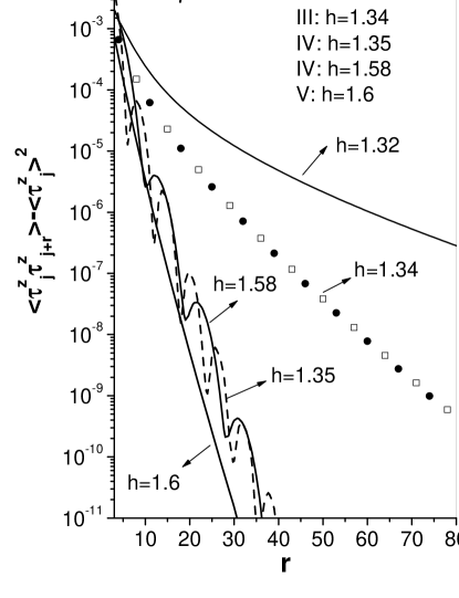
Figure 9: Static correlation function in the field direction, at $T=0,$ for $n=4,$ $\mu_{1}=\mu_{2}=\mu_{3}=\mu_{4}=1$ and for $J_{1}=1,$ $J_{2}=1.5,$ $J_{3}=1.75,$ $J_{4}=2$, as function of $r$ (distance between cells) for values of the field belonging to different regions shown in Fig. 8, where the vertical scale is decimal logarithmic.

Figure 10: Asymptotic behaviour of the direct static correlation function in the field direction, at $T=0,$ for $n=4,$ $\mu_{1}=\mu_{2}=\mu_{3}=\mu_{4}=1$ and for $J_{1}=1,$ $J_{2}=1.5,$ $J_{3}=1.75,$ $J_{4}=2$, as function of $r$ (distance between cells) for values of the field belonging to the critical lines (a), where the scales are decimal logarithmic, and disorder lines (b), where the vertical scale is also decimal logarithmic.

As in the homogenous model barouch:1971 , the asymptotic behaviour of the static correlation $\left\langle\tau_{l}^{z}(0)\tau_{l+r}^{z}(0)\right\rangle$, at $T=0$, as a function of $r,$ can be oscillatory or monotonic depending on the values of the interaction parameters. For arbitrary $n$, these regions are separated by hypersurfaces in the parameter space and are called disordered surfaces, which collapse into disorder lines for identical $\gamma^{\prime}s$. For $n=4,$ these disorder lines and the critical lines are shown in Fig.(8). Independently of the number of sites in unit cell, in the plane $\gamma\times h,$ the disorder lines are given by equation

$$h^{2}+\gamma^{2}h_{jc}^{2}=h_{jc}^{2},$$ (45)

where $h_{jc}$ is a critical field. Along these curves the anisotropic model is equivalent to an effective isotropic model barouch:1971 . For $n=2$, this equivalence is shown in Appendix A, and for $n>2$ it has been verified numerically. It is also shown, that, along this curve, the effective isotropic model is in a disordered state, which corresponds to the magnetization plateaus for the case where we have identical $\mu^{\prime}$s.

The asymptotic behaviour of the static correlation function, also for $n=4$ and at $T=0,$ as a function of the distance $r$ between cells, is presented in Fig.(9) for various values of $h$ and $\gamma$ in the different regions shown in Fig.(8). As can be seen, the behaviour, as expected alternates between oscillatory and monotonic.

At the critical point, as in the homogeneous case, the direct static correlation behaves asymptotically as $r^{-2}$barouch:1971 . This behaviour is shown in Fig.(10a), for $n=4$, and different critical fields. However, at the disorder line, differently from the homogeneous model where the direct static correlation is zero, it behaves asymptotically as $\lambda^{-r},$ where $\lambda$ is a function of the field and of the interaction parameters, as shown in Fig.(10b), for identical $\gamma^{\prime}s$ and different values of the field.

The real and imaginary parts of the dynamic correlation for a chain with $n=4$ and uniform $\mu^{\prime}s,$ at $T=0,$ are presented in Fig.(11) for values of the field greater and equal to the critical field. As in the isotropic case, apart from the asymptotic behaviour, no noticeable difference is observed in the dynamic correlation at different values of the field.

VI Dynamic Susceptibility

From the dynamic correlation $\left\langle\tau_{l}^{z}(t)\tau_{l+r}^{z}(0)\right\rangle,$ eqs.(41), we can obtain the time Fourier transform of dynamic correlation $\left\langle\tau_{l}^{z}\tau_{l+r}^{z}\right\rangle_{\omega}$ from the equation

$$\left\langle\tau_{l}^{z}\tau_{l+r}^{z}\right\rangle_{\omega}=\frac{1}{2\pi}{\displaystyle\int\limits_{-\infty}^{\infty}}\left\langle\tau_{l}^{z}(t)\tau_{l+r}^{z}(0)\right\rangle e^{i\omega t}dt,$$ (46)

which is given by

$$\left\langle\tau_{l}^{z}\tau_{l+r}^{z}\right\rangle_{\omega} =\delta(\omega)\left\langle\tau_{l}^{z}\right\rangle^{2}+$$

$$+\frac{1}{4n^{2}N^{2}}\sum_{q,k,m}\sum_{q^{\prime},k^{\prime},m^{\prime}}\mu_{m}\mu_{m^{\prime}}e^{-i(q-q^{\prime})dr}\psi_{q,k,m}\psi_{q,k,m^{\prime}}^{\ast}\phi_{q^{\prime},k^{\prime},m^{\prime}}\phi_{q^{\prime},k^{\prime},m}^{\ast}\times$$

$$\times\left[\delta\left(\omega+E_{q,k}+E_{q^{\prime},k^{\prime}}\right)n_{q,k}n_{q^{\prime},k^{\prime}}\right.+\left.\delta\left(\omega-E_{q,k}-E_{q^{\prime},k^{\prime}}\right)\left(1-n_{q,k}\right)\left(1-n_{q^{\prime},k^{\prime}}\right)\right.+$$

$$+\left.\delta\left(\omega+E_{q,k}-E_{q^{\prime},k^{\prime}}\right)n_{q,k}\left(1-n_{q^{\prime},k^{\prime}}\right)\right.+\left.\delta\left(\omega-E_{q,k}+E_{q^{\prime},k^{\prime}}\right)\left(1-n_{q,k}\right)n_{q^{\prime},k^{\prime}}\right]-$$

$$-\frac{1}{4n^{2}N^{2}}\sum_{q,k,m}\sum_{q^{\prime},k^{\prime},m^{\prime}}\mu_{m}\mu_{m^{\prime}}e^{-i(q-q^{\prime})dr}\psi_{q,k,m}\phi_{q,k,m^{\prime}}^{\ast}\psi_{q^{\prime},k^{\prime},m^{\prime}}\phi_{q^{\prime},k^{\prime},m}^{\ast}\times$$

$$\times\left[\delta\left(\omega+E_{q,k}+E_{q^{\prime},k^{\prime}}\right)n_{q,k}n_{q^{\prime},k^{\prime}}+\delta\left(\omega-E_{q,k}-E_{q^{\prime},k^{\prime}}\right)\left(1-n_{q,k}\right)\left(1-n_{q^{\prime},k^{\prime}}\right)-\right.$$

$$- \left.\delta\left(\omega+E_{q,k}-E_{q^{\prime},k^{\prime}}\right)n_{q,k}\left(1-n_{q^{\prime},k^{\prime}}\right)-\delta\left(\omega-E_{q,k}+E_{q^{\prime},k^{\prime}}\right)\left(1-n_{q,k}\right)n_{q^{\prime},k^{\prime}}\right].$$ (47)

By introducing the spatial Fourier transform

$$\left\langle\tau_{q}^{z}\tau_{-q}^{z}\right\rangle_{\omega}={\displaystyle\sum\limits_{r}}\left\langle\tau_{l}^{z}\tau_{l+r}^{z}\right\rangle_{\omega}e^{idrq},$$ (48)

in the previous expression, we can write immediately

$$\left\langle\tau_{q}^{z}\tau_{-q}^{z}\right\rangle_{\omega} =N\delta_{q,0}\delta(\omega)\left\langle\tau_{l}^{z}\right\rangle^{2}+$$

$$+\frac{1}{4n^{2}N}\sum_{q^{\prime},k,m,k^{\prime},m^{\prime}}\mu_{m}\mu_{m^{\prime}}\psi_{q^{\prime},k,m}\psi_{q^{\prime},k,m^{\prime}}^{\ast}\phi_{q^{\prime}-q,k^{\prime},m^{\prime}}\phi_{q^{\prime}-q,k^{\prime},m}^{\ast}\times$$

$$\times\left[\delta\left(\omega+E_{q^{\prime},k}+E_{q^{\prime}-q,k^{\prime}}\right)n_{q^{\prime},k}n_{q^{\prime}-q,k^{\prime}}\right.+\left.\delta\left(\omega-E_{q^{\prime},k}-E_{q^{\prime}-q,k^{\prime}}\right)\left(1-n_{q^{\prime},k}\right)\left(1-n_{q^{\prime}-q,k^{\prime}}\right)\right.+$$

$$+\left.\delta\left(\omega+E_{q^{\prime},k}-E_{q^{\prime}-q,k^{\prime}}\right)n_{q^{\prime},k}\left(1-n_{q^{\prime}-q,k^{\prime}}\right)\right.+\left.\delta\left(\omega-E_{q^{\prime},k}+E_{q^{\prime}-q,k^{\prime}}\right)\left(1-n_{q^{\prime},k}\right)n_{q^{\prime}-q,k^{\prime}}\right]-$$

$$-\frac{1}{4n^{2}N}\sum_{q^{\prime},k,m,k^{\prime},m^{\prime}}\mu_{m}\mu_{m^{\prime}}\psi_{q^{\prime},k,m}\phi_{q^{\prime},k,m^{\prime}}^{\ast}\psi_{q^{\prime}-q,k^{\prime},m^{\prime}}\phi_{q^{\prime}-q,k^{\prime},m}^{\ast}\times$$

$$\times\left[\delta\left(\omega+E_{q^{\prime},k}+E_{q^{\prime}-q,k^{\prime}}\right)n_{q^{\prime},k}n_{q^{\prime}-q,k^{\prime}}\right.+\left.\delta\left(\omega-E_{q^{\prime},k}-E_{q-q^{\prime},k^{\prime}}\right)\left(1-n_{q^{\prime},k}\right)\left(1-n_{q-q^{\prime},k^{\prime}}\right)\right.-$$

$$-\left.\delta\left(\omega+E_{q^{\prime},k}-E_{q^{\prime}-q,k^{\prime}}\right)n_{q^{\prime},k}\left(1-n_{q^{\prime}-q,k^{\prime}}\right)\right.-\left.\delta\left(\omega-E_{q^{\prime},k}+E_{q^{\prime}-q,k^{\prime}}\right)\left(1-n_{q^{\prime},k}\right)n_{q^{\prime}-q,k^{\prime}}\right].$$ (49)

The dynamic susceptibility $\chi_{q}^{zz}(\omega)$ can be obtained by using the expression zubarev:1960

$$\chi_{q}^{zz}(\omega)=-{\displaystyle\int\limits_{\infty}^{\infty}}\frac{(1-e^{-\omega^{\prime}/k_{B}T})\left\langle\tau_{q}^{z}\tau_{-q}^{z}\right\rangle_{\omega^{\prime}}d\omega^{\prime}}{\omega-\omega^{\prime}},$$ (50)

and from this we obtain

$$\chi_{q}^{zz}(\omega) =-\frac{1}{4n^{2}N}\sum_{q^{\prime},k,m,k^{\prime},m^{\prime}}\mu_{m}\mu_{m^{\prime}}\left(P_{q^{\prime},k,m,q^{\prime}-q,k^{\prime},m^{\prime}}-Q_{q^{\prime},k,m,q^{\prime}-q,k^{\prime},m^{\prime}}\right)\times$$

$$\times\left(\frac{1}{\omega+E_{q^{\prime},k}+E_{q^{\prime}-q,k^{\prime}}}-\frac{1}{\omega-E_{q^{\prime},k}-E_{q^{\prime}-q,k^{\prime}}}\right)\times\left[n_{q^{\prime},k}+n_{q^{\prime}-q,k^{\prime}}-1\right]-$$

$$-\frac{1}{4n^{2}N}\sum_{q^{\prime},k,m,k^{\prime},m^{\prime}}\mu_{m}\mu_{m^{\prime}}\left(P_{q^{\prime},k,m,q^{\prime}-q,k^{\prime},m^{\prime}}+Q_{q^{\prime},k,m,q^{\prime}-q,k^{\prime},m^{\prime}}\right)\times$$

$$\times\left(\frac{1}{\omega+E_{q^{\prime},k}-E_{q^{\prime}-q,k^{\prime}}}-\frac{1}{\omega-E_{q^{\prime},k}+E_{q^{\prime}-q,k^{\prime}}}\right)\times\left[n_{q^{\prime},k}-n_{q^{\prime}-q,k^{\prime}}\right],$$ (51)

where

$$P_{q^{\prime},k,m,q^{\prime}-q,k^{\prime},m^{\prime}} =\psi_{q^{\prime},k,m}\psi_{q^{\prime},k,m^{\prime}}^{\ast}\phi_{q^{\prime}-q,k^{\prime},m^{\prime}}\phi_{q^{\prime}-q,,k^{\prime},m}^{\ast},$$ (52)

$$Q_{q^{\prime},k,m,q^{\prime}-q,k^{\prime},m^{\prime}} =\psi_{q^{\prime},k,m}\phi_{q^{\prime},k,m^{\prime}}^{\ast}\psi_{q^{\prime}-q,k^{\prime},m^{\prime}}\phi_{q^{\prime}-q,k^{\prime},m}^{\ast},$$ (53)

and we have used the identity

$$1-n_{q,k}=e^{\beta E_{q,k}}n_{q,k}.$$ (54)

It should be noted that the previous result reduces to the known one for the isotropic modeldelima:2006 .

The static susceptibility $\chi_{q}^{zz}(0)$ is obtained by making $\omega=0$ in eq.(51), and is given by

$$\chi_{q}^{zz}(0) =-\frac{1}{2n^{2}N}\sum_{q^{\prime},k,m,k^{\prime},m^{\prime}}\mu_{m}\mu_{m^{\prime}}\left(P_{q^{\prime},k,m,q^{\prime}-q,k^{\prime},m^{\prime}}-Q_{q^{\prime},k,m,q^{\prime}-q,k^{\prime},m^{\prime}}\right)\times$$

$$\times\left(\frac{1}{E_{q^{\prime},k}+E_{q^{\prime}-q,k^{\prime}}}\right)\times\left[n_{q^{\prime},k}+n_{q^{\prime}-q,k^{\prime}}-1\right]-$$

$$-\frac{1}{2n^{2}N^{2}}\sum_{q^{\prime},k,m,k^{\prime},m^{\prime}}\left(P_{q^{\prime},k,m,q^{\prime}-q,k^{\prime},m^{\prime}}+Q_{q^{\prime},k,m,q^{\prime}-q,k^{\prime},m^{\prime}}\right)\times$$

$$\times\left(\frac{1}{E_{q^{\prime},k}-E_{q^{\prime}-q,k^{\prime}}}\right)\times\left[n_{q^{\prime},k}-n_{q^{\prime}-q,k^{\prime}}\right].$$ (55)

The isothermal susceptibility can also be obtained by using the dynamic correlation given in eq.(41), and can be written asMarshall:1971

$$\chi_{T}^{zz}={\displaystyle\sum\limits_{r}}{\displaystyle\int\limits_{0}^{\beta}}\left(\left\langle\tau_{l}^{z}(-i\lambda)\tau_{l+r}^{z}(0)\right\rangle-\left\langle\tau_{l}^{z}\right\rangle^{2}\right)d\lambda,$$ (56)

where, as defined previously, $\beta=1/k_{B}T.$ From this it can be shown that the isothermal susceptibility in the field direction is equal to the uniform static one $\chi_{0}^{zz}(0)$.

At $T=0$, the dynamic and static susceptibilities given in eqs.(51) and (55) can be explicitly written as

$$\chi_{q}^{zz}(\omega) =\frac{1}{4n^{2}N}\sum_{q^{\prime},k,m,k^{\prime},m^{\prime}}\mu_{m}\mu_{m^{\prime}}\left(P_{q^{\prime},k,m,q^{\prime}-q,k^{\prime},m^{\prime}}-Q_{q^{\prime},k,m,q^{\prime}-q,k^{\prime},m^{\prime}}\right)\times$$ (57)

$$\times\left(\frac{1}{\omega+E_{q^{\prime},k}+E_{q^{\prime}-q,k^{\prime}}}-\frac{1}{\omega-E_{q^{\prime},k}-E_{q^{\prime}-q,k^{\prime}}}\right),$$ (58)

and

$$\chi_{q}^{zz}(0) =\frac{1}{2n^{2}N}\sum_{q^{\prime},k,m,k^{\prime},m^{\prime}}\mu_{m}\mu_{m^{\prime}}\left(P_{q^{\prime},k,m,q^{\prime}-q,k^{\prime},m^{\prime}}-Q_{q^{\prime},k,m,q^{\prime}-q,k^{\prime},m^{\prime}}\right)\times$$

$$\times\left(\frac{1}{E_{q^{\prime},k}+E_{q^{\prime}-q,k^{\prime}}}\right).$$ (59)

The static susceptibility $\chi_{q}^{zz}(0),$ at $T=0$ and for $n=4,$ as a function of the field is presented in Fig.(12). For $q=0,$ as expected, it diverges at the critical fields and it tends to zero as $h\rightarrow\infty$, which corresponds to the saturation of the model. However, for $q\neq 0$ differently from the isotropic model, no divergence is present, even for a wave-vector at the zone boundary.

The real and imaginary parts of $\chi_{q}^{zz}(\omega)$ are obtained by considering $\chi_{q}^{zz}(\omega-i\epsilon)$ in the limit $\epsilon\rightarrow 0$ in   eqs.(51) and (55). The results, at $T=0$ and for $n=4,$ are shown in Fig. (13) for different wave-vectors, as functions of $\omega.$ As expected, since the Hamiltonian of the model preserves the symmetry of the spin interactions of the homogeneous one, the divergences in the real part, for any wave-vector, correspond to square-root singularities in the imaginary part.

Figure 11: (a) The real and (b) imaginary parts of the dynamic correlation function $\left\langle\tau_{l}^{z}(t)\tau_{l+1}^{z}(0)\right\rangle,$ at $T=0$ for $n=4,$ $\mu_{1}=\mu_{2}=\mu_{3}=\mu_{4}=1$ and $J_{1}=1,$ $J_{2}=1.5,$ $J_{3}=1.75,$ $J_{4}=2,$ as function of time $t.$

Figure 12: Static susceptibility in the field direction, $\chi_{q}^{zz}(0),$ at $T=0,$ as a function of the field for $n=4$, $\mu_{1}=\mu_{2}=\mu_{3}=\mu_{4}=1,$ $J_{1}=1,$ $J_{2}=1.5,$ $J_{3}=1.75,$ $J_{4}=2\ ,\gamma=0.1$ and different values of $q.$

Figure 13: (a) The real and (b) imaginary parts of the dynamic susceptibility $\chi_{q}^{zz}(\omega),$ at $T=0,$ for $n=4,$ $\mu_{1}=\mu_{2}=\mu_{3}=\mu_{4}=1,$ $J_{1}=1,$ $J_{2}=1.5,$ $J_{3}=1.75,$ $J_{4}=2,h=0.5$ and $\gamma=0.1,$ as function of frequency $\omega$ and for different values of $q.$

VII Conclusions

In this work we have considered the anisotropic XY-model on the inhomogeneous periodic chain with $N$ cells and $n$ sites per cell. The model has been exactly solved, at arbitrary temperature, for the general case where we have $n$ different exchange constants and $n$ different magnetic moments. The number of branches of the excitation spectrum is equal to $n$, and analytical results can be found for $n\leqq 4.$ For $n=2,$ explicit expressions are presented for the excitation spectrum, and, for $n=8,$ it is obtained numerically.

The induced  magnetization $M^{z}$ and the isothermal susceptibility $\chi_{T}^{zz}$ are also given by explicit expressions at arbitrary temperature. At $T=0$, where the quantum transitions induced by the tranverse field occur, the spontaneous magnetization $M^{x}$ is written in terms of the asymptotic behaviour of the determinant of a Toeplitz matrix which corresponds to the static two-spin correlation in the $x$ direction, at large separation. The critical behaviour is determined, in high numerical accuracy, by adjusting the numerical results obtained for finite Toeplitz matrices by using a non-linear regression of the scaling relation and the $\varepsilon-$algorithm. This is a rather remarkable result since it allows us to determine very precisely the critical behaviour of the system within a numerical approach. As expected, we have shown from these results that the inhomogeneous model belongs to the same universality class of the homogeneous one.

For $n$ greater than one, the system can present multiple phase transitions and it is shown that the divergence of the isothermal susceptibility $\chi_{T}^{zz},$ which is associated to inflection points in the induced magnetization, is also a signature of the quantum transitions. These critical points, as usual, correspond to the the points where the spontaneous magnetization, which is the order parameter characterizing the quantum transition, goes to zero.

Explicit results are presented for $n=4$ and $n=5,$ where we show that, differently from the isotropic model where we always have $n$ transitions, the number of quantum transitions is dependent on the values of the anisotropy parameters $\gamma.$ We have also concluded that, for $n$ even, there are two critical $\gamma^{\prime}s$, whereas, for $n$ odd, there just one critical $\gamma$ equal to zero, and this constitutes the main effect of the cell size on the critical quantum behaviour of the anisotropic model.

It has also been shown that the static two-spin correlation in the $z$ direction, as in the homogeneous model, can present oscillatory or monotonic behaviour depending on the values of $\gamma^{\prime}s$ and the field. The limiting surfaces, in the parameter space, which separates the two regimes, are the so-called disorder surfaces. For the special case when we have different $J^{\prime}s$ and identical $\gamma$’$s,$ the disorder surfaces collapse into disorder lines and, in this case, they have been determine analytically. In particular, for $n=2$, it has been proved exactly that these lines corresponds to regions where the model can be mapped onto an equivalent isotropic model. It should be noted that along the disorder lines the direct static correlation $\left\langle\tau_{l}^{z}(0)\tau_{l+r}^{z}(0)\right\rangle-\left\langle\tau_{l}^{z}\right\rangle^{2}$ presents an exponential asymptotic behaviour, differently from the homogeneous model where it is equal to zero.

We have also obtained the static and dynamic correlation on the field directions and, from these results, we have determined the dynamic wave-vector dependent susceptibility $\chi_{q}^{zz}(\omega).$ Finally, we have shown that, as in the homogeneous model, the static suceptibility $\chi_{0}^{zz}(0)$ is equal to the isothermal one $\chi_{T}^{zz}.$

VIII Acknowledgements

The authors would like thank the Brazilian agencies CNPq, Capes and Finep for partial financial support, and Dr. A. P. Vieira for enlightening discussions. L. L. Gonçalves would like to thank  Prof. S. R. A. Salinas for his hospitality during his stay, on a sabbatical leave, at the Departamento de Física Geral, Instituto de Física, Universidade de São Paulo, when this work was initiated.

IX Appendix

In this appendix we present analitycally the mapping of the anisotropic model onto the isotropic one, for a given set of parameters, for a chain with $n=2$. This mapping will be obtained, as in the homogeneous model barouch:1971 , by imposing that the isotropic and the anisotropic models have the same spectrum. As it will be shown, this equivalence is only possible when $\gamma_{1}=\gamma_{2}.$

Therefore, let us consider the matrices $\mathbb{A}_{q}$ and$\mathbb{\ B}_{q},$ given by eqs.(14) and (15), which in this case are explicitly given by

$$\mathbb{A}_{q}=-\left(\begin{array}[c]{cc}\mu_{1}h&\frac{J_{1}}{2}+\frac{J_{2}}{2}\exp(-i2q)\\ \frac{J_{1}}{2}+\frac{J_{2}}{2}\exp(i2q)&\mu_{2}h\end{array}\right),$$ (60)

$$\mathbb{B}_{q}=-\left(\begin{array}[c]{cc}0&\frac{J_{1}\gamma_{1}}{2}-\frac{J_{2}\gamma_{2}}{2}\exp(-i2q)\\ -\frac{J_{1}\gamma_{1}}{2}+\frac{J_{2}\gamma_{2}}{2}\exp(i2q)&0\end{array}\right).$$ (61)

From these results we obtain the matrix $\left(\mathbb{A}_{q}+\mathbb{B}_{q}\right)\left(\mathbb{A}_{q}-\mathbb{B}_{q}\right),$ whose eigenvalues, determined from eq.(17), which constitute the two branches of the spectrum of the chain which are given by

$$E_{q,k=1,2}^{2} =\frac{1}{2}\left[\alpha_{1}+\alpha_{2}+\left(c_{1}+c_{2}\right)\cos 2q\right]\pm\frac{1}{2}\left\{\left[\alpha_{1}+\alpha_{2}+\left(c_{1}+c_{2}\right)\cos 2q\right]^{2}\right.-$$

$$-\left.4\left[\left(\alpha_{1}+c_{1}\cos 2q\right)\left(\alpha_{2}+c_{2}\cos 2q\right)-\beta^{2}-\delta^{2}-2\beta\delta\cos 2q\right]\right\}^{1/2},$$ (62)

where

$$\alpha_{1} \equiv\mu_{1}^{2}h^{2}+a_{1}^{2}+b_{2}^{2};\text{ }\alpha_{2}\equiv\mu_{2}^{2}h^{2}+a_{2}^{2}+b_{1}^{2},$$

$$a_{1} \equiv\frac{J_{1}}{2}\left(1+\gamma_{1}\right);\text{ \ }a_{2}\equiv\frac{J_{2}}{2}\left(1+\gamma_{2}\right),$$

$$b_{1} \equiv\frac{J_{1}}{2}\left(1-\gamma_{1}\right);\text{ \ }b_{2}\equiv\frac{J_{2}}{2}\left(1-\gamma_{2}\right),$$

$$c_{1} \equiv\frac{J_{1}J_{2}}{2}\left(1+\gamma_{1}\right)\left(1-\gamma_{2}\right)\text{; \ }c_{2}\equiv\frac{J_{1}J_{2}}{2}\left(1-\gamma_{1}\right)\left(1+\gamma_{2}\right),$$

$$\beta \equiv(\mu_{1}b_{1}+\mu_{2}a_{1})h;\text{ \ }\delta\equiv(\mu_{1}a_{2}+\mu_{2}b_{2})h.$$ (63)

From the previous result we can obtain the spectrum of the isotropic chain, with parameters $\mu_{1}^{\prime}h^{{}^{\prime}}$, $\mu_{2}^{\prime}h^{{}^{\prime}}$, $J_{1}^{{}^{\prime}},$ $J_{2}^{{}^{\prime}},$ by making  $\gamma_{1}=\gamma_{2}=0$ and from this we can write

$$\varepsilon_{q,k=1,2} =\frac{1}{2}\left[(\mu_{1}^{\prime 2}+\mu_{2}^{\prime 2})h^{{}^{\prime}2}+\frac{J_{1}^{{}^{\prime}2}}{2}+\frac{J_{2}^{{}^{\prime}2}}{2}+J_{1}^{{}^{\prime}}J_{2}^{{}^{\prime}}\cos 2q\right]\pm$$

$$\pm\frac{1}{2}\left(\mu_{1}^{\prime}+\mu_{2}^{\prime}\right)h^{{}^{\prime}}\sqrt{\left(\mu_{1}^{\prime}-\mu_{2}^{\prime}\right)^{2}h^{{}^{\prime}2}+J_{1}^{{}^{\prime}2}+J_{2}^{{}^{\prime}2}+2J_{1}^{{}^{\prime}}J_{2}^{{}^{\prime}}\cos 2q}.$$ (64)

By imposing the equivalence of the two spectra we conclude immediately that we should have $c_{1}=c_{2}\equiv c$, which implies that $\gamma_{1}=\gamma_{2}\equiv\gamma.$ Introducing these conditions in eq.(62) we obtain

$$E_{q,k=1,2}^{2}=\frac{1}{2}\left[\alpha_{1}+\alpha_{2}+2c\cos 2q\right]\pm\frac{1}{2}\sqrt{\left(\alpha_{1}-\alpha_{2}\right)^{2}+4\left(\beta^{2}+\delta^{2}\right)+8\beta\delta\cos 2q,}$$ (65)

and by comparing it with eq.(64) we can write immediately the mapping relations

$$(\mu_{1}^{\prime 2}+\mu_{2}^{\prime 2})h^{{}^{\prime}2}+\frac{J_{1}^{{}^{\prime}2}}{2}+\frac{J_{2}^{{}^{\prime}2}}{2}=(\mu_{1}^{2}+\mu_{2}^{2})h^{2}+\frac{\left(J_{1}^{2}+J_{2}^{2}\right)}{2}\left(1+\gamma^{2}\right),$$ (66)

$$J_{1}^{{}^{\prime}}J_{2}^{{}^{\prime}}=J_{1}J_{2}\left(1-\gamma^{2}\right),$$ (67)

$$\left(\mu_{1}^{\prime 2}-\mu_{2}^{\prime 2}\right)^{2}h^{{}^{\prime}4}+h^{{}^{\prime}2}\left(\mu_{1}^{\prime}+\mu_{2}^{\prime}\right)^{2}\left(J_{1}^{{}^{\prime}2}+J_{2}^{{}^{\prime}2}\right)=\left(\mu_{1}^{2}-\mu_{2}^{2}\right)^{2}h^{4}+$$

$$+\gamma^{2}\left(J_{1}^{2}-J_{2}^{2}\right)^{2}+\left(J_{1}^{2}+J_{2}^{2}\right)\left[\left(\mu_{1}+\mu_{2}\right)^{2}h^{2}-\gamma^{2}\left(\mu_{1}-\mu_{2}\right)^{2}h^{2}\right],$$ (68)

$$\left(\mu_{1}^{\prime}+\mu_{2}^{\prime}\right)^{2}h^{{}^{\prime}2}J_{1}^{{}^{\prime}}J_{2}^{{}^{\prime}}=J_{1}J_{2}\left[\left(\mu_{1}+\mu_{2}\right)^{2}h^{2}-\gamma^{2}\left(\mu_{1}-\mu_{2}\right)^{2}h^{2}\right].$$ (69)

This set of equations is not independent, and this means that the parameters of the equivalent isotropic model are not uniquely determined. Moreover, we can show that eqs.(66) to (69) can only present a solution if the parameters of the anisotropic model satisfy the equation

$$\left(J_{1}^{2}-J_{2}^{2}\right)^{2}\left(1-\gamma^{2}\right)^{2}-8\mu_{1}\mu_{2}h^{2}\left(J_{1}^{2}+J_{2}^{2}\right)\left(1-\gamma^{2}\right)+16\mu_{1}^{2}\mu_{2}^{2}h^{4}=0.$$ (70)

This expression is obtained after some lengthy but straigthforward algebra, by using the result

$$\left(\mu_{1}^{\prime}+\mu_{2}^{\prime}\right)^{2}h^{{}^{\prime}2}=\frac{\left(\mu_{1}+\mu_{2}\right)^{2}h^{2}-\gamma^{2}\left(\mu_{1}-\mu_{2}\right)^{2}h^{2}}{1-\gamma^{2}},$$ (71)

which is obtained from eqs. (66) and (69), and eqs. (66),(67) e (71). The solution of eq.(70) gives the result

$$h=\pm\frac{\left|J_{1}\pm J_{2}\right|\sqrt{1-\gamma^{2}}}{2\sqrt{\mu_{1}\mu_{2}}}\equiv\widetilde{h}_{c}\sqrt{1-\gamma^{2}}$$ (72)

where $\widetilde{h}_{c}$ are the critical fields of the anisotropic model in the limit $\gamma\longrightarrow 0.$ Although this result, for the disorder lines, is restricted to $n=2$, we have verified numerically that, for identical $\gamma^{\prime}s,$ it is still valid for arbitrary $n$. In particular, for n=4, the numerical verification of eq.(72) is shown in Fig.(8).

References

• (1) H. E. Lieb, T. Schultz and D. C. Mattis, Two soluble models of antiferromagnetic chain, Ann. Phys. 16 407 (1961).
• (2) E. Dagotto and T. M. Rice, Surprises on the way from one- to two-dimensional quantum magnets: the ladder materials, Science 271, 618 (1996).
• (3) T. N. Nguyen, P. A. Lee and H. C. Loye, Design of a random quantum spin chain paramagnet: $Sr_{3}CuPt_{0.5}Ir_{0.5}O_{6}$, Science 27, 489 (1996).
• (4) P. Gambardella, A. Dallmeyer, K. Maiti, M. C. Malagoli,W. Eberhardt, K. Kern and C. Carbone, Ferromagnetism in one-dimensional monoatomic metal chains, Nature 416, 301 (2002).
• (5) C.J. Mukherjeea, R. Coldea, D.A. Tennant, M. Kozac, M. Enderlec, K. Habichtd, P. Smeibidld, and Z. Tylczynski, Field-induced quantum phase transition in the quasi 1D XY-like antiferromagnet $Cs_{2}CoCl_{4},$ J. Magn. Magn. Matt, 272–276, 920 (2004).
• (6) M. Matsumoto, B. Normand, T. M. Rice and M. Sigrist, Field- and pressure-induced magnetic quantum phase transitions in $TlCuCl_{3},$Phys. Rev. B  69, 054423 (2004).
• (7) S. Sachdev, Quantum phase transitions (Cambridge University Press, 2000).
• (8) L. Amico, F. Baroni, A. Fubini, D. Patanè, V. Tognetti, and P. Verrucchi, Divergence of the entanglement range in low-dimensional quantum systems, Phys. Rev. A 74, 022322 (2006).
• (9) K. E. Feldman, Exact diagonalization of the XY-Hamiltonian of open linear chains with periodic coupling constants and its application, J. Phys. A: Math. Gen. 39, 1039 (2006).
• (10) P. Tong and M. Zhong, Quantum phase transitions of periodic anisotropic XY chain in a transverse field, Physica B 304, 91 (2001).
• (11) O. Derzhko, J. Richter, T. Krokhmalskii and O. Zaburannyi, Regularly alternating spin-1/2 anisotropic XY chains: The ground-state and thermodynamic properties, Phys.Rev.E 69, 066112 (2004).
• (12) P. Tong and X. Liu, Lee-Yang zeros of the partition function of periodic and quasiperiodic, Phys. Rev. Lett. 97, 017201 (2006).
• (13) J. P. de Lima, T. F. A. Alves and L. L. Gonçalves, The isotropic XY model on the inhomogeneous periodic chain, J. Magn. & Magn. Mater. 298, 95 (2006).
• (14) F. F. Barbosa Filho, J. P. de Lima and L. L. Gonçalves, The anisotropic XY model on the 1D alternating superlattice, J. Magn. & Magn. Mater. 226-230, 638 (2001).
• (15) J. P. de Lima and L. L. Gonçalves, The longitudinal dynamic correlation and dynamic susceptibility of the isotropic XY-model on the 1D alternating superlattice, Physica A 311, 458 (2002).
• (16) Th. J. Siskens, H. W. Capel and J. H. H. Perk, Antiferromagnetic chain with alternating interactions and magnetic moments, Phys.Lett. A 53, 21 (1975).
• (17) J. H. H. Perk , H. W. Capel, M. J. Zuilhof and Th. J. Siskens, On a soluble model of an antiferromagnetic chain with alternatin interactions and magnetic moments, Physica A 81, 319 (1975).
• (18) J. H. H. Perk and H. W. Capel, Time- and frequency-dependent correlation functions for the homogeneous and alternating isotropic XY-models, Physica 100A, 1 (1980).
• (19) J. H. Taylor and G. Müller, Magnetic field effects in the dynamics of alternating or anisotropic quantum spin chains, Physica A 130, 1 (1985).
• (20) L.L.Gonçalves and J.P. de Lima, The XY-model on the one-dimensional superlattice, J. Magn. & Magn. Mater. 140-144, 1606 (1995).
• (21) Th. J. Siskens and P. Mazur, Time-correlation functions in the a-ciclic XY model, Physica 71, 560 (1974).
• (22) H. W. Capel and J. H. H. Perk, Autocorrelation function of x-component of the magnetization in the one-dimensional XY-model, Physica A 87, 211 (1977).
• (23) L. L. Gonçalves, Theory of properties of some one-dimensional systems (D. Phil. Thesis, University of Oxford, 1977).
• (24) Th. Niemeijer, Some exact calculations on a chain of spin $1/2$, Physica 37, 377 (1967).
• (25) E. Barouch and B. M. McCoy, Statistical Mechanics of the XY model II: Spin-correlation functions Phys. Rev. A, 3, 786 (1971)
• (26) H.E. Stanley, Phase Transitions and Critical Phenomena (Oxford University Press, 1971)
• (27) M. N. Barber, in Phase Transitions and Critical Phenomena, Eds. J. Lebowitz and C. Domb (Academic Press, London, 1983) v. 8, p. 146.
• (28) D. N. Zubarev, Double-time Green functions in statistical physics, Sov. Phys. Usp. 3, 320 (1960).
• (29) See for instance W. Marshall and Lovesey, Theory of Thermal Neutron Scatering (Oxford University Press, Oxford, 1971), Appendix B.