Current-induced spin polarization and the spin Hall effect: a quasiclassical approach

Abstract

The quasiclassical Green function formalism is used to describe charge and spin dynamics in the presence of spin-orbit coupling. We review the results obtained for the spin Hall effect on restricted geometries. The role of boundaries is discussed in the framework of spin diffusion equations.

, , ,

1 Introduction

A transverse (say along the $y$-axis) $z$-polarized spin current flowing in response to an applied (say along the $x$-axis) electrical field

$$J^{z}_{s,y}=\sigma_{sH}E_{x},$$ (1)

is referred to as the spin Hall effect, and $\sigma_{sH}$ is called spin Hall conductivity[1, 2]. This effect allows for the generation and control of spin currents by purely electrical means, which is a great advantage when operating electronic devices. Physically, the possibility of a non-vanishing $\sigma_{sH}$ is due to the presence of spin-orbit coupling, which in semiconductors may be orders of magnitude larger than in vacuum. Clearly, two key issues are (i) how sensitive is the spin Hall conductivity to various solid state effects like disorder scattering, electron-electron interaction etc. and (ii) how the spin current can actually be detected experimentally. About the first issue, there is now a consensus that the effect of disorder scattering depends on the form of the spin-orbit coupling. In the case of the two-dimensional electron gas with a Rashba type of spin-orbit coupling, arbitrarily weak disorder leads to the vanishing of the spin Hall conductivity in the bulk limit[3, 4, 5, 6, 7, 8, 9]. Concerning the second issue, the first experimental observations[10, 11] of the spin Hall effect have been achieved by measuring, optically, the spin polarization accumulated at the lateral edges of an electrically biased wire. Hence, the understanding of the spin Hall effect involves the description of boundaries. In order to address the two issues mentioned above, we develop in the following a quasiclassical Green function approach for the description of charge and spin degrees of freedom in the presence of spin-orbit coupling.

2 The Eilenberger equation

In this section we sketch how to derive the Eilenberger equation for the quasiclassical Green function in the presence of spin-orbit interaction [12]. We consider the following Hamiltonian

$$H=\frac{p^{2}}{2m}+\mathbf{b}\cdot{\boldsymbol{\sigma}},$$ (2)

where $\textbf{b}(\mathbf{p})$ is an effective internal magnetic field due to the spin-orbit coupling. For instance, in the Rashba case we have $\mathbf{b}=\alpha\mathbf{p}\times\mathbf{{\hat{e}}}_{z}$. The Green function $\check{G}_{t_{1}t_{2}}(\textbf{x}_{1},\textbf{x}_{2})$ is a matrix both in Keldysh and spin space and obeys the Dyson equation $(\hbar=1)$

$$\left(\textrm{i}\partial_{t_{1}}+\frac{1}{2m}\partial^{2}_{\mathbf{x}_{1}}+\mu-\mathbf{b}(-\textrm{i}\partial_{\mathbf{x}_{1}})\cdot{\boldsymbol{\sigma}}\right)\check{G}_{t_{1}t_{2}}(\mathbf{x}_{1},\mathbf{x}_{2})=\delta(t_{1}-t_{2})\delta(\mathbf{x}_{1}-\mathbf{x}_{2}).$$ (3)

A quasiclassical description is possible when the Green function depends on the center-of-mass coordinate, $\mathbf{x}=(\mathbf{x}_{1}+\mathbf{x}_{2})/2$, on a much larger scale than on the relative coordinate, ${\mathbf{r}}=\mathbf{x}_{1}-\mathbf{x}_{2}$. In this situation, by going to the Wigner representation

$$\check{G}(\mathbf{x}_{1},\mathbf{x}_{2})=\sum_{\mathbf{p}}e^{\textrm{i}\mathbf{p}\cdot{\mathbf{r}}}\check{G}(\mathbf{p},\mathbf{x)}$$ (4)

and subtracting from Eq.(3) its complex conjugate, one obtains a homogeneous equation for $\check{G}(\mathbf{p},\mathbf{x})$

$$\textrm{i}\partial_{t}\check{G}+\frac{\textrm{i}}{2}\big{\{}\frac{\mathbf{p}}{m}+\frac{1}{2}\partial_{\mathbf{p}}(\mathbf{b}\cdot{\boldsymbol{\sigma}}),\partial_{\mathbf{x}}\check{G}\big{\}}-\left[\mathbf{b}\cdot{\boldsymbol{\sigma}},\check{G}\right]=\left[\Sigma,\check{G}\right],$$ (5)

where only the center-of-mass time, $t=(t_{1}+t_{2})/2$, appears. On the right-hand-side of Eq.(5) we have also introduced the self-energy

$$\Sigma=\frac{1}{2\pi N_{0}\tau}\sum_{\mathbf{p}}\check{G}(\mathbf{p},\mathbf{x}),$$ (6)

which takes into account disorder scattering at the level of the self-consistent Born approximation. In the spirit of the quasiclassical approximation, we make the following ansatz for $\check{G}$

$$\check{G}=\left(\begin{array}[]{cc}G^{R}&G^{K}\\ 0&G^{A}\end{array}\right)=\frac{1}{2}\left\{\left(\begin{array}[]{cc}G_{0}^{R}&0\\ 0&-G_{0}^{A}\end{array}\right),\left(\begin{array}[]{cc}\tilde{g}^{R}&\tilde{g}^{K}\\ 0&\tilde{g}^{A}\end{array}\right)\right\},$$ (7)

where we assume that $\tilde{g}$ does not depend on the modulus of $\mathbf{p}$ but at most on its direction. In this way we have separated the fast variation of the free Green function in the relative coordinate $\mathbf{r}$ from the slow variation of $\tilde{g}$ in the center-of-mass coordinate $\mathbf{x}$. The quasiclassical Green function is defined as

$$\check{g}(\mathbf{\hat{p}},\mathbf{x})\equiv\frac{i}{\pi}\int_{-\infty}^{\infty}\mathrm{d}\xi\ \check{G}(\mathbf{p},\mathbf{x}),$$ (8)

where $\xi=p^{2}/2m-\mu$ and $\mathbf{\hat{p}}=\mathbf{p}/p$. Using the ansatz above, the $\xi$-integration can be done explicitly. By assuming that $\mathbf{b}=b(p)\mathbf{\hat{b}}(\mathbf{\hat{p}})$ and

$$G_{0}^{R}=\sum_{\nu=\pm}\frac{\textbf{P}_{\nu}}{\epsilon-\xi-\nu b(\xi)+\mathrm{i}0^{+}},\ \ \textbf{P}_{\pm}=\frac{1}{2}\left(1\pm\hat{\textbf{b}}\cdot{\boldsymbol{\sigma}}\right)$$ (9)

we find

$$\frac{i}{\pi}\int_{-\infty}^{\infty}\mathrm{d}\xi\ G_{0}^{R}=\frac{N_{+}}{N_{0}}\textbf{P}_{+}+\frac{N_{-}}{N_{0}}\textbf{P}_{-}\equiv g_{0}^{R},$$ (10)

where $N_{+}$ and $N_{-}$ are the densities of state of the spin-split bands. In the absence of spin-orbit coupling, $N_{\pm}=N_{0}$, and the function $\tilde{g}$ coincides with the $\xi$-integrated Green function $\check{g}$. In the present case, however,

$$\check{g}=\frac{1}{2}\{g_{0}^{R},\tilde{g}\}.$$ (11)

By inverting Eq.(11) one has

$$\tilde{g}=\frac{1}{2}\{(g_{0}^{R})^{-1},g\}+\frac{1}{4}\left[(g_{0}^{R})^{-1},\left[g_{0}^{R},g\right]\right]\approx\frac{1}{2}\left\{\left(1-\frac{N_{+}-N_{-}}{2N_{0}}\hat{\textbf{b}}\cdot{\boldsymbol{\sigma}}\right),\check{g}\right\},$$ (12)

where the last approximation, to be used in the following, holds for $b\ll\epsilon_{F}$. The $\xi$-integration of $\check{G}$ multiplied by a momentum dependent function leads to

$$\frac{i}{\pi}\int_{-\infty}^{\infty}\mathrm{d}\xi\ m(\textbf{p})\check{G}=\frac{1}{2}\{\textbf{M}g_{0}^{R},\tilde{g}\}.$$ (13)

where $\textbf{M}=m(\textbf{p}_{+})\textbf{P}_{+}+m(\textbf{p}_{-})\textbf{P}_{-}$, and ${\bf p}_{\pm}$ are the Fermi momenta in the two bands. To first order in $b/\epsilon_{F}$ one obtains

$$\frac{1}{2}\{\mathbf{M}g_{0}^{R},\tilde{g}\}\approx\frac{1}{2}\{\mathbf{M},\check{g}\}=m(\textbf{p}_{+})\check{g}_{+}+m(\textbf{p}_{-})\check{g}_{-},$$ (14)

where $\check{g}_{\pm}=\frac{1}{2}\{P_{\pm},\check{g}\}$. Hence the standard procedure to obtain the Eilenberger equation for $\check{g}$ via the $\xi$-integration of Eq.(5) yields

$$\sum_{\nu=\pm}\big{(}\partial_{t}\check{g}_{\nu}+\frac{1}{2}\left\{\frac{\bf p_{\nu}}{m}+\frac{\partial}{\partial\bf p}({\bf b}_{\nu}\cdot{\boldsymbol{\sigma}}),\frac{\partial}{\partial{\bf x}}\check{g}_{\nu}\right\}+{\rm i}[{\bf b}_{\nu}\cdot{\boldsymbol{\sigma}},\check{g}_{\nu}]\big{)}=-{\rm i}\left[\check{\Sigma},\check{g}\right].$$ (15)

Eq.(15) holds even for internal fields $\mathbf{b}$ for which the factorization $\mathbf{b}=b(p)\mathbf{\hat{b}}(\mathbf{\hat{p}})$ is not possible, as long as one can assume $|\mathbf{b}|\ll\epsilon_{F}$. For more details see [12].

From the above Eilenberger equation the expression for the charge and spin currents are readily obtained, since the Fermi surface average $\langle\ldots\rangle$ of Eq.(15) has the form of a continuity equation

$$\partial_{t}\langle\check{g}_{c}\rangle+\partial_{\bf x}\cdot\check{\bf J}_{c} = 0$$ (16)

$$\partial_{t}\langle\check{g}_{x}\rangle+\partial_{\bf x}\cdot\check{\bf J}_{s}^{x} = 2\sum_{\nu=\pm}\langle{\bf b}_{\nu}\times{\bf\check{g}_{\nu}}\rangle_{x}$$ (17)

$$\partial_{t}\langle\check{g}_{y}\rangle+\partial_{\bf x}\cdot\check{\bf J}_{s}^{y} = 2\sum_{\nu=\pm}\langle{\bf b}_{\nu}\times{\bf\check{g}_{\nu}}\rangle_{y}$$ (18)

$$\partial_{t}\langle\check{g}_{z}\rangle+\partial_{\bf x}\cdot\check{\bf J}_{s}^{z} = 2\sum_{\nu=\pm}\langle{\bf b}_{\nu}\times{\bf\check{g}_{\nu}}\rangle_{z},$$ (19)

where we expanded the Green function in charge and spin components, $\check{g}=\check{g}_{c}+\check{\bf g}\cdot{\boldsymbol{\sigma}}$. For instance, the spin current with spin polarization along the $\mathbf{e}_{z}$ axis reads

$${\bf j}_{s}^{z}({\bf x},t)=-\frac{N_{0}}{4}\int{\rm d}\epsilon\,[{\bf{\check{J}}}_{s}^{z}(\epsilon;{\bf x},t)]^{K},$$ (20)

with ${\check{\bf J}}_{s}^{z}(\epsilon;{\bf x},t)=\langle{\bf v}_{F}{\check{g}}_{z}\rangle$.

3 Spin Hall effect

Before considering explicitly the role of the boundaries, it is useful to see how the spin Hall effect in the bulk may be analyzed in the present formalism. For a stationary and space independent case the equation for the Keldysh component can be written in the following way ($a=2\alpha p_{F}\tau$)

$$\left(\begin{array}[]{cccc}1&0&0&0\\ 0&1&0&a\hat{p}_{x}\\ 0&0&1&a\hat{p}_{y}\\ 0&-a\hat{p}_{x}&-a\hat{p}_{y}&1\end{array}\right)\left(\begin{array}[]{c}g_{c}^{K}\\ g_{x}^{K}\\ g_{y}^{K}\\ g_{z}^{K}\end{array}\right)=\left(\begin{array}[]{cccc}1&-{\alpha}\hat{p}_{y}/v_{F}&{\alpha}\hat{p}_{x}/v_{F}&0\\ -{\alpha}\hat{p}_{y}/v_{F}&1&0&0\\ {\alpha}\hat{p}_{x}/v_{F}&0&1&0\\ 0&0&0&1\end{array}\right)\left(\begin{array}[]{c}\langle g_{c}^{K}\rangle\\ \langle g_{x}^{K}\rangle\\ \langle g_{y}^{K}\rangle\\ \langle g_{z}^{K}\rangle\end{array}\right)+S_{E}.$$ (21)

In the above we have introduced the mean free path $l=v_{F}\tau$. The presence of the electric field, along the $\mathbf{{\hat{e}}}_{x}$ axis, is accounted for by the source term $S_{E}$

$$S_{E}=-4|e|Elf^{\prime}(\epsilon)\left[\left(\begin{array}[]{c}\hat{p}_{x}\\ 0\\ 0\\ 0\\ \end{array}\right)+\frac{\alpha}{v_{F}}\left(\begin{array}[]{c}0\\ -2\hat{p}_{x}\hat{p}_{y}\\ \hat{p}_{x}^{2}-\hat{p}_{y}^{2}\\ 0\\ \end{array}\right)\right],$$ (22)

which has been introduced in the Eilenberger equation by exploiting the gauge invariance in the derivative terms. In the above $f(\epsilon)$ is the Fermi function. Notice that spin-charge coupling effects arise at the order of $\alpha/v_{F}$. From the angular average of Eq.(21) one observes immediately that $\langle{\hat{p}}_{x}g_{z}^{K}\rangle=\langle{\hat{p}}_{y}g_{z}^{K}\rangle=0$, i.e. no spin current with polarization along ${\bf{\hat{e}}}_{z}$ flows in the system. It is also instructive to first express $g^{K}_{z}$ in terms of the angle-averaged quantity $\langle g^{K}\rangle$ and then multiply by $p_{y}$ and take the angular average. The spin current reads then

$$j_{y}^{z}=\frac{v_{F}\alpha p_{F}\tau}{1+(2\alpha p_{F}\tau)^{2}}\left(\alpha|e|\tau N_{0}E+s_{y}\right).$$ (23)

When comparing to a calculation of the spin-Hall conductivity within the standard Kubo-formula approach, one realizes that the first term in square brackets corresponds to the simple bubble diagram, while the second term accounts for vertex corrections due to the spin-dependent part of the velocity operator. This second term is related to a voltage induced spin polarization in ${\bf{\hat{e}}}_{y}$ direction that was first obtained by Edelstein [13], $s_{y}=-|e|\alpha\tau N_{0}E$.

In summary, we find that under the very special conditions we considered here the spin-Hall current is zero. We started from the Rashba Hamiltonian, that has a linear-in-momentum spin orbit coupling, we assumed that elastic scattering is spin-conserving, and finally we considered the stationary solution in the bulk of the two-dimensional electron system so that the spin density neither depends on space nor time. Relaxing one or more of these conditions finite spin-Hall currents are expected.

4 Boundary conditions and diffusion equation

The derivation of the boundary conditions for the quasiclassical Green function is a delicate task, due to the fact that the boundary potential typically varies on a microscopic length scale which is shorter than the quasiclassical resolution. Therefore one must include the boundary effect in the very process of the derivation of the Eilenberger equation. This is especially important for interfaces between two different materials, where transport occurs through a tunnel junction or a point contact. Often a boundary with vacuum is simpler to describe since one couples only one incoming with one outgoing channel. In the presence of spin-orbit coupling, the non-conservation of spin and in particular the beam splitting, i.e., one incoming channel with direction ${\bf p}_{in}$ can be scattered into two outgoing channels ${\bf p}_{out}$, makes the problem more difficult and there is not yet a complete derivation of boundary conditions for the quasiclassical Green function.

In the following we limit to two special types of boundary conditions and discuss their role as far as spin relaxation and the spin Hall effect are concerned[14]. The first type of boundary conditions requires spin conservation, i.e. the spin currents normal to the interface are zero. We refer to them in the following as hard-wall boundary conditions, (see also [15, 16]). For smooth confining potential it has been pointed out, that specular scattering involves some spin rotation in such a way to keep the scattered particle in the eigenstate of the incoming one [17]. We refer to this situation as soft-wall boundary conditions.

The matching condition for the quasiclassical Green function can be obtained following the approach of Ref. [18] and reads

$$\check{g}(\mathbf{\hat{p}}_{out})=S\check{g}(\mathbf{\hat{p}}_{in})S^{{\dagger}},$$ (24)

where the matrix $S$ describes the scattering at the boundary.

To illustrate the role of boundaries, we consider the diffusive limit where a detailed analytical treatment is possible and which is also relevant for actual experiments.

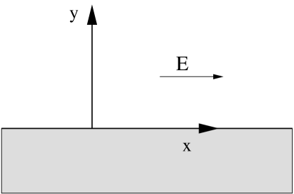
Figure 1: Orientation of the boundary and the electric field.

We assume that our two-dimensional electron gas is limited to the half-space $y>0$ and that there is a uniform electric field along the $\mathbf{\hat{e}}_{x}$ direction, see Fig. 1. Since the system is translational invariant along the $\mathbf{\hat{e}}_{x}$ direction, we consider only space dependence with respect to the $\mathbf{\hat{e}}_{y}$ direction. The diffusion equation reads

$$\left(\partial_{t}-D\partial_{y}^{2}\right)\rho = 2B\partial_{y}s_{x}$$ (25)

$$\left(\partial_{t}-D\partial_{y}^{2}\right)s_{x} = -\frac{1}{\tau_{s}}s_{x}+2B\partial_{y}\rho$$ (26)

$$\left(\partial_{t}-D\partial_{y}^{2}\right)s_{y} = -\frac{1}{\tau_{s}}(s_{y}-s_{0})+2C\partial_{y}s_{z}$$ (27)

$$\left(\partial_{t}-D\partial_{y}^{2}\right)s_{z} = -\frac{2}{\tau_{s}}s_{z}-2C\partial_{y}s_{y},$$ (28)

with $D=\frac{1}{2}v_{F}^{2}\tau$, $\tau_{s}=\tau/[2(\alpha p_{F}\tau)^{2}]$, $B=4\alpha^{3}p_{F}^{2}\tau^{2}$, $C=v_{F}\alpha p_{F}\tau$, and $s_{0}=-|e|\alpha\tau N_{0}E$ is the bulk spin polarization in the presence of an electric field, mentioned at the end of the previous section. A general solution of the diffusion equations (25-28) can be found in the form

$$s(y,t)=e^{-\gamma t}e^{\textrm{i}qy}\left(\begin{array}[]{c}\rho\\ s_{x}\\ s_{y}\\ s_{z}\end{array}\right),$$ (29)

where a static solution requires $\gamma=0$. In the absence of electric field (i.e., $s_{0}=0$), as in optical spin excitation experiments, the solution with longest lifetime has a finite wave vector in contrast to standard diffusion. The presence of boundaries does affect this result. With hard-wall boundary conditions

$$-D\partial_{y}s_{x}={\bf n}\cdot{\bf j}_{x} = 0,$$ (30)

$$-D\partial_{y}s_{y}-Cs_{z}={\bf n}\cdot{\bf j}_{y} = 0,$$ (31)

$$-D\partial_{y}s_{z}+C(s_{y}-s_{0})={\bf n}\cdot{\bf j}_{z} = 0,$$ (32)

where ${\bf n}$ is in the $y$-direction, the mode with longest lifetime is localized at the boundary. With soft-wall boundary conditions, one has

$$s_{x}=0\,\,\text{and}\,\,s_{y}=s_{0},$$ (33)

while the $z$-component of the spin is still conserved and therefore Eq. (32) remains valid. Due to the decoupling, at the boundary, of the three spin components, the mode with longest lifetime is no longer confined to the boundary and has $s_{x}\propto\sin(qy)$, $s_{y}-s_{0}\propto\sin(qy)$, $s_{z}\propto\cos(qy)$ with $q\sim L_{s}^{-1}$ (as in the bulk), where $L_{s}=\sqrt{D\tau_{s}}$ is the spin diffusion length. Although the two types of boundary conditions have a different effect in a time-dependent optical spin-relaxation experiment, both imply that, in the absence of an electrical field, the only static solution of the diffusion equation is with vanishing polarization (See Ref.[14] for further details).

The presence of an electric field does not change this result provided the polarization in the $\mathbf{\hat{e}}_{y}$ direction is replaced by the difference $s_{y}-s_{0}$, which enters both the diffusion equations (25-28) and the boundary conditions (30-33). Hence, in the presence of an electric field, the only static solution has $s_{y}=s_{0}$, $s_{x}=0$ and $s_{z}=0$. Furthermore, the second condition in (33) means that, with soft-wall boundary conditions and at the level of diffusive accuracy, the time-dependent approach to the static solution becomes infinitely fast at the boundary, in contrast to what happens in the bulk where relaxation occurs in a finite time.

5 Numerical results

In this section we give a brief overview of numerical results for both spin Hall effect and spin accumulation in finite systems. In the following we consider the Rashba Hamiltonian on a rectangular strip of length $L_{x}$ and width $L_{y}$ which is connected to reservoirs at $x=0$ and $x=L_{x}$. We impose soft-wall boundary conditions at $y=0$ and $y=L_{y}$. At $t=0$ the electrical field $E$ is applied in $x-$direction. In order to solve the time-dependent Eilenberger equation (15) numerically we introduce the discretization $\Delta x$ and $\Delta t$ for space and time, respectively. Our algorithm is exact to order $(\Delta t)^{2}$ and $(\Delta x)^{4}$ and yields stable solutions for arbitrary long times provided $\Delta t$ is chosen small enough. The boundary conditions are imposed such that at the border for incoming momenta the Green function is calculated from the Eilenberger equation while for outgoing momenta the scattering condition Eq.(24) is applied.

Figure 2: Voltage induced spin polarization as function of $y$ and $t$ at $x=L_{x}/2$ on a strip of length $L_{x}=20\,l$ and width $L_{y}=10\,l$ for $\alpha/v_{F}=10^{-3}$. The upper figures are obtained for $\alpha p_{F}\tau=1$, whereas in the lower figures $\alpha p_{F}\tau=0.1$. Left panel: $s_{y}$, right panel: $s_{z}$, both in units of the bulk polarization $s_{0}$.

Fig. 2 shows the time evolution of the spin polarization on a line across the strip at $x=L_{x}/2$, the Rashba parameter is $\alpha/v_{F}=10^{-3}$. In the upper part of the figure the elastic scattering rate $\tau$ is chosen such that $\alpha p_{F}\tau=1$ which is already beyond the reach of the diffusion equation approach. The $y-$component $s_{y}$ of the spin polarization (left panel) increases monotonically from zero to the bulk value $s_{0}$ while $s_{z}$ (right panel) shows strong oscillations close to the boundaries which decay after a few periods. These oscillations are associated with a spin current polarized in $z-$direction and flowing in $y-$direction. The magnitude of this spin current corresponds to a spin Hall conductivity $\sigma_{sH}\simeq e/8\pi$ which however persists only on a short time scale after switching on the electrical field. In the stationary limit only the bulk polarization of $s_{y}$ survives while the polarization of $s_{x}$ and $s_{z}$ is restricted to a small region around the corners of the strip[3, 12]. In addition, the shape of these corner polarizations depends strongly on the details of the coupling between the reservoirs and the strip. In the lower part of Fig. 2 we choose $\alpha p_{F}\tau=0.1$, i.e. the spin dynamics is diffusive. Note that at the boundaries $s_{y}$ approaches $s_{0}$ on a much shorter time scale than in the bulk, in accordance with the boundary condition (33). Due to the overdamped dynamics of the spins there are neither in $s_{y}$ nor in $s_{z}$ time dependent oscillations.

To summarize, the quasiclassical approach provides a versatile theoretical framework for the description of the coherent spin dynamics in confined electron systems in the presence of spin-orbit coupling.

This work was supported by the Deutsche Forschungsgemeinschaft through Sonderforschungsbereich 484.

References

- [1] S. Murakami, N. Nagaosa, and S.-C. Zhang, Science 301, 1348 (2003).
- [2] J. Sinova, D. Culcer, Q. Niu, N. A. Sinitsyn, T. Jungwirth, and A. H. MacDonald, Phys. Rev. Lett. 92, 126603 (2004).
- [3] E. G. Mishchenko, A. V. Shytov, and B. I. Halperin, Phys. Rev. Lett. 93, 226602 (2004).
- [4] J. I. Inoue, G. E. W. Bauer, and L. W. Molenkamp, Phys. Rev. B 70, 041303(R) (2004).
- [5] R. Raimondi and P. Schwab, Phys. Rev. B 71, 033311 (2005).
- [6] O. V. Dimitrova, Phys. Rev. B 71, 245327 (2005).
- [7] O. Chalaev and D. Loss, Phys. Rev. B 71, 245318 (2005).
- [8] S. Murakami, Phys. Rev. B 69, 241202(R) (2004).
- [9] A. Khaetskii, Phys. Rev. Lett. 96, 056602 (2006).
- [10] Y. K. Kato, R. C. Myers, A. C. Gossard, and D. D. Awschalom, Science 306, 1910 (2004).
- [11] J. Wunderlich, B. Kaestner, J. Sinova, and T. Jungwirth, Phys. Rev. Lett. 94, 047204 (2005).
- [12] R. Raimondi, C. Gorini, P. Schwab, and M. Dzierzawa, Phys. Rev. B 74, 035340 (2006).
- [13] V. M. Edelstein, Solid State Commun. 73, 233 (1990); J. Phys.: Condens. Matter 5, 2603 (1993).
- [14] P. Schwab, M. Dzierzawa, C. Gorini, and R. Raimondi, Phys. Rev. B 74, 155316 (2006).
- [15] V. M. Galitski, A. A. Burkov, and S. Das Sarma, Phys. Rev. B 74, 115331 (2006).
- [16] O. Bleibaum, Phys. Rev. B 74, 113309 (2006).
- [17] A. O. Govorov, A. V. Kalameitsev, and J. P. Dulka, Phys. Rev. B 70, 245310 (2004).
- [18] A. Millis, D. Rainer, and J. A. Sauls, Phys. Rev. B 38, 4504 (1988).