A time-dependent density functional theory scheme for efficient calculations of dynamic (hyper)polarizabilities

Abstract

We present an efficient perturbative method to obtain both static and dynamic polarizabilities and hyperpolarizabilities of complex electronic systems. This approach is based on the solution of a frequency dependent Sternheimer equation, within the formalism of time-dependent density functional theory, and allows the calculation of the response both in resonance and out of resonance. Furthermore, the excellent scaling with the number of atoms opens the way to the investigation of response properties of very large molecular systems. To demonstrate the capabilities of this method, we implemented it in a real-space (basis-set free) code, and applied it to benchmark molecules, namely CO, H₂O, and paranitroaniline (PNA). Our results are in agreement with experimental and previous theoretical studies, and fully validate our approach.

I Introduction

The optical properties of a material are essentially determined by the response of the electrons to an external field. If this applied field is small, the induced dipole of the system can be expanded in powers of the fieldbutcher ; bloembergen . The first order coefficient is the so-called electric polarizability $\alpha$. This quantity describes, e.g., the dielectric properties of the material and how light is absorbed and emitted. In second order we obtain the first hyperpolarizability $\beta$, that is responsible for the processes of second-harmonic generation, optical rectification and Pockles effectbutcher . Higher order terms can be related to other electro-optical effects like third-harmonic generation, the Kerr effect, etc. Finally, polarizabilities are called static or dynamic if the perturbing field is static or frequency dependent.

The importance of the linear term, $\alpha$, is well known in Physics and Chemistrybonin . On the other hand, non-linear (i.e. beyond first order) optical effects have gained quite some interest lately due to their technological applications in opto-electronic devices. Nonlinear optical materials can be used to convert light to shorter (bluer) wavelengths, which can be focused to a smaller spot size. Shorter wavelength light sources would hence yield higher density optical recording media (such as DVDs and CDs). Other applications include tunable light sources, image recognition systems and adaptive optics.

Several methods have been used to calculate (hyper)polarizabilities of finite systemslanghoff ; shelton94 ; bishop ; review_baroni ; cardoso . In the static case, the simplest approach is finite differences gready77 that uses the definition of the polarizabilities as derivatives of the dipole (or of the total energy) with respect to the applied field. Calculations are performed at various (small) field strengths, and the required derivatives are evaluated numerically. This method is simple and straightforward to implement. However, it requires many total energy evaluations, and these need to have a very high precision to obtain reasonable numerical derivatives. Moreover, it is not possible to generalize this idea to the dynamic case.

Another widely used approach is perturbation theory, of which more than one flavor exists. In the sum-over-states method langhoff ; orr71 the (hyper)polarizabilities are written as an infinite sum over occupied and empty states, that involves the ground-state eigenvalues and dipole matrix elements. In a similar vein, one can obtain the polarizabilities from the corresponding response functions written in the product basis of occupied and empty states or in terms of Green’s functionssenatore8910 . Note that these techniques can be used both for static and dynamic response. Although widely used by the community, these methods have several shortcomings. First, results are often difficult to converge with the number (and quality) of the empty states. Second, the scaling with the number of atoms is quite unfavorable, making hard the application to the study of large system, like nanostructures or molecules with biological interest.

A different technique also used to obtain both static and dynamic linear polarizabilities is the direct solution of the time-dependent Schrödinger equation in real time Yabana96 . In this way only the occupied subspace is needed and the scaling with system size is excellent [${\cal O}(N^{2})$, where $N$ is the number of atoms]. However, this method cannot be easily generalized to extract hyperpolarizabilities.

A very interesting approach that essentially solves the problems mentioned above is the Sternheimer equationsternheimer . Although a perturbative technique, it avoids the use of empty states, and has a quite good scaling with the number of atoms. This method has already been used for the calculation of many response propertiesreview_baroni like atomic vibrations (phonons), electron-phonon coupling, magnetic response, etc. In the domain of optical response, this method has been mainly used for static response, although a few first principles calculations for low frequency (far from resonance) (hyper)polarizabilities have appearedsenatore87 ; karna90a ; vangisbergen97 ; bertsch01 . Recently, a reformulation of the Sternheimer equation in a super operator formalism was presentedbaroni_turbo . When combined with a Lanczos solver, it allows to calculate very efficiently the first order polarizability for the whole frequency spectrum. However the generalization of this method to higher orders is not straight-forward.

In this Article, we propose a modified version of the Sternheimer equation that is able to cope with both static and dynamic response in and out of resonance. The solution of the first-order Sternheimer equation gives us access to both $\alpha$ and $\beta$. Higher order polarizabilities can be obtained from an hierarchy of Sternheimer equations. Exchange and correlation effects are treated at the level of density functional theory (DFT)hk for static polarizabilities and time-dependent DFT (TDDFT)tddft for the dynamic case. Compared to other quantum-chemistry approaches, density functional methods have a somewhat lower accuracy but are lighter numerically, allowing the study of much larger systems. In the present work we focus on finite systems but the method has also been applied to periodic systems for the non-resonant caserubio96 . Note that in the field of DFT, the Sternheimer equation is often referred to as density functional perturbation theory review_baroni .

The rest of this Article is organized as follows. In Sect. II we present the derivation of the frequency-dependent Sternheimer equation and show how to obtain the linear polarizability and first hyperpolarizability from its solution. In the following section we give some details concerning the implementation of our method. In Sect. IV we apply this theory to several test molecules, comparing our results to other calculations and experiments. Finally we present our conclusions and a brief outlook.

II Theory

II.1 Linear Response

Within TDDFT, the quantum state of an interacting electronic system is described by the time-dependent Kohn-Sham equations (atomic units will be used unless explicitly stated)

$$i\frac{\partial}{\partial{t}}\psi_{m}({\bm{r}},t)=H_{\rm KS}\left(t\right)\psi_{m}({\bm{r}},t)\,.$$ (1)

The Kohn-Sham Hamiltonian is written as

$$H_{\rm KS}=-\frac{\nabla^{2}}{2}+v_{\rm ext}({\bm{r}},t)+v_{\rm Hartree}({\bm{r}},t)+v_{\rm xc}({\bm{r}},t)\,,$$ (2)

where the first term corresponds to the kinetic energy, and the following ones represent the external potential, the Hartree potential that describes the classical interaction between the electrons, and the exchange-correlation term that accounts for all non-trivial parts of the electron-electron interaction. Note that the Hartree and exchange-correlation terms are time-dependent as they are functionals of the (time-dependent) density. This latter quantity can be evaluated from the occupied Kohn-Sham orbitals

$$n({\bm{r}},t)=\sum_{m}^{\rm occ.}|\psi_{m}({\bm{r}},t)|^{2}\,.$$ (3)

We are concerned with external potentials that are the sum of a time-independent part, typically created by a set of nuclei, and a monochromatic electric field $v_{\rm field}({\bm{r}},t)=\sum_{i=1}^{3}\lambda_{i}\,r_{i}\cos\left(\omega{t}\right)$. If we assume that the magnitude of $\lambda$ is small, we can use perturbation theory to expand the Kohn-Sham wave-functions in powers of $\lambda$. The first order term reads

$$\psi_{m}({\bm{r}},t)=e^{-i\left(\epsilon_{m}+\sum_{i=1}^{3}\lambda_{i}\epsilon^{(1)}_{m\,i}\right){t}}\Big{\{}\psi^{(0)}_{m}({\bm{r}})+\\ \frac{1}{2}\sum_{i=1}^{3}\big{[}\lambda_{i}e^{i\omega{t}}\psi^{(1)}_{m,\,i}({\bm{r}},\omega)+\lambda_{i}{e^{-i\omega{t}}}\psi^{(1)}_{m,\,i}({\bm{r}},-\omega)\big{]}\Big{\}}\,,$$ (4)

where $\psi^{(0)}_{m}({\bm{r}})$ are the wave functions of the static Kohn-Sham Hamiltonian $H^{(0)}$ obtained by taking $\lambda=0$

$$H^{(0)}\psi^{(0)}_{m}({\bm{r}})=\epsilon_{m}\psi^{(0)}_{m}({\bm{r}})\,,$$ (5)

and $\psi^{(1)}_{m,\,i}({\bm{r}},\omega)$ are the first order variations of the time-dependent Kohn-Sham wave-functions.

From (4) and the definition of the time-dependent density Eq. (3), we can obtain the time dependent density

$$n\left({\bm{r}},t\right)=n^{\left(0\right)}\left({\bm{r}}\right)+\frac{1}{2}\sum_{i=1}^{3}\big{[}\lambda_{i}e^{i\omega{t}}n^{(1)}_{i}({\bm{r}},\omega)\\ +\lambda_{i}{e^{-i\omega{t}}}n^{(1)}_{i}({\bm{r}},-\omega)\big{]}\Big{\}}\,,$$ (6)

with the definition of the first-order variation of the density

$$n^{\left(1\right)}_{i}({\bm{r}},\omega)=\sum_{m}^{\rm occ.}\Big{\{}\left[\psi^{\left(0\right)}_{m}\left({\bm{r}}\right)\right]^{*}\psi^{\left(1\right)}_{m,\,i}({\bm{r}},\omega)\\ +\left[\psi^{\left(1\right)}_{m,\,i}({\bm{r}},-\omega)\right]^{*}\psi^{\left(0\right)}_{m}\left({\bm{r}}\right)\Big{\}}\ .$$ (7)

By replacing the expansion of the wave-functions (4) in the time-dependent Kohn-Sham equation (1), and picking up the first order terms in $\lambda$, we arrive at a Sternheimer equation for the variations of the wave functions

$$\left\{H^{\left(0\right)}-\epsilon_{m}\pm\omega+i\eta\right\}\psi^{\left(1\right)}_{m,\,i}({\bm{r}},\pm\omega)=\\ -P_{c}H^{\left(1\right)}_{i}(\pm\omega)\psi_{m}^{\left(0\right)}({\bm{r}})\,,$$ (8)

with the first order variation of the Kohn-Sham Hamiltonian

$$H^{\left(1\right)}_{i}(\omega)=r_{i}+\int\!{\rm d}^{3}r^{\prime}\,\frac{n^{\left(1\right)}({\bm{r}}^{\prime},\omega)}{|{\bm{r}}-{\bm{r}}^{\prime}|}\\ +\int\!{\rm d}^{3}r^{\prime}\,f_{\rm xc}({\bm{r}},{\bm{r}}^{\prime})\,n^{\left(1\right)}({\bm{r}^{\prime}},\omega)\,,$$ (9)

where $P_{c}$ is the projector onto the unoccupied subspace. The effect of this projector is to make zero the components of $\psi^{\left(1\right)}_{m,\,i}({\bm{r}},\pm\omega)$ in the subspace of the occupied ground state wavefunctions. In linear response, these components do not contribute to the variation of the density, therefore we can safely ignore the projector. This is important for large systems as the cost of the calculation of the projections scales quadratically with the number of orbitals.

The first term of $H^{\left(1\right)}_{i}(\omega)$ comes from the external perturbative field, while the next two represent the variation of the Hartree and exchange-correlation potentials. The exchange-correlation kernel is a functional of the ground-state density $n^{\left(0\right)}$, and is given by the functional derivative

$$f_{\rm xc}[n^{\left(0\right)}]({\bm{r}},{\bm{r}}^{\prime})=\left.\frac{\delta v_{\rm xc}({\bm{r}})}{\delta n({\bm{r}}^{\prime})}\right|_{n=n^{\left(0\right)}}\,.$$ (10)

In the previous equations we made use of the adiabatic approximation to write $f_{\rm xc}$ as a frequency independent quantity. Equations (7) and (8) form a set of self consistent equations for linear response, that only depend on the occupied ground state orbitals.

Note that we included in Eq. (8) a positive infinitesimal $\eta$. This term is essential to obtain the correct position of the poles of the causal response function, and therefore to obtain the imaginary part of the polarizability. Furthermore, using a small, but finite, $\eta$ allows us to solve numerically the Sternheimer equation close to resonances, as it removes the divergences of this equation.

By following the same kind of reasoning, we can arrive at a hierarchy of Sternheimer equations for the higher order terms in $\lambda$. These will be needed for the calculation of $\gamma$, the second order hyperpolarizability, or higher order hyperpolarizabilitiesgonze95 .

II.2 Polarizability

The time dependent dipole moment is defined as

$$\mu_{i}(t)=\int\!{\rm d}^{3}r\,n\left({\bm{r}},t\right)r_{i}\,.$$ (11)

The polarizabilities are defined by the expansion of the dipole moment in terms of the electric field

$$\mu_{i}(t)=\mu_{i}(0)+\sum_{j}^{3}\alpha_{ij}(\omega_{j})\lambda_{j}\cos(\omega_{j}t)\\ +\frac{1}{2!}\sum_{j,k=1}^{3}\beta_{ijk}(-\omega_{j}-\omega_{k};\omega_{j},\omega_{k})\lambda_{j}\lambda_{k}\cos(\omega_{j}t)\cos(\omega_{k}t)\\ +\ldots$$ (12)

We must notice that there are several conventions for the definition of the (hyper)polarizabilities, which are conveniently detailed in Ref. willetts92, . In this work we follow convention AB (where the prefactors $1/n!$ are explicitly included in Eq. 12), that appears to be the most used by the theoretical community. All referenced values have been converted to this convention.

If we replace expression (7) in Eq. (11) and compare with (12) we can obtain a formula for the polarizability in terms of the variation of the density

$$\alpha_{ij}(\omega)=\int\!{\rm d}^{3}r\,n^{\left(1\right)}_{j}({\bm{r}},\omega)r_{i}\,.$$ (13)

The quantity most easily accessible experimentally is the photoabsorption cross section, that can be evaluated directly from the linear polarizability

$$\bar{\sigma}(\omega)=\frac{4\pi\omega}{c}\mathfrak{Im}\,\bar{\alpha}(\omega)\,,$$ (14)

where $\bar{\alpha}$ is the trace of the polarizability tensor

$$\bar{\alpha}(\omega)=\frac{1}{3}\sum_{i=1}^{3}\alpha_{ii}(\omega)\ .$$ (15)

II.3 First hyperpolarizability

If for the dynamic hyperpolarizabilities we follow the same procedure as before, we get an expression in terms of the second order variation of the density that requires the evaluation of higher order variations of the wave functions. However, it is possible to get the first hyperpolarizability directly from the first order variations by means of the $2n+1$ theorem. This theorem states that the $n$th order variations of the wave functions are enough to obtain the $2n+1$ derivative of the energygonze89 ; review_baroni . This theorem can be expanded to the dynamic case and allows us to write the first hyperpolarizability $\beta$ in terms of the first order variations of the wave functions. After some algebra, we arrive atrubio96

$$\beta_{ijk}(-\omega_{1};\omega_{2},\omega_{3})=-4\sum_{P}\sum_{\zeta=\pm 1}\Bigg{\{}\sum_{m}^{occ.}\int\!{\rm d}^{3}r\,\psi^{(1)*}_{m,\,i}({\bm{r}},-\zeta\omega_{1})H^{\left(1\right)}_{j}(\zeta\omega_{2})\psi^{\left(1\right)}_{m,\,k}({\bm{r}},\zeta\omega_{3})\\ -\sum_{mn}^{occ.}\int\!{\rm d}^{3}r\,\psi^{(0)*}_{m}({\bm{r}})H^{\left(1\right)}_{j}(\zeta\omega_{2})\psi^{(0)}_{n}({\bm{r}})\int\!{\rm d}^{3}r\,\psi^{(1)*}_{n,\,i}({\bm{r}},-\zeta\omega_{1})\psi^{(1)}_{m,\,k}({\bm{r}},\zeta\omega_{3})\\ -\frac{2}{3}\int\!{\rm d}^{3}r\,\!\!\!\int\!{\rm d}^{3}r^{\prime}\,\!\!\!\int\!{\rm d}^{3}r^{\prime\prime}\,K_{\rm xc}({\bm{r}},{\bm{r}}^{\prime},{\bm{r}}^{\prime\prime})n^{\left(1\right)}_{i}({\bm{r}},\omega_{1})n^{\left(1\right)}_{j}({\bm{r}}^{\prime},\omega_{2})n^{\left(1\right)}_{k}({\bm{r}}^{\prime\prime},\omega_{3})\Bigg{\}}\ .$$ (16)

where the first sum is over the permutations $P$ of the pairs $(i,-\omega_{1})$, $(j,\omega_{2})$, and $(k,\omega_{3})$ and the exchange-correlation kernel, written in the adiabatic approximation, reads

$$K_{\rm xc}({\bm{r}},{\bm{r}}^{\prime},{\bm{r}}^{\prime\prime})=\left.\frac{\delta^{2}v_{\rm xc}({\bm{r}})}{\delta n({\bm{r}}^{\prime})\delta n({\bm{r}}^{\prime\prime})}\right|_{n=n^{(0)}}\,.$$ (17)

The first hyperpolarizability tensor has 27 components and is in general non-symmetric. The quantity that is experimentally relevant is

$$\beta_{\parallel}=\frac{1}{5}\sum_{i=1}^{3}\left(\beta_{zii}+\beta_{izi}+\beta_{iiz}\right)$$ (18)

Where $z$ is oriented in the direction of the dipole moment of molecule. Sometimes the equivalent quantity $\beta_{\rm vec}=\beta_{z}=5/3\,\beta_{\parallel}$ is used.

III Implementation

This scheme has been implemented using a real space grid-based formulation in the code octopusoctopus03 . We have chosen a real space grid, as it allows us a systematic convergence of the results (hyperpolarizabilities are notoriously difficult to converge with localized basis sets). However, uniform grids can not easily describe all-electron atoms, so we replace the electron-nuclear Coulomb interaction by Kleinman-Bylander pseudopotentials. This is, however, a well controlled approximation for the systems we are interested in.

In (TD)DFT several approximations exist for the exchange-correlation term Scuseria05 . In our approach we can treat the exchange-correlation term at two levels, one is the ground state exchange-correlation potential involved in the calculation of the ground state wave functions, and the other is the exchange-correlation kernel. For the ground state, except were noted otherwise, we use the local density approximation (LDA), we will also use the exact exchange functional in the KLIKLI approximation. For the exchange-correlation kernel, we have decided to use, due to its simplicity, the adiabatic local density approximation (LDA). (Although our scheme is quite general and can in principle be applied to any exchange-correlation functional.)

The LDA is a well studied approximation, and is quite reliable in the prediction of many properties. One important main defect in this context is the wrong asymptotic part of the LDA exchange-correlation potential, that for neutral systems decays exponentially instead of falling as $1/r$. This usually leads to small HOMO-LUMO gaps which implies systems that are too polarizable, in contrast to Hartree-Fock where the gap is larger and the magnitudes of the polarizabilities are underestimated. The exchange and correlation kernel will contribute to reduce the independent particle polarizability even at ALDA level (this contribution for extended systems is zero and as the long range behavior of the XC potential is not relevant in this regime, this clearly points that the non-locality of the XC kernel as well as self-interaction correction are responsible for the bad performance of LDA). We will observe this overestimation in the calculations that follow. In fact, in the case of compact finite systems there has been indications that the exchange-correlation potential seems to be more important than the kernelStener2001 . The situation is particularly problematic in the case of long molecular chains5.4.vanGisbergen , where standard exchange-correlation functionals can greatly overestimate polarizabilities when compared to many-body approaches. Note, however, that this is not a deficiency of DFT, but of the LDA approximation (and of many exchange-correlation functionals), that can in principle be treatedCasida00 by using more sophisticated orbital dependent functionals like the self-interaction corrected LDA ldapz or the exact exchangegoerling94 . However in present orbital functionals there is still a significant correlation contribution that is not taken into account and is responsible for the discrepancies between theory and experiment for long-chains in the exact exchange approach5.4.vanGisbergen .

Numerically, the central part of our scheme is the solution of the Sternheimer equation (8). This has the form of a linear equation were the operator to invert is the shifted ground state Hamiltonian. As the shift is complex (due to the $i\eta$ term), this operator is not Hermitian. Therefore, we can not use standard techniques common in the community, like the simple conjugated gradients scheme, but have to rely on more general (and involved) linear solvers. Our choice was the biconjugate gradient stabilized methodSaad . Close to the resonance frequencies, the Sternheimer equation becomes very badly conditioned, and the solution process turns out to be very costly. The problem can be eased by the use of preconditioning. We have found that a smoothing preconditionersaad96 can dramatically improve convergence in these cases. Also for small system the solution process can be made less costly if we solve the Sternheimer equation in the space of the unoccupied wave functions by orthogonalizing the right-hand side of the Sternheimer equation with respect to the occupied wave functions. Although this would not be practical for large systems as the orthogonalization process can become very demanding.Even with these techniques, the process is much more costly for frequencies near resonance. For example, for the CO case, the full self-consistent solution of the Sternheimer equation for a single frequency in a single direction requires around $1700$ applications of the Hamiltonian, for the a near resonance frequency approximately 10 times more applications are required. As a comparison, for the ground state DFT calculation around $2000$ Hamiltonian operations are needed.

As the right-hand side of the Sternheimer equation depends on the linear variation of the density, the problem has to be solved self-consistently. For this, we use similar strategies as for the ground-state calculation, mixing the linear variation of the density using a Broyden schemeBroyden65 in order to speed up the convergence of the self-consistent cycle.

The Poisson equation is solved using the interpolating scaling functions scheme proposed in Ref. isf, . As this process has to be done only once per self-consistency iteration, the performance of the Poisson solver is not critical.

The total cost of calculating the response is of order ${\cal O}(N_{ks}N_{g}M_{\omega})$, where $N_{ks}$ is the number of Kohn-Sham orbitals, $N_{g}$ is the number of grid points and $M_{\omega}$ is the number of frequencies we desire (which is independent of the system size). This scaling is much better than for the approaches that relay on expansions in particle-hole states, and even better than for the ground-state calculation that normally scales as ${\cal O}(N_{ks}N^{2}_{g})$ (due to the necessity of orthogonalizing the wave-functions). We believe, therefore, that this method can be used to study (hyper)polarizabilities of very large systems, like nanostructures or molecules with biological interest. After obtaining the linear response, the evaluation of the hyperpolarizability from Eq. (16) has a cost proportional to ${\cal O}(N^{2}_{ks}N_{g}M_{\omega})$ but with a very small prefactor. Note that ${\cal O}(N)$ (with $N$ the number of atoms) schemes are available for ground stateordern and static polarizability calculationsordernpol . These linear scaling methods are based on “nearsightness”kohn or the idea of divide and conqueryang . The real space treatment used in our method would allow for the incorporation of these strategies to reduce even further the numerical cost for large systems.

IV Examples of applications

We decided to illustrate the implementation of our method by applying it to some simple molecules that have been well studied both experimentally and theoretically: CO, H₂O, and paranitroaniline (PNA).

In all our calculations we took the experimental geometries: $\overline{\rm CO}=1.13$ Å; $\overline{\rm HO}=0.957$ Å, ${\rm\hat{HOH}}=104.5^{\rm o}$; the experimental geometry of PNA determined through X-ray crystallography can be found in Ref. bertinelli77, . However, there are two CH distances missing from the crystallographic data. For these we followed Ref. salek05, and took their theoretical values (see Table 1 of Ref. karna91, ). In all cases the dipole moment of the molecule was taken perpendicular to the $z$ axis, for H₂O the molecule was considered in the $yz$ plane and in the case of PNA it was taken in the $xz$ plane. We used Troullier-Martins norm-conserving pseudopotentials with a core radius of 0.66 Å for H, 0.78 Å for C and 0.74 Å for both N and O.

We used a simulation box composed of spheres centered at each atomic position, with a radius of 9.5 Å for CO, 7.4 Å H₂O and 5.3 Å for PNA. The points were distributed in a regular grid with spacing 0.20 Å for CO, 0.17 Å for H₂O, and 0.19 Å for PNA. With these parameters, hyperpolarizabilities are converged to better than 1%. As expected, the simulation boxes required to converge the hyperpolarizabilities were much larger than the ones typically used in ground-state calculations, as these quantities have sizeable contributions from the regions far away from the nuclei. The required simulation box size depends on the frequency of the perturbation, being larger for higher frequencies. Finally, we used the LDA parameterization by Perdew and Zungerldapz to approximate the exchange-correlation functionals.

	This work	LDA	HFa	MP4a	CCSD(T)a	Exp.
$\mu$	0.0631		-0.1052	0.0905	0.057	0.0481b
$\alpha_{xx}$	12.55		11.25	12.00	11.97
$\alpha_{zz}$	15.82		14.42	15.53	15.63
$\bar{\alpha}$	13.64	13.87c	12.31	13.18	13.19	13.09d
$\beta_{xxz}$	8.35	8.24e	5.0	8.3	8.4
$\beta_{zzz}$	33.34	33.52e	31.1	28.3	30.0
$\beta_{\parallel}$	30.03	30.00e	24.8	27.0	28.0

Table 1: Comparison of static polarizabilities and hyperpolarizabilities for CO. Results are in atomic units. ^aFinite differences results from Ref. hp_co, . ^bExperimental result from Ref. mu_co, . ^cLDA basis set results from Ref. vangisbergen98a, . ^dExperimental result from Ref. pol_co, . ^eLDA basis set results from Ref. vangisbergen98b, .

We will start our discussion with CO. The results for static properties are displayed in Table 1. The results fully agree with the other DFT-LDA calculations. Compared to more sophisticated quantum chemistry methods, the LDA overestimates the values for the polarizabilities and the hyperpolarizabilities. This, as mentioned before, comes from a deficiency in the asymptotic region of the LDA potential.

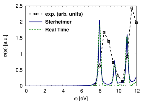
Figure 1: Average photo-absorption cross section of the CO molecule, calculated within the adiabatic LDA. The line corresponds to the results obtained through the solution of the Sternheimer equation, while the dots are obtained through the solution in real-time of the time-dependent Kohn-Sham equation. Low resolution experimental absorption cross-section from Ref. Chan93, . For a more detailed comparison, the relevant experimental excitation energies are at: 8.51 eV ($A^{1}\Pi$), 10.78 eV ($B^{1}\Sigma^{+}$), 11.40 eV ($C^{1}\Sigma^{+}$), and 11.53 eV ($E^{1}\Pi$)Chan93 ; Nielson80 .

We now turn to the dynamic properties. In Fig. 1 we plot the absorption cross section of the CO molecule obtained with our approach, and compared to the spectrum obtained through the direct solution of the time-dependent Kohn-Sham equations in real-time. As expected, the two calculations agree perfectly, which validates our numerical implementation of the Sternheimer equations. Note that, even if both methods have identical scalings, the solution of the Sternheimer equation still has a larger prefactor if the whole spectrum is required. This is due to the ill-conditioning of the linear system close to resonances. From Fig. 1 it is clear that the two theoretical results are red-shifted with respect to the experimental curve. This shortcoming of the simple LDA can be corrected by using functionals with the correct asymptotic behavior Casida00 .

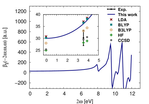
Figure 2: (Color online) Second harmonic generation $\beta_{||}(-2\omega;\omega,\omega)$ of CO. The inset shows a comparison of the results of this work (TDLDA) with other available results. Exp: Experimental results from Ref. shelton94, ; HF: Hartree Fock results from Ref. salek05, ; LDA, BLYP, B3LYP: DFT results from Ref. salek05, ; CCSD: Coupled cluster results from Ref. salek05, .

In Fig. 2 we present our calculations of the second harmonic generation spectrum, $\beta_{||}(-2\omega;\omega,\omega)$, of CO, together with the available experimental resultsshelton94 and previous theoretical datasalek05 . Our results agree very well with previous DFT results using the LDA. We can also see that the use of the generalized gradient approximation BLYP (Becke 88 Becke88 for exchange and Lee, Yang, and Parr LYP88 correlation) does not change significantly the results. Using a hybrid functional, the Becke 3 parameter B3LYP functional Becke93 , does reduce the error, while Hartree-Fock (HF) results underestimate the value for the hyperpolarizability. The best results are, as expected, obtained by coupled cluster calculations using singles and doubles (CCSD).

	$\bm{\omega}=$0.00 eV		$\bm{\omega}=$1.79 eV		$\bm{\omega}=$1.96 eV
	This work	LDAa	This work	LDAa	This work	LDAa
$\beta_{zzz}$	-21.23	-19.14	-27.67	-25.22	-29.37	-26.81
$\beta_{zxx}$	-9.84	-8.82	-12.89	-11.45	-13.68	-12.11
$\beta_{xxz}$	-9.84	-8.82	-16.87	-15.57	-19.28	-17.90
$\beta_{zyy}$	-12.08	-11.67	-14.94	-14.39	-15.68	-15.09
$\beta_{yyz}$	-12.08	-11.67	-14.48	-13.99	-15.06	-14.56

Table 2: Tensor components for second harmonic generation $\beta(-2\omega;\omega,\omega)$ of H₂O. ^aTheoretical results from Ref. salek05, .

Now we turn to the H₂O molecule. To test our implementation, we show, in Table 2, the different components of the hyperpolarizability tensor for $\omega=0$ eV, 1.79 eV, and 1.96 eV. We see that our results compare well to previous theoretical work salek05 . The small difference can be explained by the different numerical methodologies (real-space grid and pseudopotentials in our case and basis sets in Ref. salek05, ).

	$\alpha(0,0)$	$\beta_{\parallel}(0;0,0)$	$\beta_{\parallel}(0;\omega,-\omega)$	$\beta_{\parallel}(-2\omega;\omega,\omega)$
This work (TDLDA)	10.51	-25.89	-28.33	-34.71
This work (KLI/ALDA)	8.61	-11.75	-12.43	-14.03
LDAa	10.5	-26.1	-28.6	-35.1
BLYPa	10.8	-27.9	-30.9	-38.8
LB94a	9.64	-17.8	-17.7	-20.3
LDAb	10.63	-23.78	-26.09	-32.12
BLYPb	10.77	-23.65	-26.11	-32.76
B3LYPb	9.81	-18.54	-20.11	-24.11
HFb	8.53	-10.73	-11.27	-12.52
CCSD(T)c	9.79	-18.0	-19.0	-21.1
exp.	9.81d			-22$\pm$9e

Table 3: Comparison of (hyper)polarizabilities of H₂O for different DFT calculations. CCSD(T) and experimental values are given as reference. For dynamic results $\omega=1.79\ [\mbox{eV}]$. ^aGrid based calculations from Ref. bertsch01, ; ^bBasis set calculations from Ref. salek05, ; ^cResults from Ref. sekino93, ; ^dExperimental results from Ref. spackman89, ; ^eExperimental results from Ref. ward79, ;

In Table 3 we show the static polarizability, $\alpha(0,0)$, the static first hyperpolarizability, $\beta_{\parallel}(0;0,0)$, the optical rectification, $\beta_{\parallel}(0;\omega,-\omega)$, and second harmonic generation, $\beta_{\parallel}(-2\omega;\omega,\omega)$ for water. All dynamic values were calculated for $\omega=1.79$ eV. This time we also have included results with the KLI orbital dependent exchange-correlation potential combined with the ALDA exchange-correlation kernel. Concerning LDA values, we can see that our results fully agree with the results of Ref. bertsch01, that also uses a grid based representation, while basis-set results from Ref. salek05, differ by less than 10%. We can see that all LDA and BLYP values overestimate the magnitude of (hyper)polarizabilities with respect to experiment and coupled cluster calculations. The use of more sophisticated exchange correlation functionals, like LB94 or B3LYP, improves significantly the results, while the KLI/ALDA scheme gives an underestimation of the magnitude of (hyper)polarizabilities similar to Hartee-Fock results.

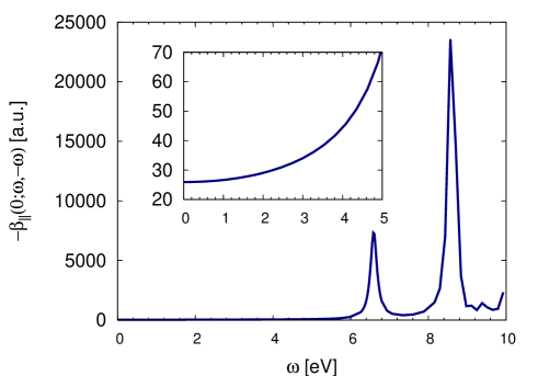
Figure 3: Calculated optical rectification $\beta_{\parallel}\left(0;\omega;-\omega\right)$ of H₂O.

To conclude the discussion of water results, we plot, in Fig. 3 the frequency dependence of the optical rectification in the visible and near ultraviolet regimes. It is clear that our method not only works for small non-resonant frequencies but also in the more complicated resonant regime.

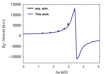
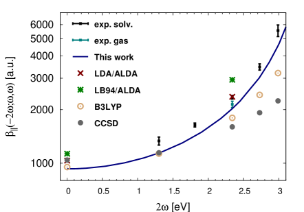
Figure 4: (Color online) Second harmonic generation $\beta_{||}(-2\omega;\omega,\omega)$ of paranitroaniline. Note that the $y$ axis in the right panel is in logarithmic scale. exp. solv.: Solvent phase experimental results from Ref. teng83, ; exp. gas: Gas phase experimental results from Ref. kaatz98, ; LDA/ALDA, LB94/ALDA: DFT basis set results from Ref. vangisbergen98b, ; B3LYP: DFT basis set results from Ref. salek02, ; CCSD: Coupled cluster results from Ref. salek05, . Some references use a different convention to define hyperpolarizabilities, all the values shown here have been converted to convention AB.

Finally, we turn to a larger molecule: paranitroaniline. Our results for the second harmonic generation process in this molecule are given in Fig. 4. There are two experiments available: i) a gas phase experiment kaatz98 performed for a single frequency; and ii) paranitroaniline in solvent for several frequenciesteng83 . The latter were corrected for the presence of the solvent, but this correction is clearly incomplete as the value from Ref. teng83, for $\omega=1.17$ eV is still $10\%$ larger that the gas phase measurementkaatz98 . We include also other theoretical values using DFTvangisbergen98b ; salek02 and CCSDsalek05 . We can observe that our results underestimate the solvent experimental results by about 15% for all available frequencies. In comparison, B3LYP and CCSD results are seriously too small at high frequencies, with values that are around 40-50% smaller than experiment. We think that the reason for this discrepancy is the better description of the hyperpolarizabilities near resonance of our method. Furthermore, it uses a grid based representation that describes better the regions far from the nuclei in comparison with localized basis sets, allowing for larger flexibility in capturing the dynamic changes in the wave functions.

V Conclusions

In summary, we have presented a method that allows the calculation of both static and dynamic polarizabilities and hyperpolarizabilities. Our approach is based on the Sterheimer equation, within the formalism of time-dependent density functional theory, and requires the solution of an non-Hermitian linear equation. This solution is obtained through a generalization of the conjugated gradients method using a real-space (basis set free) representation of the wave-functions. In this way we are able not only to obtain static quantities, but also the whole frequency dependence of the (hyper)polarizabilities even close to resonances. The scaling with the number of atoms in the system is excellent, so we expect that the method will be useful for the study of very large systems. First applications to small benchmark molecules yield quite good results in comparison to previous theoretical approaches and experimental results.

One of the beauties of this approach is how easily it can be generalized to higher orders and to handle other kinds of static or dynamic perturbations. For example, phonon frequencies, (resonant) Raman tensors, NMR tensors, forces in the excited state, etc. can all be obtained by just changing the right-hand side of the Sternheimer equations. The third and higher order polarizabilities can also be obtained by solving a hierarchy of Sternheimer equations that have the same form as the first order one. Work has already started to extend our implementation in these directions.

- (1) P. N. Butcher and D. Cotter, The Elements of Nonlinear Optics, (Cambridge University Press, Cambridge, 1990).
- (2) N. Bloembergen, Nonlinear optics, (Benjamin, New York, 1965).
- (3) K. D. Bonin, V. V. Kresinq, Electric-Dipole Polarizabilities of Atoms, Molecules and Clusters, (World Scientific, Singapore, 1997)
- (4) A. Dalgarno in Perturbation Theory and Its Aplications in Quantum Mechanics edited by C. H. Wilcox, (Wiley, New York, 1996) p 162; P. W. Langhoff, S. T. Epstein and M. Karplusaroni, Rev. Mod. Phys. 44, 602 (1972).
- (5) D. P. Shelton and J. E. Rice, Chem. Rev. 94, 3 (1994).
- (6) D.M. Bishop, P. Norman, Handbook of Advanced Electric and Photonic Materials and Devices Nonlinear Optical Materials, edited by H.S. Nalwa (Academic Press, San Diego, 2000), Chap. 1, Vol. 9
- (7) S. Baroni, S. de Gironcoli, A. D. Corso, and P. Gianozzi, Rev. Mod. Phys. 73, 515 (2001); and references therein.
- (8) C. Cardoso, F. Nogueira, and M. A. L. Marques, to be published.
- (9) See for example: J. E. Gready, G. B. Backsay, and N. S. Hush, Chem. Phys. 22, 141 (1977). This method is widely used in the chemistry and physics communities.
- (10) B. J. Orr and J. F. Ward, Mol. Phys. 20, 513 (1971).
- (11) A. Zangwill, J. Chem. Phys. 78, 5926 (1983); K. R. Subbaswamy and G. D. Mahan, J. Chem. Phys. 84, 3317 (1986); G. Senatore and K. R. Subbaswamy, Phys. Rev. A. 34, 3619 (1986).
- (12) K. Yabana and G. F. Bertsch, Phys. Rev. B 54, 4484 (1996).
- (13) R. Sternheimer, Phys. Rev. 84, 244 (1951).
- (14) G. Senatore and K. R. Subbaswamy, Phys. Rev. A. 35, 2440 (1987).
- (15) S. P. Karna and M. Dupuis, Chem. Phys Lett. 171 201 (1990).
- (16) S. J. A. van Gisbergen, J. G. Snijders, and E. J. Baerends, Phys. Rev. Lett. 78, 3097 (1997).
- (17) J.-I. Iwata, K. Yabana, and G. F. Bertsch, J. Chem. Phys. 115, 8773 (2001).
- (18) B. Walker, A. M. Saitta, R. Gebauer, and S. Baroni, Phys. Rev. Lett. 96, 113001 (2006).
- (19) P. Hohenberg and W. Kohn, Phys. Rev. 136, B864 (1964); W. Kohn and L. J. Sham, Phys. Rev. 140, A1133 (1965).
- (20) E. Runge and E. K. U. Gross, Phys. Rev. Lett 52, 997 (1984); M. A. L. Marques, C. A. Ullrich, F. Nogueira, A. Rubio, K. Burke, and E. K. U. Gross, eds., Time-dependent Density Functional Theory, (Springer, Heidelberg, 2006).
- (21) A. D. Corso, F. Mauri, and A. Rubio, Phys. Rev. B 53, 15638 (1996).
- (22) X. Gonze, Phys. Rev. A 52, 1086 (1995).
- (23) A. Willetts, J. E. Rice, D. M. Burland, and D. P. Shelton, J. Chem. Phys. 97, 7590 (1992).
- (24) X. Gonze and J.-P. Vigneron, Phys. Rev. B 39, 13120 (1989).
- (25) M. A. L. Marques, A. Castro, G. F. Bertsch, and A. Rubio, Comput. Phys. Commun. 151, 60 (2003); A. Castro, H. Appel, M. Oliveira, C. A. Rozzi, X. Andrade, F. Lorenzen, M. A. L. Marques, E. K. U. Gross, and A. Rubio, Phys. Stat. Sol. (b) 243, 2465 (2006).
- (26) G. E. Scuseria and V. N. Staroverov, in Theory and Applications of Computational Chemistry: The First Forty Years, edited by C. E. Dykstra, G. Frenking, K. S. Kim, and G. E. Scuseria (Elsevier, Amsterdam, 2005), pp. 669–724.
- (27) S. van Gisbergen, P. Schipper, O. Gritsenko, E. Baerends, J. Snijders, B. Champagne, and B. Kirtman, Phys. Rev. Lett. 83, 694 (1999); P. de Boeij, F. Kootstra, J. Berger, R. van Leeuwen, and J. Snijders, J. Chem. Phys. 115, 1995 (2001); M. van Faassen, P. de Boeij, F. Kootstra, J. Berger, R. van Leeuwen, and J. Snijders, J. Chem. Phys. 118, 1044 (2003); P. Mori-Sánchez, Q. Wu, and Weitao Yang, J. Chem. Phys. 119 11001 (2003); S. Kümmel, L. Kronik, J. P. Perdew, Phys. Rev. Lett. 93, 213002 (2004).
- (28) M. Stener, P. Decleva and A. G rling, J. Chem. Phys, 114 7816 (2001).
- (29) M. E. Casida and D. R. Salahub, J. Chem. Phys. 113, 8918 (2000); M. A. L. Marques, A. Castro, and A. Rubio, J. Chem. Phys. 115, 3006 (2001); F. A. Bulat, A. Toro-Labbé, B. Champagne, B. Kirtman, and W. Yang, J. Chem. Phys. 123, 014319 (2005).
- (30) J. P. Perdew and A. Zunger, Phys. Rev. B 23, 5048 (1981).
- (31) A. Görling and M. Levy, Phys. Rev. A 50, 196 (1994).
- (32) J. B. Krieger, Y. Li, and G. J. Iafrate, Phys. Lett. A 146, 256 (1990).
- (33) Y. Saad, Iterative Method for Sparse Linear Systems, (Pws Pub Co, Boston, 1996).
- (34) Y. Saad, A. Stathopoulos, J. Chelikowsky, K. Wu, and S. Öğüt, BIT Numerical Mathematics 36, 563 (1996).
- (35) C. G. Broyden, Math. Comp. 19, 577 (1965). D. D. Johnson, Phys. Rev. B 38, 12807 (1988).
- (36) L. Genovese, T. Deutsch, A. Neelov, S. Goedecker, G. Beylkin, J. Chem. Phys. 125, 074105 (2006); We use the free implementation of this solver provided by the authors.
- (37) S. Goedecker, Rev. Mod. Phys. 71, 1085 (1999).
- (38) H. J. Xiang, Jinlong Yang, J. G. Hou, and Qingshi Zhu, Phys. Rev. Lett. 97, 266402 (2006).
- (39) W. Kohn, Phys. Rev. Lett. 76, 3168 (1996).
- (40) W. Yang, Phys. Rev. Lett. 66, 1438 (1991).
- (41) F. Bertinelli, P. Palmieri, A. Brillante, and C. Taliani, Chem. Phys. 25, 333 (1977).
- (42) P. Salek, T. Helgaker, O. Vahtras, H. Ågren, D. Jonsson, and J. Gauss, Molecular Physics 103, 439 (2005).
- (43) S. P. Karna, P. N. Prasad, and M. Dupuis, J. Chem. Phys. 94, 1171 (1991).
- (44) G. Maroulis, J. Phys. Chem. 100, 13466 (1996).
- (45) J. S. Muenter, J. Mol. Spectrosc. 55, 490 (1975).
- (46) S. J. A. van Gisbergen, F. Kootstra, P. R. T. Schipper, O. V. Gritsenko, J. G. Snijders, and E. J. Baerends, Phys. Rev. A 57, 2556 (1998).
- (47) G. A. Parker and R. T. Pack, J. Chem. Phys. 64, 2010 (1976).
- (48) S. J. A. van Gisbergen, J. G. Snijders, and E. J. Baerends, J. Chem. Phys. 109, 10644 (1998); ibid 111, 6652 (E) (1999).
- (49) W. Chan, G. Cooper, and C. Brion, Chem. Phys. 170, 123 (1993).
- (50) E. S. Nielsen, P. Jørgensen, and J. Oddershede, J. Chem. Phys. 73, 6238 (1980); ibid 75, 499 (E) (1981).
- (51) A. Becke, Phys. Rev. A 38, 3098 (1988).
- (52) C. Lee, W. Yang, and R. Parr, Phys. Rev. B 37, 785 (1988); B. Miehlich, A. Savin, H. Stoll, and H. Preuss, Chem. Phys. Lett. 157, 200 (1989).
- (53) A. D. Becke, J. Chem. Phys 98, 5648 (1993).
- (54) H. Sekino and R. Bartlett, J. Chem. Phys. 98, 3022 (1993).
- (55) M. A. Spackman, J. Phys. Chem. 93, 7594 (1989).
- (56) J. F. Ward and C. K. Miller, Phys. Rev. A 19, 826 (1979).
- (57) C. C. Teng and A. F. Garito, Phys. Rev. B 28, 6766 (1983).
- (58) P. Kaatz, E. A. Donley, and D. P. Shelton, J. Chem. Phys. 108, 849 (1998).
- (59) P. Salek, O. Vahtras, T. Helgaker, and H. Ågren, J. Chem. Phys. 117, 9630 (2002).