Millimeter Wave Localization: Slow Light and Enhanced Absorption

Abstract

We exploit millimeter wave technology to measure the reflection and transmission response of random dielectric media. Our samples are easily constructed from random stacks of identical, sub-wavelength quartz and Teflon wafers. The measurement allows us to observe the characteristic transmission resonances associated with localization. We show that these resonances give rise to enhanced attenuation even though the attenuation of homogeneous quartz and Teflon is quite low. We provide experimental evidence of disorder-induced slow light and superluminal group velocities, which, in contrast to photonic crystals, are not associated with any periodicity in the system. Furthermore, we observe localization even though the sample is only about four times the localization length, interpreting our data in terms of an effective cavity model. An algorithm for the retrieval of the internal parameters of random samples (localization length and average absorption rate) from the external measurements of the reflection and transmission coefficients is presented and applied to a particular random sample. The retrieved value of the absorption is in agreement with the directly measured value within the accuracy of the experiment.

I Introduction

Multiple scattering of electrons and photons in disordered systems gives rise to many important physical effects, including Anderson localization, quantum corrections to conductivity, localization-induced metal-insulator transitions, and coherent backscattering lifshits ; sheng ; akkermans ; gantmakher . Effects of disorder are most strongly exhibited in one-dimensional (1D) systems. The combination of localized resonances and bandgaps in randomly layered samples opens up fresh opportunities for applications and allows for detailed studies of slow light and other anomalous group velocity effects as well as the enhanced attenuation associated with the long path length of localized photons. Due to the ease of fabrication, there are many potential applications for ordered and disordered millimeter wave dielectrics, including fundamental physics studies which can exploit the long dwell times associated with localized photons.

In this paper, we describe observations of Anderson localization, enhanced absorption, and slow light in millimeter waves propagating in a random dielectric. Specifically, we utilize 100-layer dielectric stacks of quartz and Teflon wafers randomly shuffled like a deck of cards. The behavior of wave propagation in this system is a mixture of band gaps in which the random dielectric becomes an almost perfect reflector, resonances which are associated with anomalously high transmission, localized electric field inside the layered system, and enhanced absorption. The block diagram of our experiment is shown in Fig. 1. A key aspect of our work is that we achieve these disorder-induced defects in a finite system which is only about four times the localization length. Such finite size considerations are vital in quantum studies of disorder-induced phenomena in quantum degenerate ultracold atoms clement2005 ; fort2005 ; schulte2005 ; paul2007 .

Figure 1: Experimental setup. The Vector Network Analyzer (VNA) generates centimeter waves which pass through a harmonic multiplier (HM), converting them to millimeter waves. Other components include isolators (I), a circulator (C), polyethylene lenses (L), harmonic detectors (HD), scalar (corrugated) horns (SH) and two phase-locked local oscillators (LO). The thick lines refer to coaxial cables, which are only used for the cm waves. The internal frequency synthesizer is locked to a Rubidium clock, allowing for long-term stability. Finally, the vector receiver in the VNA down-converts the time-varying E-fields (Tx for transmitted and Rx for reflected) to a low frequency for digitization and display. The sample (PC) is at the focal plane of the transmitting horn. The thick black lines connecting the VNA and the millimeter wave components represent high-frequency micrwoave coaxial cables. Between the harmonic mixer/detectors and the scalar horn antennae, the millimeter waves propagate via waveguide.

There are several approaches to experimental realization of 1D systems. Recently, dielectric multilayer lasers ; bertolotti and single mode structures Shapira ; kuhl:633 ; bliokh97 have been used to study localization in optical and microwave systems. However, millimeter waves offer several advantages. First, we can measure both amplitude and phase of the reflected and transmitted fields simultaneously. Second, our setup is free-space and quasi-optical, so the attenuation in the waveguide is minimized. Unlike previous work on photonic crystals and optical resonators where superluminal and slow light have also been observed photocrys ; anomdisp ; spielmann ; baldit ; heebner ; yariv , we induce these effects via disorder. Ideally, a system would have sufficiently low attenuation that both the reflection and transmission response of a disordered system could be measured; would allow for amplitude and phase of the reflected and transmitted signal to be measured simultaneously; have large enough bandwidth that a number of band-gaps and resonances could be studied for each sample; and would allow for easy fabrication of samples, so that many could be investigated quickly. All these requirements are met by our quasi-optical millimeter wave system.

Our article is outlined as follows. In Sec. II, the experimental set-up is described. In Sec. III the transmission and reflection data are presented. In Sec. IV, the effective cavity model is derived. In Sec. V, the experimental data of Sec. III are compared both to the effective cavity model and to simulations obtained from a propagator matrix. Finally, in Sec. VI, we conclude.

II Description of The Experiment

Our layered dielectric samples consist of stacks of 300-400 $\mu$m thick wafers of fused quartz and Teflon held together tightly in a telescope tube with retaining rings. These disks are stock items for Teflon and semiconductor manufacturers and are available at relatively low cost. With our millimeter wave vector network analyzer, a scan over the entire W-band (75-110 GHz) at 5000 frequency points takes only a few minutes. Our setup allows for high signal-to-noise measurement of both reflected and transmitted E-fields simultaneously. The electric field is a linearly polarized Gaussian beam whose diameter is much smaller than that of the wafers; the beam strikes the dielectric stack perpendicularly, allowing a 1D treatment.

Quartz and Teflon are low loss materials at millimeter wave frequencies and provide a reasonable dielectric contrast. The real part of the dielectric constants are measured to be $\epsilon^{\prime}=3.80\pm.02$ for quartz and $\epsilon^{\prime}=2.05\pm.02$ for Teflon; these values, obtained by fitting the transmission data for homogeneous samples with a Fabry-Perot model, are quite close to reference values (3.8 and 2.1, respectively goldsmith ). The same fitting procedure gives loss tangents of $0.0007\pm 0.0002$ for quartz and $0.0003\pm 0.0002$ for Teflon. Such small loss tangents are difficult to measure with our setup and are less accurately specified.

The micrometer-measured thicknesses of our individual wafers are $0.460\pm 0.01$ mm for quartz and $0.375\pm 0.005$ mm for Teflon. However, even though the wafers are held tightly in the telescope tube, inevitably there are small air gaps between the wafers. This ultimately limits our ability to fit the data.

The measurements were performed with a vector network analyzer developed by AB Millimetre. The millimeter waves are generated by a sweepable centimeter wave source, i.e., microwaves, in this case from 8-18 GHz. For work in the W-band these centimeter waves are harmonically multiplied by Schottky diodes, coupled into a waveguide, and eventually radiated into free space by a scalar horn. These are also known as corrugated horns and have the property that when the TE01 rectangular waveguide mode is coupled into the circular horn, a hybrid mode is established which has no cross-polarization. This results in the E-field being vertically polarized in a single-mode Gaussian beam.goldsmith .

A polyethylene lens collimates the beam. The random dielectric stack is placed in the focal plane of the quasi-optical system. The transmitted field is then collected by an identical lens/horn combination, detected by a Schottky harmonic detector and fed to a vector receiver which mixes the centimeter waves down to more easily manageable frequencies where the signal is digitized. Reflected waves are also collected by the transmitting horn and routed via a circulator and isolator to the vector receiver. The source and receiver local oscillators are phase-locked. A more complete description of the system is given in mvna:rsi and mmwspectroscopy .

III Experimental Data

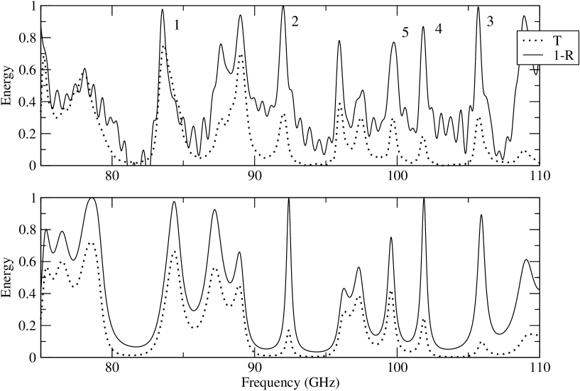
Figure 2: Measured (top) and calculated (bottom) transmission and reflection response for a randomly layered sequence of 100 quartz and Teflon disks. Plotted are the transmission coefficients ($T$, dotted curves) and one minus the reflection coefficient ($1-R$, solid curves).

In Fig. 2, we illustrate the transmission and reflection spectra for the W-band as investigated experimentally and theoretically for a representative sample. Plotted are the transmission coefficient ($T$) and one minus the reflection coefficient (R).

The actual data collection requires careful calibration of the system, in the instrument response and in all phase shifts in the cables and waveguide. First, one sweeps over the band of frequencies with no sample present; this gives a calibration E-field $E_{0}^{\mathrm{t}}$ measured for transmission. Second, one sweeps with a “perfect” reflector, i.e., a polished metal plate, at the focal plane; this gives a calibration E-field $E_{0}^{\mathrm{r}}$. Finally, with a sample in place, the sweep returns the amplitude and phase due to the presence of the sample relative to a flat instrument response. So, in Fig. 2, $R=|E^{r}/E_{0}^{r}|^{2}$ and $T=|E^{t}/E_{0}^{t}|^{2}$ are the reflection and transmission coefficients, respectively.

The theoretical curve in Fig. 2 is obtained by solving Maxwell’s equations numerically using the standard propagator matrix approach li:046607 . This allows us to compute the amplitude and phase of the reflected and transmitted fields as well as the fields everywhere inside the sample. As can be seen from Fig. 2, most frequencies lie in disorder-induced band-gaps, where the reflection coefficient is near unity. Between band-gaps there are narrow resonances accompanied by greatly enhanced transmission. Off-resonance transmission losses, e.g., around 80 and 94 GHz in Figure 2, are about 1%.

We observe in Fig. 2 differences in both amplitude and frequency between the measured and calculated spectra. In order to understand this effect, we studied periodic systems (data not shown), and found that the fit was better. We also studied many different random samples and did not find any systematic amplitude and frequency shifts. We conclude that these shifts are likely a random effect of the tiny, unmeasurable air gaps between wafers as well as of small random variations in the thicknesses of the wafers.

From the data shown in Fig. 2, the localization length $l_{\mathrm{loc}}$ can be estimated. Indeed, it is well known that the Lyapunov exponent, $\gamma\equiv l_{\mathrm{loc}}^{-1}=-(\ln T)/L$ is a self-averaging quantity lifshits ; sheng ; akkermans ; gantmakher . That is, its fluctuations are small and its variance tends to zero, so that

$$\gamma\rightarrow\langle\gamma\rangle\geq-(1/l_{\mathrm{loc}}+1/l_{\mathrm{abs}})\,,$$ (1)

where $L$ is the sample length and $l_{\mathrm{abs}}$ is the spatial absorption rate PhysRevB.50.6017 . Thus, at large $L$ the Lyapunov exponent $\gamma$ is close to $-(1/l_{\mathrm{loc}}+1/l_{\mathrm{abs}})$ with high probability, i.e., in almost all samples, or at almost all frequencies in one sample. We call such off-resonance samples and frequencies typical.

In Fig. 2, we find that $\gamma L$ at typical frequencies is approximately $0.01$. The measured loss tangents of quartz and Teflon correspond to absorption lengths of approximately 35 cm for quartz and 100 cm for Teflon. The reciprocal absorption length is $2\pi n\tan\delta/\lambda$, where $\tan\delta=\epsilon^{\prime\prime}/\epsilon^{\prime}$, $n$ is the index of the homogeneous material and $\lambda$ is the free-space wavelength of the probing beam. The absorption lengths of both quartz and Teflon are much larger than the sample itself. Thus, we find for our 42 mm sample the localization length $l_{\mathrm{loc}}=\gamma^{-1}\simeq 10$ mm. Since $l_{\mathrm{abs}}>>L$, its influence on typical transmission frequencies is negligible,

$$T_{\mathrm{typ}}\approx\exp(-L/l_{\mathrm{loc}}).$$ (2)

We reserve discussion of the atypical, or resonant case to Secs. IV and V.

IV Theoretical Description

As can be seen from Fig. 2, the sum of the reflection and transmission coefficients drops noticeably at the resonances. This means that absorption plays a significant role; in the presence of absorption, standard analytical treatments sheng ; akkermans ; gantmakher fall short. Therefore, we take advantage of an effective cavity model recently introduced by Bliokh et al. bliokh97 ; bliokh2004 as follows. In the random medium of our sample, the transmission coefficient at typical frequencies determines the localization length via Eq. (2) and so can be measured. However, along with the typical frequencies there are resonant frequencies. These are relatively rare, or low probability frequencies at which resonances occur, and the effect of absorption is dramatic. In these resonances, photons become partially trapped by multiple scattering. In effect, the random multiple scattering gives rise to an effective cavity within the sample. The long dwell time of these photons is responsible for the enhanced attenuation. In other words, the attenuation increases significantly at a resonance because the energy absorbed at each point is proportional to the intensity of the field, which is exponentially large throughout the resonant cavity. Therefore, both the reflection and transmission coefficients decrease sharply even when the absorption length $l_{\mathrm{abs}}$ is much larger than the total length $L$ of the sample.

One can treat any particular localized state as an effective cavity mode. Using the measurable reflection and transmission coefficients on and off resonance together with the measurable resonance width, one can make a fit to determine the location and width of the effective cavity, as well as an effective absorption length.

Consider a random sample as a 1D resonator built of a cavity of length $l_{\mathrm{cav}}$ bounded by two barriers of lengths $l_{1}$ and $l_{2}$, whose transmission coefficients are

$$T_{1,2}=\exp(-l_{1,2}/l_{\mathrm{loc}})\,,$$ (3)

with $l_{\mathrm{loc}}$ the localization length. The parameters of the effective cavity will be different for each resonance inside the same sample. We take as our starting point the resonant transmission and reflection coefficients and resonant width, which can be shown to be

$$R_{\mathrm{res}} = 1-{\frac{4}{\left(\sqrt{u/v}+\sqrt{v/u}\right)^{2}}}\,,$$ (4)

$$T_{\mathrm{res}} = {\frac{4}{(u+v)^{2}}}\,,$$ (5)

$$\delta\omega = \frac{c}{2\bar{\varepsilon}\,l_{\mathrm{cav}}}\sqrt{T_{1}T_{2}}(u+v)\,,$$ (6)

respectively, where $c$ is the speed of light in vacuum, $\bar{\varepsilon}$ is the average real part of the dielectric constant and $\delta\omega=2\pi\delta f$ is the resonance width. Here

$$u \equiv \sqrt{{\frac{T_{1}}{T_{2}}}},$$ (7)

$$v \equiv {\frac{G}{\sqrt{T_{1}T_{2}}}}+\sqrt{{\frac{T_{2}}{T_{1}}}}\,,$$ (8)

$$G \equiv 2\sqrt{{\bar{\varepsilon}}}\,l_{\mathrm{cav}}/l_{\mathrm{abs}}\,,$$ (9)

where $l_{\mathrm{abs}}$ is the effective absorption length such that the intensity $I$ decays as $\exp(-x/l_{\mathrm{abs}})$ in an ordinary random sample, and the total length of the sample is

$$L=l_{1}+l_{2}+l_{\mathrm{cav}}\,.$$ (10)

First, we determine the effective cavity length $l_{\mathrm{cav}}$. By definition,

$$T_{1}T_{2}=e^{-(L-l_{\mathrm{cav}})/l_{loc}}.$$ (11)

Substituting Eq. (11) and Eq. (5) into Eq. (6), one finds an implicit equation for the effective cavity length:

$$l_{\mathrm{cav}}=\frac{c}{\bar{\varepsilon}\,\delta\omega}\frac{1}{\sqrt{T_{\mathrm{res}}}}e^{-(L-l_{\mathrm{cav}})/(2l_{\mathrm{loc}})}\,.$$ (12)

This transcendental equation is analyzed in more detail in Sec. V.

Second, we determine the effective absorption length $l_{\mathrm{abs}}$. From Eqs. (7)-(9),

$$\frac{2\sqrt{\bar{\varepsilon}}\,l_{\mathrm{cav}}}{l_{\mathrm{abs}}}=\sqrt{T_{1}T_{2}}\left(v-u^{-1}\right)\,.$$ (13)

Then Eq. (11) implies

$$l_{\mathrm{abs}}=2\sqrt{\bar{\varepsilon}}\,l_{\mathrm{cav}}\left(v-u^{-1}\right)^{-1}e^{(L-l_{\mathrm{cav}})/(2l_{\mathrm{loc}})}.$$ (14)

Let us solve for $u,v$ as functions of $R_{\mathrm{res}},T_{\mathrm{res}}$ alone. Equations (4)-(5) yield

$$u^{2}+2uv+v^{2} = \frac{4uv}{1-R_{\mathrm{res}}},$$ (15)

$$u^{2}+2uv+v^{2} = \frac{4}{T_{\mathrm{res}}},$$ (16)

It follows that

$$v=\frac{1\pm\sqrt{R_{\mathrm{res}}}}{\sqrt{T_{\mathrm{res}}}},$$ (17)

$$u=\frac{1\pm\sqrt{R_{\mathrm{res}}}}{\sqrt{T_{\mathrm{res}}}},.$$ (18)

Equations (17) and (18) are valid only for $R_{\mathrm{res}}\neq 1$ and $T_{\mathrm{res}}\neq 0$. Substitution of Eqs. (17), (18), and (12) into Eq. (11) yields the absorption length:

$$l_{\mathrm{abs}}\equiv\frac{1}{\Gamma}=2\frac{c}{\delta\omega\sqrt{\bar{\varepsilon}}}\frac{1\pm\sqrt{R_{\mathrm{res}}}}{1-R_{\mathrm{res}}-T_{\mathrm{res}}}.$$ (19)

Third, we determine the length of the first barrier of the cavity, $l_{1}$. Substituting Eqs. (3) and (10) into Eq. (7), one obtains

$$u=e^{-l_{1}/l_{loc}}e^{(L-l_{\mathrm{cav}})/(2l_{\mathrm{loc}})}\,.$$ (20)

Eliminating $u$ with Eq. (18) and solving for $l_{1}$,

$$l_{1}={\frac{1}{2}}(L-l_{\mathrm{cav}})-l_{\mathrm{loc}}\ln\frac{1\pm\sqrt{R_{\mathrm{res}}}}{\sqrt{T_{\mathrm{res}}}}.$$ (21)

Finally, substituting Eq. (12) into Eq. (21), one finds the length of the first barrier:

$$l_{1}=-l_{\mathrm{loc}}\ln\left[{\frac{\bar{\varepsilon}\,\delta\omega\,l_{\mathrm{cav}}}{c}}\left(1\pm\sqrt{R_{\mathrm{res}}}\right)\right].$$ (22)

Equations (19), (12), and (22) present the absorption length and the effective cavity lengths in terms of measurable quantities, namely, the resonance transmission and reflection coefficients $T_{\mathrm{res}}$ and $R_{\mathrm{res}}$, the resonance width $\delta\omega=2\pi\delta f$, the average dielectric constant $\bar{\varepsilon}$, and the localization length determined via Eq. (2) from off-resonant transmission coefficients. In this treatment we have not taken advantage of the extra phase information that is obtained by our system. The phase provides an extra datum at each frequency which can be used to obtain additional cavity parameters.

Finally, it is also convenient to invert these equations for the ensuing discussion to obtain

$$T_{\mathrm{res}} = 4T_{1}T_{2}/(2l_{\mathrm{cav}}/l_{\mathrm{abs}}\sqrt{\bar{\varepsilon}}+T_{1}+T_{2})^{2},$$ (23)

$$R_{\mathrm{res}} = 1-\left(T_{2}+2l_{\mathrm{cav}}/l_{\mathrm{abs}}\sqrt{\bar{\varepsilon}}\right)T_{\mathrm{res}}/T_{2},$$ (24)

$$T_{1,2} \equiv \exp\left[-\left(l_{\mathrm{cav}}/2\pm\Delta d\right)/l_{\mathrm{loc}}\right],$$ (25)

where $\Delta d$ is the shift of the cavity’s center from that of the sample, replacing $l_{1}$.

Using data on the transmission and reflection coefficients and the peak widths for the sample shown in Figure 2 we have calculated internal parameters of our disordered system. These results are shown in Table I. Shown in columns 2,3 and 4 are $1-R$, $T$ and $\delta f$, respectively, measured for the resonances indicated in column 1. We use an extra vertical bar between columns 4 and 5 to emphasize the fact that the measured resonance values lie to the left of this double-bar and the retrieved system parameters lie to the right. The value of $\Gamma/\sqrt{\epsilon}$ (column 5) has been retrieved via equation 19. The loss tangent $\tan(\alpha)=\Gamma c/(2\pi f\sqrt{{\bar{\epsilon}}}$) is presented in column 6. The value of the loss tangent averaged over the five resonances equals $8.35\times 10^{-4}$. The weighted loss tangent for our disordered quartz/Teflon system is $5.2\times 10^{-4}$, so that the measured and retrieved values of the absorption agree to within the accuracy of the experiment. Thus from external measurements we have retrieved two internal parameters of the system, the localization length, which relates to disorder, and the absorption length.

frequency (GHz)	1-R	T	$\delta f$ (GHz)	$\Gamma/\sqrt{{\bar{\epsilon}}}\cdot 10^{2}$	$\tan\alpha\cdot 10^{4}$
$f_{1}=83.5$	.978	.75	.40	.83	4.77
$f_{2}=92.0$	.998	.33	.39	2.6	13.45
$f_{3}=105.7$	.993	.31	.34	2.25	10.14
$f_{4}=101.8$	.87	.18	.25	1.33	6.22
$f_{5}=99.8$	.77	.30	.45	1.5	7.16

Table 1: Measured and retrieved parameters associated with 5 resonances shown in Figure 2. The subscripts on the frequencies refer to the peaks indicated in the plot. The localization length is 1 cm, as obtained from the non-resonant transmission coefficient.

Finally, we note that numerical simulations were also performed with the standard propagator matrix method, as mentioned briefly in Sec. III, in order to obtain information about the electromagnetic field inside the sample. For these simulations we used the precise experimental ordering of quartz and Teflon wafers.

V Discussion

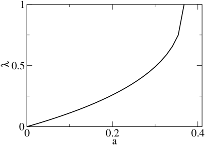
Figure 3: Shown is the solution to the transcendental Eq. (26), where $\lambda=l_{\mathrm{cav}}/2l_{\mathrm{loc}}$ and $a$ is given in Eq. (28).

Equation (12) requires further analysis, as it is transcendental. We can rescale it as

$$\lambda=a\exp(\lambda)\,,$$ (26)

where

$$\lambda \equiv l_{\mathrm{cav}}/2l_{\mathrm{loc}}\,,$$ (27)

$$a \equiv \frac{c}{2\,l_{\mathrm{loc}}\,\bar{\varepsilon}\,\delta\omega\,\sqrt{T_{\mathrm{res}}}}\exp(-L/2l_{\mathrm{loc}})\,.$$ (28)

Equation (26) has a real solution in terms of a ProductLog for $a\in(-\infty,1/e]$:

$$\lambda=-\mathrm{ProductLog}(-a)\,,$$ (29)

a special function which can be obtained numerically.

In the physical region of $a\in[0,1/e]$, $\lambda\rightarrow 1$ as $a\rightarrow 1/e$. Since the localization length must be smaller than the cavity size, it follows that $\lambda$ is confined to the relatively narrow range of $\frac{1}{2}e^{-\frac{1}{2}}\approx 0.3$ and $e^{-1}\approx 0.37$. Then the resonance width $\delta\omega$ must fall off exponentially as the system size is increased.

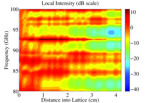
Figure 4: Localized E field within the sample. Shown is a plot of the calculated E-field intensity (in $dB$) within the scattering medium. By comparing the frequencies with those in Fig. 2 one can see the strong localization of the field at transmission resonances.

Figure 4 shows the calculated spatial distribution of the E-field inside the medium for the same sample as was used in Fig. 2, for both resonant and non-resonant frequencies. Figure 5 shows the spatial distribution of energy at three resonances.

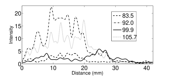
Figure 5: Localized modes at regions of enhanced absorption. E-field intensity as a function of space inside the sample at four resonant frequencies used in the analysis in Table I. Localization results in a varying degrees of field enhancement inside the random effective cavity. The stronger the field enhancement, the greater the path-length-induced absorption.

At resonance, the energy density within the localized mode, i.e., inside the effective cavity, can be orders of magnitude larger than that of the incident wave. This huge field enhancement has many potential applications. For example, at optical frequencies, this increased energy density has been exploited to produce a random laser lasers based on a layered (1D) medium. Off resonance, the dielectric multi-layer presents an almost perfect reflector; it is only the exponential tail of the field that penetrates the sample.

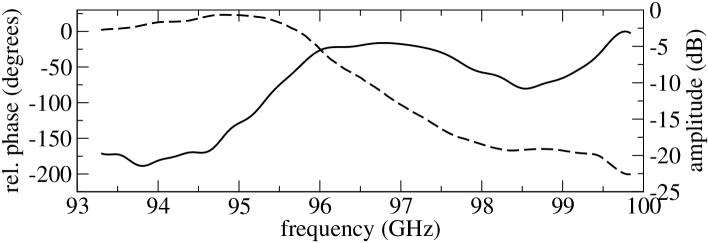
Figure 6: In order to interpret the fast and slow-light features of our measurement, we zoom in on a typical transmission resonance. For this purpose we could choose any of the resonances but here we zoom in around 97 GHz. We show the phase (dashed curve) and amplitude (solid curve) of the E-field transmitted through the same sample as in Figs. 2 and 4, as a function of frequency $f$ for the transmission resonance at 97 GHz. In band gaps the phase is nearly stationary while at resonance the inverse phase derivative, $(d\phi(f)/df)^{-1}$ decreases markedly.

Slow light is associated with strong dispersion and can be seen in situations involving resonant transmission, for example, with defect states in a band gap Bigelow07112003 or with ultracold atomic gases Hau . In the case of localization, slow light and enhanced absorption go hand in hand because they have the same physical origin – both of them are caused by multiple scattering, which increases dramatically the photon path and the resonance dwell time. Plotted in Fig. 6 is the measured frequency dependence of the phase, $\phi(f)$, of the signal transmitted through a random sample. At each resonance there is a pronounced decrease of the inverse phase derivative, $(d\phi(f)/df)^{-1}$. If there were a well defined group, i.e., a pulsed measurement, and if there were a well defined local wave number, then the inverse phase derivative would be proportional to the group velocity. For example, one could divide the transmitted phase by the thickness of the sample to get an average wave number. Such an analysis, however rough, gives group velocities on the order of 10% c. But our measurement doesn’t have sufficient bandwidth to synthesize pulses small compared to the size of the sample.

The corresponding time delay associated with a resonance can be estimated to be

$$\Delta t\propto\frac{1}{\Delta f}=\frac{l_{\mathrm{cav}}}{c\,T_{\mathrm{typ}}}\gg\frac{l_{\mathrm{cav}}}{c}.$$ (30)

Taking $l_{\mathrm{cav}}$ of the order of twice the localization length, $2\times 1$cm, and $T_{\mathrm{typ}}\simeq 0.01$, we obtain $\Delta t\propto l_{\mathrm{cav}}/c\times 1/T_{\mathrm{typ}}=2\>\mathrm{cm}\times 100/(3\times 10^{10}\mathrm{cm}/\mathrm{s})\approx 7$ ns. If we were speaking of well-defined pulses, such a delay would correspond to a group velocity an order of magnitude less than the speed of light. Although our measurements are fundamentally frequency-domain, the structure of the spectral peaks of the transmission coefficient can be related to the conventional notion of slow light in this sense.

VI Conclusions

We have developed an experimental system for studying disorder-induced wave phenomena in dielectrics at millimeter wave frequencies. In our system we see localization even in samples that are only four times the localization length. The deep resonances connected with localization allow one to observe enhanced absorption and disorder-induced delays that can be associated with group velocities much less than the speed of light in vacuum. Furthermore, off-resonance, the random dielectric stack becomes a near perfect reflector. This gives rise to a transmitted E-field phase that is nearly independent of frequency at the band-edge. We have interpreted the experimental data in terms of an effective cavity model, which enables us to retrieve the localization and absorption lengths from frequency dependent reflection and transmission coefficients.

This material is based upon work supported by the National Science Foundation under Grants EAR-0337379, EAR-041292 and PHY-0547845.

References

- (1) I. Lifshits, S. Gredeskul, and L. Pastur, Introduction to the theory of disordered systems (John Wiley and Sons, New York, 1988).
- (2) P. Sheng, Introduction to wave scattering, localization and mesoscopic phenomena (Springer, Berlin, 2006).
- (3) Éric Akkermans and G. Montambaux, Mesoscopic physics of electrons and photons (Cambridge University Press, Cambridge, 2007).
- (4) V. F. Gantmakher, Electrons and disorder in solids (Oxford Science Publications, Oxford, 2005).
- (5) D. Clement et al., Phys. Rev. Lett. 95, 170409 (2005).
- (6) C. Fort et al., Phys. Rev. Lett. 95, 170410 (2005).
- (7) T. Schulte et al., Phys. Rev. Lett. 95, 170411 (2005).
- (8) T. Paul, P. Schlagheck, P. Leboeuf, and N. Pavloff, Phys. Rev. Lett. 98, 210602 (2007).
- (9) V. Milner and A. Z. Genack, Physical Review Letters 94, 073901 (2005).
- (10) J. Bertolotti, S. Gottardo, and D. Wiersma, Physical Review Letters 92, 113903 (2005).
- (11) O. Shapira and B. Fischer, Journal of the Optical Society of America 22, 2542 (2005).
- (12) U. Kuhl, F. M. Izrailev, A. A. Krokhin, and H.-J. Stockmann, Applied Physics Letters 77, 633 (2000).
- (13) K. Y. Bliokh et al., Physical Review Letters 97, 243904 (2006).
- (14) J. F. Galisteo-Lopez et al., Physical Review B 73, 125103 (2006).
- (15) A. Hache and L. Poirier, Applied Physics Letters 80, 518 (2002).
- (16) C. Spielmann, R. Szipöcs, A. Stingl, and F. Krausz, Physical Review Letters 73, 002308 (1994).
- (17) E. Baldit et al., Physical Review Letters 95, 143601 (2005).
- (18) J. Heebner and R. Boyd, J of Modern Optics 49, 2629 (2002).
- (19) A. Yariv, Y. Xu, R. Lee, and A. Scherer, Optics Letters 24, 711 (1999).
- (20) P. Goldsmith, Quasioptical systems: Gaussian beams quasioptical propagation and applications (IEEE Press, New York, NY, 1998).
- (21) M. Mola, S. Hill, P. Goy, and M. Gross, Rev. Sci. Inst. 71, 186 (2000).
- (22) C. Dahl, P. Goy, and J. Kotthaus, in Millimeter and submillimeter wave spectroscopy in solids, edited by G. Grüner (Springer, Berlin, 1998), pp. 221–282.
- (23) Z.-Y. Li and L.-L. Lin, Physical Review E (Statistical, Nonlinear, and Soft Matter Physics) 67, 046607 (2003).
- (24) V. Freilikher, M. Pustilnik, and I. Yurkevich, Phys. Rev. B 50, 6017 (1994).
- (25) K. Y. Bliokh, Y. P. Bliokh, and V. Freilikher, J. Opt. Soc. Am. B 21, 113 (2004).
- (26) M. S. Bigelow, N. N. Lepeshkin, and R. W. Boyd, Science 301, 200 (2003).
- (27) L. V. Hau, S. E. Harris, Z. Dutton, and C. H. Behroozi, Nature 397, 594 (1999).