Transport and Percolation Theory in Weighted Networks

Abstract

We study the distribution $P(\sigma)$ of the equivalent conductance $\sigma$ for Erdős-Rényi (ER) and scale-free (SF) weighted resistor networks with $N$ nodes. Each link has conductance $g\equiv e^{-ax}$, where $x$ is a random number taken from a uniform distribution between 0 and 1 and the parameter $a$ represents the strength of the disorder. We provide an iterative fast algorithm to obtain $P(\sigma)$ and compare it with the traditional algorithm of solving Kirchhoff equations. We find, both analytically and numerically, that $P(\sigma)$ for ER networks exhibits two regimes. (i) A low conductance regime for $\sigma<e^{-ap_{c}}$ where $p_{c}=1/\langle k\rangle$ is the critical percolation threshold of the network and $\langle k\rangle$ is average degree of the network. In this regime $P(\sigma)$ is independent of $N$ and follows the power law $P(\sigma)\sim\sigma^{-\alpha}$, where $\alpha=1-\langle k\rangle/a$. (ii) A high conductance regime for $\sigma>e^{-ap_{c}}$ in which we find that $P(\sigma)$ has strong $N$ dependence and scales as $P(\sigma)\sim f(\sigma,ap_{c}/N^{1/3})$. For SF networks with degree distribution $P(k)\sim k^{-\lambda}$, $k_{min}\leq k\leq k_{max}$, we find numerically also two regimes, similar to those found for ER networks.

Recently much attention has been focused on complex networks which characterize many biological, social, and communication systems Albert02 ; Pastor ; Dorogovtsev ; Cohen . The networks are represented by nodes associated with individuals, organizations, or computers and by links representing their interactions. In many real networks, each link has an associated weight, the larger the weight, the harder it is to transverse the link. These networks are called “weighted” networks Brauns03 ; Barat .

Transport is one of the main functions of networks. While the transport on unweighted networks has been studied Lopez_transport , the effect of disorder on transport in networks is still an open question. Here we study the distribution $P(\sigma)$ of the equivalent electrical conductance $\sigma$ between two randomly selected nodes $A$ and $B$ on Erdős-Rényi (ER) E_R ; E_R2 and scale-free (SF) Albert02 weighted networks. We first provide an iterative fast algorithm to obtain $P(\sigma)$ for disordered resistor networks, and then we develop a theory to explain the behavior of $P(\sigma)$. The theory is based on the percolation theory Bunde for a weighted random network. We model a weighted network by assigning the conductance of a link connecting node $i$ and node $j$ as in Ref. Strelniker_2d_granular

$$g_{ij}\equiv\exp[-ax_{ij}],$$ (1)

where the parameter $a$ controls the broadness (“strength”) of the disorder, and $x_{ij}$ is a random number taken from a uniform distribution in the range [0,1]. We use this kind of disorder since a recent study of magnetorresistance in real granular materials systems Strelniker_2d_granular shows that the conductance is given by Eq. (1). Moreover, a recent study Chen_universal shows that many types of disorder distributions lead to the same universal behavior. The range of $a\gg 1$ is called the strong disorder (SD) limit Cieplak ; Porto . The special case of unweighted networks, i.e., $a=0$ or $g_{ij}=1$ for all links have been studied earlier Lopez_transport .

To construct ER networks of size $N$, we randomly connect nodes with $\langle k\rangle N/2$ links, where $\langle k\rangle$ is the average degree of the network. To construct SF networks, in which the degree distribution follows a power law, we employ the Molloy-Reed algorithm Molloy . The traditional algorithm to calculate the probability density function (pdf) $P(\sigma)$ is to compute $\sigma$ between two nodes $A$ and $B$ by solving the Kirchhoff equations with fixed potential $V_{A}=1$ and $V_{B}=0$ and compute $P(\sigma)d\sigma$, which gives the probability that two nodes in the network have conductance between $\sigma$ and $\sigma+d\sigma$. However, this method is time consuming and limited to relatively small networks. Here we also use an iteration algorithm proposed by Grimmett and Kesten net math to calculate $P(\sigma)$ and show that it gives the same results as the traditional Kirchhoff method.

Figure 1: Schematic Iteration model. In this example $R_{1}$ is infinite, so it is not taken into account in the sum in $R_{i}$ of Eq. (2).

In the limit $N\to\infty$ we ignore the loops between 2 randomly chosen nodes because the probability to have loops is very small. Hence the resistivity $R_{i}$ of a randomly selected branch $i$ connecting a node with infinitely distant nodes satisfies $R_{i}=r_{i}+1/(\sum_{j=1}^{k-1}R_{j}^{-1})$, where $r_{i}=e^{ax_{i}}$ is the random resistance of the link outgoing from this node and $k$ is a random number taken from the distribution $\tilde{p}_{k}=p_{k}\cdot k/\langle k\rangle$, which is the probability that a randomly selected link ends in a node of degree $k$, where $p_{k}$ is the original degree distribution. In Fig. 1, we show the schematic iteration method. The randomly selected nodes A and B are connected to the infinitely distant nodes C. When we calculate $R_{AC}$, the resistance between A and C, we perform the iterative steps as follows:

First we calculate the distribution of resistivities of the branches connecting node A with C. We start with $\cal{N}$ branches having resistivities $R_{i}^{(0)}=0\quad(i=1,2,...,\cal{N})$, where $\cal{N}$ is an arbitrary large number. Thus, initially the histogram of these resistivities $P_{0}(R)=\delta(R)$. At the iterative step $n+1$, we compute a new histogram $P_{n+1}(R)$ knowing the histogram $P_{n}(R)$. In order to do this we generate a new set of resistivities $R_{i}^{(n+1)}$ by connecting in parallel $k-1$ outgoing branches coming from a randomly selected node of degree $k$ obtained from the distribution $\tilde{p}_{k}=p_{k}\cdot k/\langle k\rangle$. Then we compute the resistivity of a branch going through this node via an incoming link with a random resistivity $r_{i}^{(n)}$ taken from the link resistivity distribution,

$$R_{i}^{(n+1)}=r_{i}^{(n)}+{1\over\sum_{j=1}^{k-1}1/R_{j}^{(n)}}.$$ (2)

In Eq. (2), if at least one of the terms $R_{i}^{(n)}=0$, we take $R_{i}^{(n+1)}=r_{i}^{(n)}$. Thus after the first iterative step $P_{1}(R)$ coincides with the distribution of link resistivities.

According to the theorem proved in net math , as $n\to\infty$, $P_{n}(R)$ converges to a distribution of the resistivities of a branch connecting a node to the infinitely distant nodes. The resistivity between a randomly selected node of degree $k$ and the infinitely distant nodes is defined by

$$\tilde{R}_{(i)}={1\over\sum_{j=1}^{k}1/R_{j}},$$ (3)

where $k$ is selected from the original degree distribution $p_{k}$ and $R_{j}$ is selected from $P_{n\to\infty}(R)$.

Finally, to compute the resistivity $R_{ij}$ between two randomly selected nodes $i$ and $j$ (for example $A$ and $B$ in Fig. 1), we compute $R_{ij}=\tilde{R}_{(i)}+\tilde{R}_{(j)}$, where $\tilde{R}_{(i)}$ and $\tilde{R}_{(j)}$ are randomly selected resistivities between a node and the infinitely distant nodes. If $\cal{N}$ is a sufficiently large number, we find the conductance distribution $P(\sigma)$ between any two randomly selected nodes.

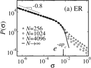
Figure 2: Plots of $P(\sigma)$ for several values of $N$. The symbols are for the Kirchhoff method and the solid line is for the iterative method with $N\to\infty$. (a) ER networks with fixed $\langle k\rangle=3$ and $a=15$. (b) SF networks with fixed $\lambda=3.5$, $k_{\rm min}=2$, $\langle k\rangle\approx 3.33$ and $a=20$. The dashed line slopes are from the prediction of Eq.(11) or (13).

In Figs. 2(a) and 2(b) we show the results of $P(\sigma)$ using the traditional method of solving Kirchhoff’s equations for different values of $N$ and the iterative method with $N\to\infty$ for both ER and SF networks. We see that the main part of the distribution (low conductances) does not depend on $N$, and only the high conductance tail depends on $N$.

The behavior of the two regimes, low conductance and high conductance, can be understood qualitatively as follows: For strong disorder $a\gg 1$ all the current between two nodes follows the optimal path between them. The problem of the optimal path in a random graph in the strong disorder limit can be mapped onto a percolation problem on a Cayley tree with a degree distribution identical to the random graph and with a fraction $p$ of its edges conducting santafe . However, the conductance on this path is determined by the bond with the lowest conductance $e^{-ax_{max}}$, where $x_{max}$ is the maximum random number along the path. In the majority of cases $x_{max}>p_{c}$, where $p_{c}$ is the critical percolation threshold of the network, and only when the two nodes both belong to the incipient infinite percolation cluster (IIPC) Bunde , $x_{max}<p_{c}$. Since the size of the IIPC scales as $N^{2/3}$, the probability of randomly selecting a node inside the IIPC is proportional to $N^{2/3}/N=N^{-1/3}$ E_R ; E_R2 ; Bunde . Then the probability of randomly selecting a pair inside the IIPC is proportional to $(N^{-1/3})^{2}=N^{-2/3}$. These nodes contribute to the high conductance range $\sigma>e^{-ap_{c}}$ of $P(\sigma)$. The low conductance regime is determined by the distribution of $x_{max}$, that follows the behavior of the order parameter $P_{\infty}(p)$ (for $p>p_{c}$) in the percolation problem which is independent of $N$ santafe . (This will be explained later in the theoretical approach for the low conductance regime.)

We call the low conductance regime a non-percolation regime and the high conductance regime a percolation regime. In contrast, the property of existing two regimes does not show up in the optimal path length Tomer-op ; Wu_flow and only the scaling regime with $N$ appears. This is since the path length for almost all pairs is dominated by the IIPC Wu_flow .

In Figs. 3(a) and 3(b) we plot for a given $N$ only the non-percolation part of $P(\sigma)$ as a function of $\sigma$ for fixed values of $\langle k\rangle/a$ and different $\langle k\rangle$ and $a$ values for ER networks. We see that it obeys a power law with the slope $\langle k\rangle/a-1$ for $\sigma<e^{-ap_{c}}$. Note that for ER networks $p_{c}=1/\langle k\rangle$ E_R ; E_R2 . In Fig. 3(c), we plot the conductance distribution for SF networks for fixed values of $\langle k\rangle/a$. We can see the non-percolation part seems to obey the same power law as ER networks.

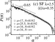
Figure 3: Plots of $P(\sigma)$ for fixed $\langle k\rangle/a$. The symbols are for the Kirchhoff method and the solid line is for the iterative method. For the same $\langle k\rangle/a$, the iterative method for different $a$ shows the same $P(\sigma)$ except that the lower cutoff is different. (a) ER network with $\langle k\rangle/a=0.2$. (b) ER network with $\langle k\rangle/a=1.5$. (c) SF network with $\langle k\rangle/a\approx 0.35$, $\lambda=2.5$. The dashed line slopes are from the prediction of Eq.(11) or (13).

Next we present an analytical approach for the form of $P(\sigma)$ for low conductance regime. The distribution of the maximal random number $x_{\rm max}$ along the optimal path can be expressed in terms of the order parameter $P_{\infty}(p)$ in the percolation problem on the Cayley tree, where $P_{\infty}(p)$ is the probability that a randomly chosen node on the Cayley tree belongs to the IIPC santafe . For a random graph with degree distribution $p_{k}$, the probability to arrive at a node with $k$ outgoing branches by following a randomly chosen link is $(k+1)p_{k}/\langle k\rangle$ branch theo . The probability that starting at a randomly chosen link on a Cayley tree one can reach the $\ell$th generation is

$$f_{\ell}(p)\equiv f_{\ell}=1-\sum_{k=1}^{\infty}\frac{p_{k}k\left(1-pf_{{\ell}-1}\right)^{k-1}}{\langle k\rangle},$$ (4)

where $f_{0}=1$. Slightly different from $f_{\ell}$ is the probability that starting at a randomly chosen node one can reach the $n$th generation,

$$\tilde{f}_{n}=1-\sum_{k=0}^{\infty}p_{k}(1-pf_{n-1})^{k}.$$ (5)

In the asymptotic limit $f_{\ell}$ converges to $P_{\infty}$ for a given value of $p$,

$$f_{\ell}\to P_{\infty}(p)=1-\sum_{k=1}^{\infty}\frac{p_{k}k\left(1-pP_{\infty}\right)^{k-1}}{\langle k\rangle}.$$ (6)

In this limit we have a pair of nodes on a random graph separated by a very long path of length $n$. The probability that two nodes will be connected (conducting) at given $p$, can be approximated by the probability that both of them belong to the IIPC net math :

$$\Pi(p)=\left[{\tilde{P}_{\infty}(p)\over\tilde{P}_{\infty}(1)}\right]^{2},$$ (7)

where $\tilde{P}_{\infty}(p)\equiv\lim_{n\to\infty}\tilde{f}_{n}=1-\sum_{k=0}^{\infty}p_{k}(1-pP_{\infty})^{k}$. Note that the negative derivative of $\Pi(p)$ with respect to $p$ is the distribution of $x_{max}$ and thus gives $P(\sigma)$ in the SD limit. In our case $\sigma=e^{-ap}$, so replacing $p$ by $p=-\ln\sigma/a$ in Eq. (7) and differentiating with respect to $\sigma$, we obtain the distribution of conductance in the SD limit when the source and sink are far apart ($n\to\infty$),

$$P(\sigma)=-{d\over d\sigma}\Pi(\sigma)=\frac{2\tilde{P}_{\infty}(p)}{\sigma a[\tilde{P}_{\infty}(1)]^{2}}\cdot\frac{\partial\tilde{P}_{\infty}(p)}{\partial p}~{}\mid_{p=-\ln\sigma/a}.$$ (8)

For ER networks the degree distribution is a Poisson distribution with $p_{k}=\langle k\rangle^{k}e^{-\langle k\rangle}/k!$ E_R ; E_R2 and thus $P_{\infty}(p)$ satisfies

$$P_{\infty}(p)=1-e^{-\langle k\rangle pP_{\infty}(p)},$$ (9)

which has a positive root $P_{\infty}$ for $p>p_{c}=1/\langle k\rangle$. And $\tilde{P}_{\infty}(p)=P_{\infty}(p)$, thus

$$P(\sigma)=\frac{2P_{\infty}(p)}{\sigma a[P_{\infty}(1)]^{2}}\cdot\frac{\partial P_{\infty}(p)}{\partial p}~{}\mid_{p=-\ln\sigma/a},$$ (10)

where $P_{\infty}(p)$ and $P_{\infty}(1)$ are the solutions of Eq. (9).

We test the analytical result Eq. (10) by comparing the numerical solution of Eqs. (9) and (10) with the simulations on actual random graphs by solving Kirchhoff equations (Figs. 2 and 3). The agreement between the simulations and the theoretical prediction is perfect in the SD limit, i.e. when $\langle k\rangle/a$ is small.

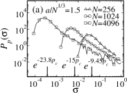
Figure 4: Kirchhoff method results of the percolation part of ER networks with the same value of $p_{c}=1/\langle k\rangle=0.33$. (a) Normalized $P_{p}(\sigma)$ for fixed $a/N^{1/3}=1.5$. (b) Scaled plot of $\langle\sigma\rangle P(\sigma)$ as function of $\sigma/\langle\sigma\rangle$ for three values of $a/N^{1/3}$. For each value of $a/N^{1/3}$, the thick line is for $N=256$ and the thin line is for $N=1024$.

Next we simplify $P(\sigma)$ from Eq. (10). Assuming that $P_{\infty}(1)\approx 1$ which is true for large $\langle k\rangle$ and approximating a slow varying function $P_{\infty}(p)$ by $P_{\infty}(1)$ we obtain

$$P(\sigma)\approx 2\frac{\langle k\rangle}{a}\sigma^{\langle k\rangle/a-1},$$ (11)

for the range $e^{-a}\leq\sigma\ll e^{-ap_{c}}$ with $p_{c}=1/\langle k\rangle$. In Figs. 2 and 3 we also show the results predicted by Eq. (11). For an infinite network, for $p\leq p_{c}=1/\langle k\rangle$, $P_{\infty}(p)=0$, and hence, the distribution of conductances must have a cutoff at $\sigma=e^{-ap_{c}}$. Indeed, in Fig. 2(a) and Figs. 3(a) and 3(b) we see that the upper cutoff of the iterative curves is close to $e^{-ap_{c}}$.

As discussed above, the range of high conductivities corresponds to the case where both the source and the sink are on the IIPC. Previously we found this percolation part to scale as $N^{-2/3}$. Using Fig. 2(a), we compute the integral for each $P(\sigma)$ from $e^{-ap_{c}}$ to $\infty$, and find that indeed $\int_{e^{-ap_{c}}}^{\infty}P(\sigma)\mathrm{d}\sigma\sim N^{-2/3}$, in good agreement with the theoretical approach. To show how the percolation part of $P(\sigma)$ is related to the parameters $N$, $a$ and $p_{c}$, we analyze the conductance between pairs on the IIPC, i.e., each link on the optimal path from source to sink has $x$ less than $p_{c}$. We compute $P_{p}(\sigma)$ of these pairs on the IIPC. When we simulate this process, we have only $N^{-2/3}$ probability to find this part from the original normalized distribution $P(\sigma)$. Thus, we normalize $P_{p}(\sigma)$ by dividing by $N^{-2/3}$. Figures 4(a) and 4(b) show the normalized $P_{p}(\sigma)$ of pairs on the IIPC. In this range, we see that $P_{p}(\sigma)$ is dominated by high conductivities and we find $\langle\sigma\rangle\approx e^{-ap_{c}}$ and

$$\langle\sigma\rangle P_{p}(\sigma)=f\left({\sigma\over\langle\sigma\rangle},{ap_{c}\over N^{1/3}}\right),$$ (12)

that is, for fixed $ap_{c}/N^{1/3}$, $\langle\sigma\rangle P_{p}(\sigma)$ scales with $\sigma/\langle\sigma\rangle$ as seen in Fig. 4(b). The scaled distributions have the same shape for the same $ap_{c}/N^{1/3}$ which specifies the strength of disorder similarly to the behavior of the optimal path lengths Chen_universal ; Tomer-op ; Wu_flow ; sameet_opt . The explanation of this fact for the distribution of conductances is analogous to the arguments presented in Refs. santafe and Tomer-op for the distribution of the optimal path. Thus the position of the maximum of the scaled curves in Fig. 4(b), and the whole shape of the distributions, depend on $ap_{c}/N^{1/3}$.

We also find that the extreme high conductivities correspond to the case where source and sinks are separated by only one link. In this case, $P(\sigma)=\frac{\langle k\rangle}{aN\sigma}\sim\sigma^{-1}$, ($\sigma<1$).

In summary, we find that $P(\sigma)$ exhibits two regimes. For $\sigma<e^{-ap_{c}}$, we show both analytically and numerically that for ER networks $P(\sigma)$ follows a power law,

$$P(\sigma)\sim\sigma^{-\alpha}\qquad[\alpha=1-\langle k\rangle/a].$$ (13)

We also find that for SF networks, Eq. (13) seems to be a good approximation, consistent with numerical simulations. The distributions of optimal path length and the path length of the electrical currents in complex weighted networks Tomer-op ; Wu_flow have been found to depend on $N$ for all length scales and all types of networks studied. In contrast, here we find that the low conductance tail of $P(\sigma)$ does not depend on $N$ for both ER and SF networks. However, the high conductance regime ($\sigma>e^{-ap_{c}}$) of $P(\sigma)$ does depend on $N$, in a similar way to the optimal path length and current path length distributions Tomer-op ; Wu_flow .

We thank ONR, Dysonet, FONCyt (PICT-O 2004/370), FONCyt (PICT-O 2004/370), Israel Science Foundation and Conycit for support, and Zhenhua Wu for helpful discussions.

References

- (1) R. Albert and A.-L. Barabási, Rev. Mod. Phys. 74, 47 (2002).
- (2) S. N. Dorogovtsev and J. F. F. Mendes, Evolution of Networks: From Biological Nets to the Internet and WWW (Oxford University Press, Oxford, 2003).
- (3) R. Pastor-Satorras and A. Vespignani, Structure and Evolution of the Internet: A Statistical Physics Approach (Cambridge University Press, Cambridge, 2004).
- (4) R. Cohen and S. Havlin, Complex networks: Stability, Structure and Function (Cambridge University Press, Cambridge, In press).
- (5) L. A. Braunstein et al., Phys. Rev. Lett. 91, 168701 (2003).
- (6) A. Barrat, M. Barthélemy, R. Pastor-Satorras and A. Vespignani, PNAS 101, 3747(2004).
- (7) E. López et al., Phys. Rev. Lett. 94, 248701 (2005).
- (8) P. Erdős and A. Rényi, Publ. Math. (Debrecen) 6, 290 (1959).
- (9) P. Erdős and A. Rényi, Publications of the Mathematical Inst. of the Hungarian Acad. of Sciences 5, 17 (1960).
- (10) A. Bunde and S. Havlin, Fractals and Disordered Systems (Springer-Verlag, Heidelberg, 1995).
- (11) Y. M. Strelniker et al., Phys. Rev. E 69, 065105(R) (2004).
- (12) Y. Chen et al., Phys. Rev. Lett. 96, 068702 (2006).
- (13) M. Cieplak et al., Phys. Rev. Lett. 72, 2320 (1994); 76, 3754 (1996).
- (14) M. Porto et al., Phys. Rev. E 60, R2448 (1999).
- (15) M. Molloy and B. Reed, Random Structures and Algorithms 6, 161 (1995); Combin. Probab. Comput. 7, 295 (1998).
- (16) G. Grimmett and H. Kesten, Random electrical networks on complete graphs II: Proofs, 1983 (http://arxiv.org/abs/math.PR/0107068).
- (17) L. A. Braunstein et al., in Lecture Notes in Physics: Proceedings of the 23rd CNLS Conference, “Complex Networks,” Santa Fe 2003, edited by E. Ben-Naim, H. Frauenfelder, and Z. Toroczkai (Springer, Berlin, 2004).
- (18) T. Kalisky et al., Phys. Rev. E 72, 025102(R) (2005).
- (19) Z. Wu et al., Phys. Rev. E 71, 045101(R) (2005).
- (20) T. E. Harris, The Theory of Branching Processes (Dover Publication Inc., New York, 1989).
- (21) S. Sreenivasan et al., Phys. Rev. E 70, 046133 (2004).