Analytical Solution to Transport in Brownian Ratchets via Gambler’s Ruin Model

Abstract

We present an analogy between the classic Gambler’s Ruin problem and the thermally-activated dynamics in periodic Brownian ratchets. By considering each periodic unit of the ratchet as a site chain, we calculated the transition probabilities and mean first passage time for transitions between energy minima of adjacent units. We consider the specific case of Brownian ratchets driven by Markov dichotomous noise. The explicit solution for the current is derived for any arbitrary temperature, and is verified numerically by Langevin simulations. The conditions for vanishing current and current reversal in the ratchet are obtained and discussed.

In the Gambler’s Ruin problem, a player plays a series of games against an adversary, winning (or losing) one dollar for every success (or failure), until one of them is “ruined”. Given the probability of winning each game, the Gambler’s Ruin problem considers the probability of ultimate ruin of one of the players, as well as the number of games required Feller (1968). In this paper, we show an intimate relationship between this classic random walk problem and the thermally activated dynamics in arbitrary potentials. The linkage between these two disparate topics is made possible by recent advances in the time quantification (TQ) of Monte Carlo (MC) Cheng et al. (2006); Kikuchi et al. (1991). In particular, the evolutionary techniques for the Gambler’s Ruin problem can be utilized to analyze the transition probabilities and the mean first passage time (MFPT) of the complex stochastic transport in Brownian ratchets.

An oscillating driving force applied on Brownian particles in asymmetric periodic potentials (ratchets) can cause directed transport, i.e. imbalanced current Reimann (2002); Astumian and Bier (1994); Doering et al. (1994). The keen scientific interest in the transport property of Brownian ratchets is attributed to their role in biological systems, e.g. the astonishing energy-motion conversion of ATP hydrolysis Svoboda et al. (1993). One of the key questions in the study of Brownian ratchets is obtaining the expression for current. In general, the stochastic transport in the ratchets is modeled by Langevin equations of the form:

$$\gamma\dot{x}=-U^{\prime}(x,z(t))+\xi(t),$$ (1)

where $\xi(t)$ is a mean zero Gaussian white noise term, i.e. $\left<\xi(t)\xi(s)\right>=2\gamma k_{B}T\cdot\delta(t-s)$, and $z(t)$ is a Markov dichotomous process with correlation time $\tau_{c}$. $\xi(t)$ represents the effects of thermal fluctuation, while $z(t)$ models stochastic processes such as impurities or defects jumping between metastable states Kula et al. (1998). The current is calculated by solving the corresponding Fokker-Planck equation (FPE) under periodic boundary conditions. However the explicit current expression can only be obtained for a few simple cases Kula et al. (1998); Van den Broeck et al. (2004); Reimann and Elston (1996), due to the complexity of dichotomous processes induced dynamics. For non-trivial cases, the ratchet current can be calculated by simulating the Langevin equation Lindner et al. (1999) or from numerical solutions of the FPE Bier and Astumian (1996).

Numerical calculations are computationally intensive and do not yield as much physical insights as analytical solutions. Our objective is thus to derive the analytical expression of the current for an arbitrary ratchet potential. This is performed by first discretizing each periodic unit of the ratchet into a finite site chain with absorbing boundaries and analyzing the random walk within this chain. This is essentially the classic Gambler’s Ruin problem, with some modifications to account for the dichotomous process. To complete the analogy, the corresponding time (in seconds) of one Monte Carlo step (MCS) has to be justified. Drawing from recent advances in quantifying the MCS Cheng et al. (2006); Kikuchi et al. (1991), e.g. by linking the MC scheme to the Langevin dynamics via the FPE Cheng et al. (2006), we formulate a time-quantification technique based on the Central Limit Theorem (CLT). With this, we established the theoretical basis for the analytical expression of the ratchet current obtained through the MC approach.

To explain our formalism, we shall first introduce time quantification of the MCS based on the CLT. Next, we model the transport in a Brownian ratchets with MC formalism and derive the transition probability and the MFPT in each periodic unit, and hence the ratchet current. The current expression is obtained for the simple thermal equilibrium case, and the more complex case of dichotomous noise. Finally, by applying the aforementioned TQ factor the current expression is verified by means of numerical Langevin simulation.

Time quantification of the MCS is most easily introduced by considering an overdamped Brownian particle in a steady potential $U(x,z(t))=V(x)$. The random walk on $x$ takes a fixed length trial move: $\Delta x=-R,R$ ($R\ll 1$) with equal trial probability in both directions but subject to the heat-bath acceptance rate of $1/(1+\exp(\beta\Delta V))$. Here $\Delta V$ is the energy difference in the proposed transition and $\beta\equiv 1/k_{B}T$. Expanding the heat-bath acceptance rate, we obtain the mean $\mu$ and variance $\sigma$ of $\Delta x$ in one MCS: $\mu=\frac{1}{4}\beta f(x_{0})R^{2}$ and $\sigma^{2}=\frac{1}{2}R^{2}+O(R^{4})$ , where $f(x)=-V^{\prime}(x)$ is the external force. Since $R\ll 1$, the change of $f(x)$ within a few MCS is negligible. According to the CLT, after a large number $n$ MCS the spread of displacement from $x_{0}$ approximates the normal distribution:

$$P(\Delta x_{\mathrm{MC}})=N(n\mu,n\sigma^{2})=f(x_{0})\cdot n\frac{1}{4}\beta R^{2}+\eta\sqrt{2n\frac{1}{4}R^{2}},$$ (2)

where $\eta\!\sim\!N(0,1)$ follows the standard Gaussian distribution. We note that the integration form (Ito’s interpretation) of the overdamped Langevin equation of Eq. (1) also results in a normal distribution of the displacement $\Delta x$ after a time interval $\Delta t$:

$$P(\Delta x_{\mathrm{LD}}) = \frac{1}{\gamma}f(x_{0})\Delta t+\eta\sqrt{2(k_{B}T/\gamma)\Delta t}.$$ (3)

Comparing Eq. (2) and Eq. (3), we obtain a term-by-term equivalence between $\Delta x_{\mathrm{MC}}$ and $\Delta x_{\mathrm{LD}}$ if

$$1\;\mathrm{MCS}=\Delta t/n=\gamma\beta R^{2}/4.$$ (4)

Since the dichotomous process $z(t)$ simply produces transitions between the two potential profiles, the equivalence established in Eq. (4) is still valid in the presence of $z(t)$, subject to the condition that $\Delta t\ll\tau_{c}$. This equivalence justifies the use of MC methods to analyze the ratchet current instead of the Langevin equation.

Figure 1: Schematic diagram of a $L$-periodic ratchet potential.

We consider an $L$-periodic ratchet which can be divided into “supersites” of length $L$, e.g. sites $i-1$, $i$ and $i+1$, as shown in Fig. (1). The forward and backward transition probability between the supersites, defined as $g\equiv p(x\to x+L)$ and $h\equiv p(x\to x-L)$, respectively, should be constant for all $x$ corresponding to an energy minimum, due to the periodic property. The difference between the transition probabilities of $g$ and $h$ results in a non-zero current. We hence have the steady current:

$$\left<\dot{x}\right>:=\lim_{t\to\infty}\frac{x(t)-x(0)}{t}=\frac{(g-h)L}{\tau_{\mathrm{\scriptscriptstyle MFPT}}},$$ (5)

where $\tau_{\mathrm{\scriptscriptstyle MFPT}}$ is the MFPT for the particle starting at position $x_{0}$ to hit either position $x_{0}+L$ or $x_{0}-L$. $\tau_{\mathrm{\scriptscriptstyle MFPT}}$ is a critical factor in influencing the transport in the ratchets and has been studied for several limited cases Reimann and Elston (1996); Iwaniszewski (2003).

We start our analysis with a simple illustrative case – a thermal equilibrium Brownian ratchets without a driven noise. We first discretize the ratchets of length $2L$ into $2N+1$ micro-sites, i.e. $\{S_{0},\ldots,S_{2N}\}$ as illustrated in Fig. (1). A particle starts at site $S_{m}$, and moves to adjacent micro-sites randomly, e.g. with steady probability $\mu_{m}$ to site $S_{m-1}$ and with probability $w_{m}$ to site $S_{m+1}$. We define $g(m)$ as the probability that the particle from site $S_{m}$ reach the end site $S_{2N}$ before it reaches the site $S_{0}$. We further define $\tau(m)$ as the MFPT (in MCS) for the particle to reach either end site $S_{0}$ or $S_{2N}$. Hence, we obtain the difference relations for $g(m)$ and $\tau(m)$:

$$g(m) = \mu_{m}\cdot g(m-1)+w_{m}\cdot g(m+1)+(1-\mu_{m}-w_{m})\cdot g(m)$$ (6)

$$\tau(m) = \mu_{m}\cdot\tau(m-1)+w_{m}\cdot\tau(m+1)+(1-\mu_{m}-w_{m})\cdot\tau(m)+1,$$ (7)

which are analagous to those of the Gambler’s Ruin problem. The initial conditions $g(0)=0$, $g(2N)=1$ and $\tau(0)=\tau(2N)=0$ apply.

The solution to Eq. (6) can be obtained by the recurrence relation: $g(m+1)-g(m)=(\mu_{m}/w_{m})(g(m)-g(m-1))$. Starting from the middle minima i.e. $m=N$, we can obtain the forward transition probability $g$ between the adjacent supersites:

$$g=g(N)=\frac{\sum^{N-1}_{i=0}k(i)}{\sum^{2N-1}_{i=0}k(i)}=\frac{1}{1+k(N)},$$ (8)

where $k(0)\equiv 1$, $k(m)\equiv\prod^{m}_{i=1}\mu_{i}/w_{i}$ for $m\geq 1$. In the last step we have used the periodic condition: $\mu_{j}=\mu_{N+j}$ and $w_{j}=w_{N+j}$, which leads to $k(N+i)=k(N)\cdot k(i)$. The backward transition probability can be obtained immediately from $h=(1-g)$. Similarly for Eq. (7), after some simplification we obtain, for $m=N$:

$$\tau_{\mathrm{\scriptscriptstyle MFPT}}=\tau(N)=g\cdot\sum_{i=1}^{N}\left((w_{i}k(i))^{-1}\sum_{j=i}^{N+i-1}k(j)\right).$$ (9)

Substituting the heat-bath rate definition $\frac{1}{1+\exp(\beta\Delta V)}$ for $w_{i}$ and $\mu_{i}$ into $k(i)$, we obtain: $k(i)=(w_{0}/w_{i})e^{\beta V_{i}}=2w_{0}(e^{\beta V_{i}}+e^{\beta V_{i+1}})$, where $V_{i}$ is the potential at the $i$th site and $V_{0}\equiv 0$. Particularly, $k(N)=\exp(\beta V_{N})$ since $w_{0}=w_{N}$. Thus, by considering Eqs. (4) and (5), the current expression for ratchets in thermal equilibrium converges to the well-discussed continuous form Risken (1967) as $N\to\infty$:

$$\left<\dot{x}\right>=\frac{(g-h)L}{\tau_{\mathrm{\scriptscriptstyle MFPT}}}=\frac{L\cdot(1-e^{\beta V(L)})}{\gamma\beta\int_{0}^{L}dx\;e^{-\beta V(x)}\int_{x}^{x+L}dy\;e^{\beta V(y)}}.$$ (10)

We shall also point out that for $N=2$, our above discussion reduces to the three-state discrete-time minimal Brownian ratchet model Lee et al. (2003). In particular, if we replace the transition rates with $\mu^{\prime}_{i}=\tilde{\gamma}\mu_{i}+\gamma/2$ and $w^{\prime}_{i}=\tilde{\gamma}w_{i}+\gamma/2$ following the definitions in Ref. Lee et al. (2003), we achieve the same current expression via Eq. (5) directly.

We now extend our discussion to the non-equilibrium case, i.e. with an additional dichotomous noise $z(t)$ applied to the ratchets potential. We consider a mean-zero $z(t)$, which takes two discrete values $\{1,-\theta\}(\theta>0)$ with correlation $\left<z(t)z(s)\right>=(Q/\tau_{c})\exp(-|t-s|/\tau_{c})$, where $Q=\theta\tau_{c}$. For clarity, we denote “$+$” and “$-$” as representing the two states $z=1$ and $z=-\theta$ respectively. Similar to our previous analysis, we define $g(m;\sigma;\sigma^{\prime})$ as the probability for a particle at initial site $S_{m}$ with $z(t_{0})=\sigma$ to reach the end site $S_{2N}$ after some time $t$ with $z(t)=\sigma^{\prime}$ before it reaches site $S_{0}$. We also define $\tau(m;\sigma)$ as the MFPT for the particle starting at $S_{m}$ under $z(t_{0})=\sigma$ to reach any end sites.

We first calculate the $g(m;\sigma;\sigma^{\prime})$, by considering the following four difference equations:

$$g(m;\sigma;\sigma^{\prime})=\sum_{\tilde{\sigma}}v(\tilde{\sigma}|\sigma)\cdot\left[w_{m}^{\tilde{\sigma}}g(m+1;\tilde{\sigma};\sigma^{\prime})+\mu_{m}^{\tilde{\sigma}}g(m-1;\tilde{\sigma};\sigma^{\prime})+(1-w_{m}^{\tilde{\sigma}}-\mu_{m}^{\tilde{\sigma}})g(m;\tilde{\sigma};\sigma^{\prime})\right],$$ (11)

where $v(\tilde{\sigma}|\sigma)$ is the transition probability for dichotomous state from $\sigma$ to $\tilde{\sigma}$ in one MCS Barik et al. (2006). $w_{m}^{\sigma}$ and $\mu_{m}^{\sigma}$ denote the spatial transition rates at dichotomous state $z(t)=\sigma$. Equation (11) can be rewritten into a $2\times 2$ matrix difference equation. After some algebra, we obtain:

$$X_{m+1}=W_{m}^{-1}\left(\lambda\cdot C+W_{m}+U_{m}\right)\cdot X_{m}-W_{m}^{-1}U_{m}\cdot X_{m-1},$$ (12)

where $\lambda\equiv\frac{v(-|+)}{1-v(-|+)-v(+|-)}\ll 1$, $W_{m}=\mathrm{Diag}\{w_{m}^{+},w_{m}^{-}\}$, $U_{m}=\mathrm{Diag}\{\mu_{m}^{+},\mu_{m}^{-}\}$, and

$$C=\left({\begin{array}[]{cc}{1}&{-1}\\ {-\theta}&{\theta}\\ \end{array}}\right);\quad X_{m}=\left({\begin{array}[]{*{20}c}{g(m;+;+)}&{g(m;+;-)}\\ {g(m;-;+)}&{g(m;-;-)}\\ \end{array}}\right).$$

The initial conditions are $X_{0}=\mathbf{0}$; $X_{2N}=\mathrm{Diag}\{1,1\}\equiv I$. The additional correlation term $(\lambda\cdot C)$ in Eq. (12) prevents a general solution for $X_{m}$. Nevertheless $X_{m}$ can be reduced into a linear combination of $X_{1}$ and $X_{0}$ by recurring Eq. (12). Since $X_{0}=\mathbf{0}$, we can thus define a $2\times 2$ matrix $Q_{m}$ such that

$$X_{m}=Q_{m}\cdot X_{1}\hskip 7.22743pt(m\geq 1).$$ (13)

$Q_{m}$ can be expressed as a polynomial function of $\lambda$:

$$Q_{m}(\lambda)=\sum_{l=0}^{m-1}D_{l}^{m}\cdot\lambda^{l},$$ (14)

where $D_{l}^{m}$ are $2\times 2$ matrices which are given by:

$$D_{0}^{m} = \sum_{i=0}^{m-1}K_{i},$$

$$D_{l}^{m} = \sum_{i=l}^{m-1}\left[\left(\sum_{j=i}^{m-1}K_{j}\right)K_{i}^{-1}W_{i}^{-1}C\cdot D_{l-1}^{i}\right],$$ (15)

in which $K_{i}=\mathrm{Diag}\{k_{i}^{+},k_{i}^{-}\}$ where $k_{i}^{\sigma}\equiv\prod^{i}_{j=1}\mu_{j}^{\sigma}/w_{j}^{\sigma}$. In the present application, we are typically interested in the first few factors since $\lambda\cong\frac{\Delta t}{(1+\theta)\tau_{c}}\ll 1$ Barik et al. (2006). Our experience shows that truncating the polynomial at $O(\lambda^{3})$ could already yield a very good approximation to $Q_{m}$.

Setting the starting position $m=N$, we obtain the forward transition probability matrix:

$$G=X_{N}=Q_{N}\cdot X_{1}=Q_{N}\cdot Q_{2N}^{-1},$$ (16)

where in the last step, $X_{2N}=Q_{2N}\cdot X_{1}$ is noted. The backward transition probability matrix $H$ can be calculated similarly from Eq. (12) with the reverse initial conditions: $X_{0}=I$ and $X_{2N}=\textbf{0}$ .

Similarly, the calculation of $\tau(m;\sigma)$ leads to the matrix difference equation:

$$W_{m}\cdot Y_{m+1}=\left(\lambda\cdot C+W_{m}+U_{m}\right)\cdot Y_{m}-U_{m}\cdot Y_{m-1}-E,$$ (17)

where $Y_{m}=(\tau(m;+),\tau(m;-))^{T}$, $E=(1,1)^{T}$ and $Y_{0}=Y_{2N}=0$. Defining $Y_{m}=Q_{m}\cdot Y_{1}+R_{m}$, we obtain after some algebra the MFPT matrix $T$ as:

$$T=Y_{N}=\left(G\cdot R_{2N}\right)-R_{N},$$ (18)

where $R_{m}$ is also a polynomial function of $\lambda$ similar to $Q_{m}$. The details on $R_{m}(\lambda)$ will be given elsewhere Cheng et al. .

We have now evaluated $G$, $H$ and $T$. However, to calculate the steady current, we require the effective transition probabilities $g_{\mathrm{eff}}$ and $h_{\mathrm{eff}}$. We note $S=G+H$ is the actual transition matrix for the probability distribution of dichotomous state over one transition between adjacent supersites. Hence, the steady state (after $n\to\infty$ transitions) yields the following probabilities of the dichotomous states at the start of the $(n+1)^{\rm th}$ transition: $\mathrm{Prob}(z=1)=S_{21}/(S_{12}+S_{21})$ and $\mathrm{Prob}(z=-\theta)=S_{12}/(S_{12}+S_{21})$. The effective forward transition probability is then given by $g_{\mathrm{eff}}=\sum_{\sigma,\sigma^{\prime}}\mathrm{Prob}(z=\sigma)g(N;\sigma;\sigma^{\prime})$, and similarly for $h_{\mathrm{eff}}$. Based on Eq. (5), this then leads to our main result, i.e. the analytical expression of the ratchets current:

$$\left<\dot{x}\right>=\frac{G_{11}+G_{22}-H_{11}-H_{22}-2(|G|-|H|)}{(G_{21}+H_{21})T_{1}+(G_{12}+H_{12})T_{2}}.$$ (19)

For verification, we performed a numerical simulation based on the Langevin equation of Eq. (1), and assuming a ratchet potential profile of:

$$U(x,z(t))=\left\{\begin{array}[]{ll}-\frac{1}{\hat{k}}L\hat{x}-z(t)\cdot Fx;&\hat{x}\leq\hat{k}\\ \frac{1}{1-\hat{k}}L\hat{x}-z(t)\cdot Fx;&\hat{x}>\hat{k}\end{array}\right.,$$ (20)

where $\hat{x}=x-[x/L]$, and $\hat{k}=2/3$ reflects the asymmetry of the potential Kula et al. (1998). In Fig. (2), we plotted the particle current from the Langevin simulation and found extremely close agreement with the predictions of Eq. (19).

Asymmetry in potential profile and dichotomous fluctuations can result in current reversal Kula et al. (1998). The MC method enables us to obtain precisely the vanishing current condition (see the inset of Fig. 2) which is of importance in rectifying particles with only small differences in $\gamma$. Interestingly, since $\lambda\cong\frac{\Delta t}{(1+\theta)\tau_{c}}=\frac{\gamma}{\tau_{c}}\frac{\beta R^{2}}{4(1+\theta)}$, from Eq. (14) we found $(\gamma/\tau_{c})$ determines the current direction. In Figs. (2) and (3), we observed two facts: 1) there is a threshold temperature $\beta_{c}$, below which no current reversal can occur regardless of $\gamma$ and $\tau_{c}$, and 2) the zero-current condition curve is monotonic in character, i.e. a decrease in the required $\gamma/\tau_{c}$ with increasing $\beta$. These can be explained by considering the energy barrier between the supersites ($\Delta V^{\sigma}_{b}$) induced by the dichotomous noise. In the present application, $\Delta V^{+}_{b}<\Delta V^{-}_{b}$, and hence a positive current occurs in the limit of high $\beta$. While at low $\beta$ and large $\tau_{c}$ limit that $\tau_{\mathrm{\scriptscriptstyle MFPT}}\ll\tau_{c}$, a negative current will be formed if [$\exp(-\beta\Delta V^{+}_{b})/\theta]<\exp(-\beta\Delta V^{-}_{b})$. Therefore, the bottom-left (top-right) corner of the phase diagram of Fig. (3) corresponds to a negative (positive) current region, thus implying a monotonic trend of the zero-current surface dividing the two regions.

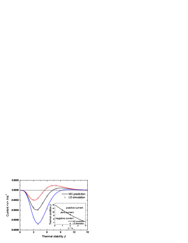
Figure 2: Temperature-driven reversal of ratchets current. Close agreement between analytical MC prediction and Langevin dynamical (LD) simulation. The simulation parameters are: $R=0.005$, $L=1.0$, $F=0.6$, $\theta=0.42$, $\gamma=1$ and $\tau_{c}=0.15,0.25,0.5$ from top to bottom. Error bars are smaller than the symbol size. Inset: extracted zero-current curve with respect to $\gamma/\tau_{c}$.

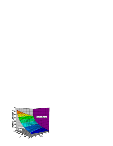
Figure 3: The zero-current surface with respect to parameters $\beta$, $\gamma/\tau_{c}$ and $F$.

Note that the analytical ratchet current in Eq. (19) is derived without the assumption of low temperature as in Reimann and Elston (1996). Additionally, the above MC method can reasonably be extended to ratchets driven by an $n$-state process or even an Ornstein-Uhlenbeck (O-U) process Risken (1967) (an O-U process is equivalent to an infinite $n$-state process from the MC point of view). With some modifications, the MC analysis can also be applied to model the temperature (generalized Smoluchowski-Feynman) ratchets Reimann (2002).

To summarize, we presented a time-quantified MC method, based on and extended from the Gambler’s Ruin problem, to analyze the directed transport in overdamped Brownian ratchets. By considering the transition probabilities and the MFPT between the adjacent minima of the periodic ratchet, we derived the analytical expression for the current in the presence of dischotomous noise, as well as the vanishing current condition. Generally, the MC formalism offers an alternative way to solve intractable stochastic dynamics and the corresponding Fokker-Planck equations. Extensions to the classic Gambler’s Ruin or other MC problems, e.g. inclusion of correlations Bohm (2000) or multiple currencies Orr and Zeilberger (1994), may yield further insights into other areas of stochastic dynamics, e.g. turbulence or high-dimensional thermally activated dynamics.

References

- Feller (1968) W. Feller, An introduction to probability theory and its applications, vol. 1 (Wiley, 1968), 3rd ed.
- Cheng et al. (2006) X. Z. Cheng, M. B. A. Jalil, H. K. Lee, and Y. Okabe, Phys. Rev. Lett. 96, 067208 (2006).
- Kikuchi et al. (1991) K. Kikuchi, M. Yoshida, T. Maekawa, and H. Watanabe, Chem. Phys. Lett. 185, 335 (1991).
- Reimann (2002) P. Reimann, Phys. Rep. 361, 57 (2002).
- Astumian and Bier (1994) R. D. Astumian and M. Bier, Phys. Rev. Lett. 72, 1766 (1994).
- Doering et al. (1994) C. R. Doering, W. Horsthemke, and J. Riordan, Phys. Rev. Lett. 72, 2984 (1994).
- Svoboda et al. (1993) K. Svoboda, C. F. Schmidt, B. J. Schnapp, and S. M. Block, Nature 365, 721 (1993).
- Kula et al. (1998) J. Kula, T. Czernik, and J. Łuczka, Phys. Rev. Lett. 80, 1377 (1998).
- Van den Broeck et al. (2004) C. Van den Broeck, R. Kawai, and P. Meurs, Phys. Rev. Lett. 93, 090601 (2004).
- Reimann and Elston (1996) P. Reimann and T. C. Elston, Phys. Rev. Lett. 77, 5328 (1996).
- Lindner et al. (1999) B. Lindner, L. Schimansky-Geier, P. Reimann, P. Hänggi, and M. Nagaoka, Phys. Rev. E 59, 1417 (1999).
- Bier and Astumian (1996) M. Bier and R. D. Astumian, Phys. Rev. Lett. 76, 4277 (1996).
- Iwaniszewski (2003) J. Iwaniszewski, Phys. Rev. E 68, 027105 (2003).
- Risken (1967) H. Risken, The Fokker-Planck Equation (Sprinter-Verlag, Berlin, 1967), 2nd ed.
- Lee et al. (2003) Y. Lee, A. Allison, D. Abbott, and H. E. Stanley, Phys. Rev. Lett. 91, 220601 (2003).
- Barik et al. (2006) D. Barik, P. K. Ghosh, and D. S. Ray, J. Stat. Mech. p. P03010 (2006).
- (17) X. Z. Cheng, M. B. A. Jalil, and H. K. Lee, to be submitted.
- Bohm (2000) W. Bohm, J. Appl. Prob. 37, 470 (2000).
- Orr and Zeilberger (1994) C. R. Orr and D. Zeilberger, J. Symbolic Comput. 18, 87 (1994).