A box-covering algorithm for fractal scaling in scale-free networks

Abstract

A random sequential box-covering algorithm recently introduced to measure the fractal dimension in scale-free networks is investigated. The algorithm contains Monte Carlo sequential steps of choosing the position of the center of each box, and thereby, vertices in preassigned boxes can divide subsequent boxes into more than one pieces, but divided boxes are counted once. We find that such box-split allowance in the algorithm is a crucial ingredient necessary to obtain the fractal scaling for fractal networks; however, it is inessential for regular lattice and conventional fractal objects embedded in the Euclidean space. Next the algorithm is viewed from the cluster-growing perspective that boxes are allowed to overlap and thereby, vertices can belong to more than one box. Then, the number of distinct boxes a vertex belongs to is distributed in a heterogeneous manner for SF fractal networks, while it is of Poisson-type for the conventional fractal objects.

A box-covering method is a basic tool to measure the fractal dimension of conventional fractal objects embedded in the Euclidean space. Such a method, however, cannot be applied to scale-free networks that exhibit an inhomogeneous degree distribution and the small-worldness. The Euclidean metric is not well defined in such networks. To check the fractality, a random sequential box-covering algorithm was recently introduced. In the algorithm, vertices within a box can be disconnected, but connected via a different box or boxes. Here we show that such box-split allowance is an essential ingredient to obtain the fractal scaling in scale-free networks, while it is inessential for the conventional fractal objects. Moreover, the algorithm is viewed from a different perspective that boxes are allowed to overlap instead of being split and thereby, vertices can belong to more than one box. Then, the number of distinct boxes a vertex belongs to is distributed in a heterogeneous manner for scale-free fractal networks, while it is of Poisson-type for the conventional fractal objects.

I Introduction

Fractal objects that are embedded in the Euclidean space have been observed in diverse phenomena feder . They contain self-similar structures within them, which are characterized in terms of non-integer dimension, i.e., the fractal dimension $d_{B}$, defined in the fractal scaling relation,

$$N_{B}(\ell_{B})\sim\ell_{B}^{-d_{B}}.$$ (1)

Here $N_{B}(\ell_{B})$ is the minimum number of boxes needed to tile a given fractal object with boxes of lateral size $\ell_{B}$. This counting method is called the box-covering method.

Fractal scaling (1) was also observed recently ss in real-world scale-free (SF) networks such as the world-wide web www , metabolic network of Escherichia coli and other microorganisms metabolic , and protein interaction network of Homo sapiens dip . SF networks ba are those that exhibit a power-law degree distribution $P_{d}(k)\sim k^{-\gamma}$. Degree $k$ is the number of edges connected to a given vertex. For such fractal networks, since their embedded space is not Euclidean, the Euclidean metric is replaced by the chemical distance.

One may define the fractal dimension in another manner through the mass-radius relation. The average number of vertices $\langle M_{C}(\ell_{C})\rangle$ within a box of lateral size $\ell_{C}$, called average box mass, scales in a power-law form,

$$\langle M_{C}(\ell_{C})\rangle\sim\ell_{C}^{d_{B}},$$ (2)

with the fractal dimension $d_{B}$. This counting method is called the cluster-growing method below. Hereafter, the subscripts $B$ and $C$ represent the box-covering and the cluster-growing methods, respectively. The formulas (1) and (2) are equivalent when the relation $N\sim N_{B}(\ell_{B})\langle M_{C}(\ell_{C})\rangle$ holds for $\ell_{B}=\ell_{C}$. Such case can be seen when fractal objects are embedded in the Euclidean space. However, for SF fractal networks, the relation (2) is replaced with the small-world behavior,

$$\langle M_{C}(\ell_{C})\rangle\sim e^{\ell_{C}/\ell_{0}},$$ (3)

where $\ell_{0}$ is a constant. Thus, the fractal scaling can be found in the box-covering method, but not in the cluster-growing method for SF fractal networks.

To understand this seemingly contradictory relations, here we investigate generic nature of the box-covering method in SF networks in comparison of the cluster-growing method. Owing to the inhomogeneity of degrees in SF fractal networks, the way of covering a network can depend on detailed rules of box-covering methods. Recently, a new box-covering algorithm was introduced by the current authors goh2006 ; jskim . In fact, this algorithm shares a common spirit with the one previously introduced by Song et al. ss , however, details differ from one another in the following perspective: Our algorithm, called random sequential (RS) box-covering method, contains a random process of selecting the position of the center of each box. A new box can overlap preceding boxes. In this case, vertices in preassigned boxes are excluded in the new box, and thereby, vertices in the new box can be disconnected within the box, but connected through a vertex (or vertices) in a preceding box (or boxes). Nevertheless, such a divided box is counted as a single one. Detailed rule is described in the next section. Such counting method is an essential ingredient to obtain the fractal scaling in fractal networks; whereas, it is inessential for regular lattice and conventional fractal objects embedded in the Euclidean space.

Next, we count how many boxes a vertex belongs to in the cluster-growing algorithm, where boxes are allowed to overlap. For the SF fractal network, the fraction of vertices counted $f$ times decays with respect to $f$ in a nontrivial manner, while for the square lattice and a conventional fractal object, it decays in a Poisson-type manner. We note that the Sierpinski gasket is used here as a fractal object embedded in the Euclidean space. Such distinct features arising in the SF fractal networks enables the coexistence of the two contradictory notions of the fractality and small-worldness.

II Random sequential box-covering

Here we describe a new box-covering method, which takes steps as follows: We start with all vertices labeled as not burned. Then,

1. Select a vertex randomly at each step; this vertex serves as a seed.

2. Search the network by distance $\ell_{B}$ from the seed and burned all vertices found but not burned yet. Assign newly burned vertices to the new box. If no newly burned vertex is found, the box is discarded.

3. Repeat (i) and (ii) until all vertices are assigned to their respective boxes.

Figure 1: (Color online) Schematic illustration of the RS box-covering algorithm introduced goh2006 ; jskim . Vertices are selected randomly, for example, from vertex 1 to 4 successively. Vertices within distance $\ell_{B}=1$ from vertex 1 are assigned to a box represented by solid (red) circle. Vertices from vertex 2, not yet assigned to their respective box are represented by dashed-doted-doted (black) closed curve, vertices from vertex 3 are represented by dashed-doted (green) circle and vertices from vertex 4 are represented by dashed (blue) ellipse.

The above method is schematically illustrated in Fig. 1. A different Monte Carlo realization of this procedure ((i)–(iii)) may yield a different number of boxes for covering the network. In this study, for simplicity, we choose the smallest number of boxes among all the trials. To obtain the power-law behavior of the fractal scaling, we needed at most ${\mathcal{O}}(10)$ Monte Carlo trials for all fractal networks we study. It should be noted that the box number $N_{B}$ we employ is not the minimum number among all the possible tiling configurations. Finding the actual minimum number over all configurations is a challenging task, which could not be reached by the Monte Carlo method.

To check the validity of our algorithm, we first apply our method to the two dimensional regular lattice in Fig. 2. While our method may perform inefficiently in the highly regular structure due to the step in which already box-assigned vertices can be selected as seeds, taking about a few hours of cpu time for system size $N=500\times 500$, we find that our method can still yield the correct dimension $\approx$2.0 for the two dimensional square lattice, as shown in Fig. 2. We also show that the number of Monte Carlo trials is not crucial to obtain the fractal scaling.

Figure 2: (Color online) Fractal scaling analysis for the two dimensional square lattice with the box-covering algorithm. Shown are the result of one Monte Carlo trial ($\circ$) and that obtained from 20 Monte Carlo trials ($\square$). From the least-square-fit of the data (straight line), the fractal dimension is measured to be $\approx$2.0 as expected.

Figure 3: (Color online) A fractal object, the Sierpinski gasket with the second generation (a). Conventional box covering based on the Euclidean metric with size $\ell_{E}=2$ (b) and $\ell_{E}=1$ (c). Box covering based on chemical distance $\ell_{B}=1$ by using the RS box-covering method (d). Seed vertices $1\to 5$ are selected successively.

Figure 4: (Color online)Fractal dimension of the Sierpinski gasket with the 12th generation measured by using the RS box-covering method. Solid line is guideline with slope $-\ln 3/\ln 2$. Shown are the result of one Monte Carlo trial ($\circ$) and that obtained from 20 Monte Carlo trials ($\square$).

Fig.3 shows the box-covering method applied to the Sierpinski gasket with the third generation (a). One can find easily that $N_{B}(\ell_{E}=2)=3$ in (b) and $N_{B}(\ell_{E}=1)=9$ in (c) when lateral size $\ell_{E}$ is taken as the conventional Euclidean metric. The obtained $N_{B}(\ell_{E})$ are the minimum numbers of boxes needed to tile the object for each case. In Fig.3(d), we show a configuration in box-covering ensemble obtained from our current algorithm with distance $\ell_{B}=1$. One can see that $N_{B}(\ell_{B})$ can vary depending on Monte Carlo trials. We show, however, that the fractal dimension is obtained by using the conventional method in (b) and (c), $d_{B}=-\ln 3/\ln 2$. Numerical value is obtained from the Sierpinski gasket with the 12th generation, composed of 265,721 vertices, and the fractal scaling is shown in Fig. 4.

Our algorithm also generates the same fractal dimensions for SF fractal networks such as the world-wide web, the metabolic network of E. coli, the protein interaction networks of H. sapiens and S. cerevisiae as obtained by Song et al. ss . Fig.5 shows the fractal scaling for the world-wide web, displaying the same fractal dimension $d_{B}\approx 4.1$. In comparison of the method by Song et al., ours is easier to implement, because it does not contain the procedure for constraining the maximum separation within a box and is carried out in random sequential manner in box covering.

Figure 5: (Color online) Comparison of the box-covering methods introduced by Song et al. ss ($\square$) and in this paper ($\circ$) for the world-wide web. The results obtained from the two box-covering methods applied to the world-wide web are plotted here. The two methods yield the same fractal dimension $d_{B}\approx 4.1$. The method introduced by Song et al. is more optimal than ours in the viewpoint that $N_{B}(\ell_{S})<N_{B}(2\ell_{B}+1)$.

Figure 6: (Color online) Fractal scaling analysis for the world-wide web by the two box-covering algorithms, that of Song et al. ($\square$) and of ours ($\circ$). For comparison, the horizontal scale for that of Song et al. is rescaled as $\ell_{S}/1.5\to\ell_{B}$, by which we get the overlap of two curves obtained from the different algorithms.

The particular definition of box size has proved to be inessential for fractal scaling. It is rather inappropriate to compare the length scale $\ell_{B}$ with that $\ell_{S}$ used in Ref. ss , because the two methods involve different definitions of the boxes. What is interesting, however, is that there exists a linear relationship, for example $\ell_{S}/1.5\to\ell_{B}$ in the case of the world-wide web as shown in Fig. 6. This linear relationship indicates that despite the difference in the two algorithms, such a difference does not lead to qualitatively different fractal-scaling behaviors.

III Overlap of box covering and vertices disconnectedness

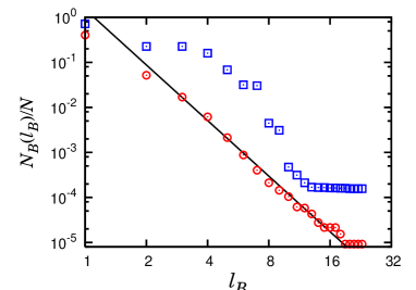
Figure 7: (Color online) Fractal scaling analysis for the world-wide web with the RS box-covering algorithm ($\circ$) and its variant that disallows disconnected boxes ($\square$)

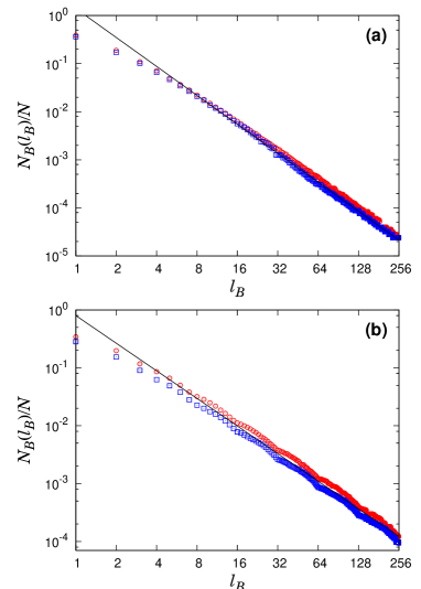
Figure 8: (Color online) Fractal scaling analysis for the square lattice (a) and the Sierpinski gasket (b) with the RS box-covering algorithm ($\circ$) and its variant that disallows disconnected boxes ($\square$). Solid lines are guidelines with slopes of $-2$ in (a) and $-\ln 3/\ln 2$ in (b).

It is interesting to note that in our algorithm vertices can be disconnected within a box, but connected through a vertex (or vertices) in a different box (or boxes) as in the case of box 2 shown in Fig. 1. On the other hand, if we construct a box with only connected vertices, for example, box 2 is regarded as two separate boxes, then the power-law behavior Eq. (1) is not observed for the world-wide web as shown in Fig. 7. We check if such difference appears even for a regular lattice and a fractal object embedded in the Euclidean space. Figs. 8 show that such different behavior does not occur for the square lattice in two dimensions and the Sierpinski gasket. We show that such fact originates from the inhomogeneity of degrees in SF networks as follows: Owing to their large degree, hub vertices can be assigned to boxes earlier than other vertices when their neighbors are selected as seeds of boxes. Once hub vertices are assigned to one of the boxes, they can make subsequent boxes disconnected when vertices in those boxes are connected via hub vertices. Box 2 in Fig. 1 is such a case. In SF networks, such cases occur at a non-negligible rate.

To study the fraction of disconnected boxes quantitatively, we invoke the cluster-growing approach. In this approach, boxes are allowed to overlap, and thereby, a vertex can belong to more than one box. Thus, the extent of overlap of the boxes during the tiling can provide important information on the fraction of disconnected boxes in the box-covering method. In this regard, we reported the cumulative fraction $F_{c}(f)$ of vertices counted $f$ times or more in the cluster-growing method for the world-wide web in jskim and is reproduced in Fig. 9. The cumulative fraction $F_{c}(f)$ is likely to follow a power law for small $f$, thereby indicating that the overlaps occur in a non-negligible frequency even for a small distance $\ell_{C}$. The associated exponent decreases with increase in box size $\ell_{C}$ as the chances of overlaps increase. However, for large values of $f$, the large fraction of vertices counted exceed the frequency extrapolated from the power-law behavior. For the square lattice and the Sierpinski gasket, however, the fraction $F(f)$ follows a bounded distribution with a peak at small $f$ as shown in Fig. 10. Thus, for the fractal networks like the world-wide web, there are a significant number of vertices that are counted quite a few times in the cluster-growing method, but such vertices are extremely rare in the conventional fractal objects such as the Sierpinski gasket. Such multiple counting due to overlap is excluded in the box-covering method. This exclusion effect makes the average mass of a box in the box-covering method significantly lower than that in the cluster-growing method.

Figure 9: (Color online) Cumulative fraction $F_{c}(f)$ of the vertices counted $f$ times in the cluster-growing algorithm. $F_{c}(f)$ follows a power law in the small $f$ region, where the slope depends on box size $\ell_{C}$. However, for large values of $f$, the data largely deviate from the value extrapolated from the power-law behavior. Data are presented for $\ell_{C}=2$ ($\bullet$), $\ell_{C}=3$ ($\blacksquare$), and $\ell_{C}=5$ ($\blacktriangle$).

Figure 10: (Color online) Fraction $F(f)$ of the vertices counted $f$ times in the cluster-growing algorithm for the Sierpinski gasket with the 12th generation composed of 265,721 vertices. $F(f)$ follows a Poisson-type distribution. Data are presented for $\ell_{C}=2$ ($\bullet$), $\ell_{C}=3$ ($\blacksquare$), and $\ell_{C}=5$ ($\blacktriangle$).

Next, one may wonder if the RS box-covering algorithm can be improved in efficiency by excluding already-burned vertices from the list of the root candidates of new boxes. In Fig. 11, we compare the fractal scaling behaviors obtained from the two cases of keeping or excluding already-burned vertices from the list for two networks: the world-wide web (a) and the fractal model introduced in goh2006 . We find that the two cases exhibit somewhat different behaviors. If the already-burned vertices are excluded from the next selection, the power-law behavior is not obtained for the world-wide web. However, they exhibit similar power-law behaviors for the fractal model, even though the two data sets show somewhat deviations.

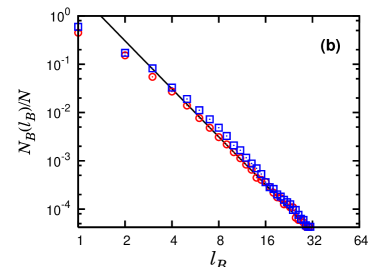
Figure 11: (Color online) Fractal scaling analysis with the rules that allow ($\circ$) or disallow ($\square$) the already-box-burned vertices to be chosen as the roots of new boxes for the world-wide web (a), and the fractal model (b).

IV Conclusions and Discussion

We have studied various features of the random sequential box-covering algorithm by applying it to a SF fractal network, the world-wide web, and a regular and a conventional fractal object, the square lattice and the Sierpinski gasket, respectively. Results obtained from the two classes of networks exhibit distinct feature. The condition that vertices in a box can be disconnected in the box-covering method turns out to be an essential ingredient to have the fractal scaling for a SF fractal network, however, it is irrelevant for a regular lattice and a conventional fractal object embedded in the Euclidean space. We also found that the fraction of vertices counted $f$ times in the cluster-growing method exhibits a non-trivial behavior for the former, while it does a trivial behavior for the latter. The two results are complementary; thereby, the SF fractal network exhibits the fractal scaling (1) in the box-covering and the small-world behavior (3) in the cluster-growing method. Finally, it is noteworthy that our box-covering algorithm is a modification of the algorithm used in the random sequential packing problem packing .

This work was supported by KRF Grant No. R14-2002-059-010000-0 of the ABRL program funded by the Korean government (MOEHRD). Notre Dame’s Center for Complex Networks kindly acknowledges the support of the National Science Foundation under Grant No. ITR DMR-0426737.

References

- (1) J. Feder, Fractals (Plenum, New York, 1988).
- (2) C. Song, S. Havlin, and H.A. Makse, Nature (London) 433, 392 (2005).
- (3) R. Albert, H. Jeong, and A.-L. Barabási, Nature (London) 401, 130 (1999).
- (4) H. Jeong, B. Tombor, R. Albert, Z.N. Oltvai, and A.-L. Barabási, Nature (London) 407, 651 (2000).
- (5) I. Xenarious, et al. Nucleic Acids Res. 28, 289 (2000).
- (6) A.-L. Barabási and R. Albert, Science 286, 509 (1999).
- (7) K.-I. Goh, G. Salvi, B. Kahng and D. Kim, Phys. Rev. Lett. 96, 018701 (2006).
- (8) J.S. Kim, K.-I. Goh, G. Salvi, E. Oh, B. Kahng, and D. Kim, to appear in Phys. Rev. E.
- (9) M. Nakamura, J. Phys. A. 19, 2345 (1986); J.W. Evans, ibid 20, 3063 (1987).