Complex permittivity of a biased superlattice

Abstract

Intersubband response in a superlattice subjected to a homogeneous electric field (biased superlattice with equipopulated levels) is studied within the tight-binding approximation, taking into account the interplay between homogeneous and inhomogeneous mechanisms of broadening. The complex dielectric permittivity is calculated beyond the Born approximation for a wide spectral region and a low-frequency enhancement of the response is found. A detectable gain below the resonance is obtained for the low-doped $GaAs$-based biased superlattice in the THz spectral region. Conditions of the stimulated emission regime for metallic and dielectric waveguide structures are discussed. The appearence of a localized THz mode due to BSL placed at the interface vacuum-dielectric is described.

I Introduction

The mechanisms of the stimulated emission due to intersubband transitions of electrons in different tunnel-coupled structures (monopolar laser effect) have been investigated during the previous decade (see Refs. in 1 ; 2 ). As a result, both mid-IR and THz lasers viability has been demonstrated with the use of the scheme based on the vertical transport through quantum cascade structures, which incorporate injector and active regions. Since a population inversion appears in the active region, the stimulated emission occurs for the mode propagated along mid-IR or THz waveguide.

In the case of a biased superlattice (BSL), the vertical current through the Wannier-Stark ladder, which takes place under the condition $2T\ll\varepsilon_{\scriptscriptstyle B}$ (here $\varepsilon_{\scriptscriptstyle B}/\hbar$ is the Bloch frequency and $T$ stands for the tunneling matrix element between adjacent quantum wells (QWs) 3 ; 4 ), does not change level populations. Thus, the consideration based on the golden rule approach gives zero absorption. In contrast to this, for the wide miniband BSL, with the bandwidth $2T\gg\varepsilon_{\scriptscriptstyle B}$, a negative differential conductivity, i.e. gain due to Bloch oscillations, was studied theoretically starting the 70s 5 (see further results and references in 6 ) and demonstrated in recent experiments 7 ; 8 . At the same time, a similar behavior of the THz response, including a crossover from gain to absorption regime with detuning energy shifted through the resonance, was reported for the BSL with tight-binding electronic states 9 . This contradiction with the simple quantum picture, where a zero response should take place, and the question about THz gain without inversion beyond the Born approximation are discussed in 10 ; 11 . To the best of our knowledge, the consideration of the response of a tight-binding BSL is not performed yet in spite of both real and imaginary contributions to the dielectric permittivity, $\Delta\epsilon_{\omega}$, appear to be essential for wide miniband BSLs 6 ; 8 .

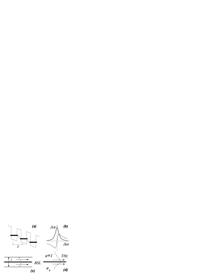
Figure 1: Transitions between broaded levels in BSL of period $Z$ with the Wannie-Stark ladder $(a)$. Peak and dispersive contributions of these transitions to the dielectric permittivity, $\Delta\epsilon_{\omega}$ (solid and dashed curves are correspondent to $Re(\Delta\epsilon_{\omega})$ and $Im(\Delta\epsilon_{\omega})$ respectively) $(b)$. Geometries of the THz waveguides with the BSL placed between the ideal metallic mirrors $(c)$, and at the interface vacuum-dielectric $(d)$.

In this paper, we evaluate the response of a BSL placed on a high-frequency electric field taking into account both homogeneous and inhomogeneous mechanisms of broadening exactly. Within the tight-binding approach, which corresponds to the sequential tunneling picture (Fig. 1$a$), we analyze the frequency dispersion of complex dielectric permittivity (Fig. 1$b$). The Green’s function formalism is used to describe both homogeneous and inhomogeneous mechanisms of broadening, and the quasi-equilibrium distribution of electrons over tunnel-coupled wells. We demonstrate the low-frequency enhancement of the response under consideration. Further, the propagation of the transverse magnetic (TM) mode along THz waveguides with the BSL placed between ideal metallic mirrors (Fig. 1$c$) and at the interface vacuum-dielectric (Fig. 1$d$) is considered. The appearance of a localized mode is founded for the second case. We also discuss the conditions for the stimulated emission regime for the two cases under consideration.

The paper is organized as follows. In the next section we consider the THz response of BSL and in Sec. III we discuss the spectral dependencies of dielectric permittivity, while in Sec. IV we consider the mode propagation for the BSL placed in the THz waveguide. The last section includes a discussion of the approximations used and conclusions.

II Basic Equations

Within the framework of the tight-binding approach we describe the electronic states in BSL using the in-plane inhomogeneous matrix Hamiltonian $\hat{h}_{rr^{\prime}}$ and the non-diagonal perturbation matrix due to a transverse field $[E_{\scriptscriptstyle\bot}\exp(-i\omega t)+c.c.]$ written as $[\widehat{\delta h}_{rr^{\prime}}\exp(-i\omega t)+H.c.]$:

$$\hat{h}_{rr^{\prime}} = \left(\frac{\hat{p}^{2}}{2m}+V_{r\mathbf{x}}+r\varepsilon_{\scriptscriptstyle B}\right)\delta_{rr^{\prime}}+T(\delta_{rr^{\prime}-1}+\delta_{rr^{\prime}+1}),$$

$$\widehat{\delta h}_{rr^{\prime}} = \frac{ev_{\scriptscriptstyle\bot}}{\omega}E_{\scriptscriptstyle\bot}(r-r^{\prime})(\delta_{rr^{\prime}-1}+\delta_{rr^{\prime}+1}).~{}~{}~{}~{}~{}~{}$$ (1)

Here $r=0,\pm 1,\ldots$ stands as a QW number, $\hat{p}^{2}/2m$ is the in-plane kinetic energy operator, and $m$ is the effective mass. The random potential energy of the $r$-th QW, $V_{r\mathbf{x}}$, is statistically independent in each QW and includes both short- and long-scale parts of potential. The Bloch energy, $\varepsilon_{\scriptscriptstyle B}\simeq|e|FZ$, appears in (1) due to the shift of levels in the SL with period $Z$ under a homogeneous electric field $F$, and $v_{\scriptscriptstyle\bot}=TZ/\hbar$ stands for the transverse velocity 12 . The high-frequency current density, $[I_{\omega}\exp(-i\omega t)+c.c.]$, which involves $\propto\omega^{-1}$ response and the intersubband contribution induced by the perturbation $\widehat{\delta h}_{rr^{\prime}}$, is determined by:

$$I_{\omega}=i\frac{e^{2}n}{m\omega}E_{\scriptscriptstyle\bot}+i\frac{2ev_{\scriptscriptstyle\bot}}{L^{3}}\left\langle\left\langle\sum_{r}\mathrm{sp}_{\scriptscriptstyle\|}(\widehat{\delta\rho}_{r+1r}-\widehat{\delta\rho}_{r-1r})\right\rangle\right\rangle,$$ (2)

where $n$ is the electron concentration, factor 2 is due to spin, $\mathrm{sp}_{\scriptscriptstyle\|}\ldots$ is the trace over in-plane motion, $\langle\langle\ldots\rangle\rangle$ is the averaging over random potentials $V_{r\mathbf{x}}$, and $L^{3}$ is the normalization volume.

The high-frequency contribution to the density matrix in Eq. (2), $[\widehat{\delta\rho}_{rr^{\prime}}\exp(-i\omega t)+H.c.]$, is governed by the independent linearized equations for $\widehat{\delta\rho}_{r}^{\scriptscriptstyle(\pm)}\equiv\widehat{\delta\rho}_{r\pm 1r}$, see 11 ; 13 :

$$-i\omega\widehat{\delta\rho}_{r}^{\scriptscriptstyle(\pm)}+\frac{i}{\hbar}(\hat{h}_{r\pm 1}\widehat{\delta\rho}_{r}^{\scriptscriptstyle(\pm)}-\widehat{\delta\rho}_{r}^{\scriptscriptstyle(\pm)}\hat{h}_{r})$$ (3)

$$\simeq \pm i\frac{ev_{\scriptscriptstyle\bot}}{\hbar\omega}E_{\scriptscriptstyle\bot}(\hat{\rho}_{r\pm 1}-\hat{\rho}_{r})$$

with the in-plane Hamiltonian of the $r$-th QW written in the form $\hat{h}_{r}=\hat{p}^{2}/2m+V_{r\mathbf{x}}+r\varepsilon_{\scriptscriptstyle B}$. Here we restrict ourselves to the consideration of only $\propto T^{2}$ contributions and the steady-state density matrix is written as $(\hat{\rho}_{o})_{rr^{\prime}}\simeq\delta_{rr^{\prime}}\hat{\rho}_{r}$. Next, we describe the electron states in the $r$-th QW by the use of the eigenstate problem $(\hat{p}^{2}/2m+V_{r\mathbf{x}})\psi_{r\mathbf{x}}^{\nu}=\varepsilon_{r\nu}\psi_{r\mathbf{x}}^{\nu}$, where the quantum number $\nu$ marks an in-plane state. Using this basis, we transform Eq. (3) into the form:

$$(\varepsilon_{r\pm 1\nu}-\varepsilon_{r\nu^{\prime}}\pm\varepsilon_{\scriptscriptstyle B}-\hbar\omega-i\lambda)\delta\rho_{r}^{\scriptscriptstyle(\pm)}(\nu,\nu^{\prime})$$

$$=\pm\frac{ev_{\scriptscriptstyle\bot}}{\omega}E_{\scriptscriptstyle\bot}[f_{\varepsilon_{r\pm 1\nu}}-f_{\varepsilon_{r\nu^{\prime}}}]\int d\mathbf{x}\psi_{r\pm 1\mathbf{x}}^{\nu}\psi_{r\mathbf{x}}^{\nu^{\prime}~{}\ast}.$$ (4)

Here $\lambda\rightarrow+0$ and we apply the quasi-equilibrium distribution of $r-$th QW, $\hat{\rho}_{r}=f_{\hat{p}^{2}/2m+V_{r\mathbf{x}}}$, where $f_{\varepsilon}$ is the Fermi function with chemical potentials $\mu$, and temperatures $T_{e}$, which are identical for any QW.

The current density (2) is given by

$$I_{\omega}\simeq i\frac{e^{2}n}{m\omega}E_{\scriptscriptstyle\bot}+i\frac{2ev_{\scriptscriptstyle\bot}}{L^{3}}\left\langle\left\langle\sum_{r\nu\nu^{\prime}}\left[\delta\rho_{r}^{\scriptscriptstyle(+)}(\nu,\nu^{\prime})\right.\right.\right.~{}~{}~{}~{}~{}~{}$$ (5)

$$\left.\left.\left.\times\int d\mathbf{x}\psi_{r+1\mathbf{x}}^{\nu~{}\ast}\psi_{r\mathbf{x}}^{\nu^{\prime}}-\delta\rho_{r}^{\scriptscriptstyle(-)}(\nu,\nu^{\prime})\int d\mathbf{x}\psi_{r-1\mathbf{x}}^{\nu~{}\ast}\psi_{r\mathbf{x}}^{\nu^{\prime}}\right]\right\rangle\right\rangle$$

and the transverse conductivity, $\sigma_{\omega}^{\scriptscriptstyle\bot}$, introduced according to the standard formula $I_{\omega}=\sigma_{\omega}^{\scriptscriptstyle\bot}E_{\scriptscriptstyle\bot}$, takes the form:

$$\sigma_{\omega}^{\scriptscriptstyle\bot} = i\frac{e^{2}n}{m\omega}+i\frac{2(ev_{\scriptscriptstyle\bot})^{2}}{\omega L^{3}}\left\langle\left\langle\sum_{r\nu\nu^{\prime}}(f_{\varepsilon_{r+1\nu}}-f_{\varepsilon_{r\nu^{\prime}}})\right.\right.$$

$$\times Q_{r+1,r}^{\nu\nu^{\prime}}\left[\frac{1}{\varepsilon_{r+1\nu}-\varepsilon_{r\nu^{\prime}}+\varepsilon_{\scriptscriptstyle B}-\hbar\omega-i\lambda}\right.$$

$$\left.\left.\left.+\frac{1}{\varepsilon_{r+1\nu}-\varepsilon_{r\nu^{\prime}}+\varepsilon_{\scriptscriptstyle B}+\hbar\omega+i\lambda}\right]\right\rangle\right\rangle,$$

where $Q_{r,r^{\prime}}^{\nu\nu^{\prime}}=\left|\int d\mathbf{x}\psi_{r\mathbf{x}}^{\nu~{}\ast}\psi_{r^{\prime}\mathbf{x}}^{\nu^{\prime}}\right|^{2}$ is the overlap factor. We have replaced $r\rightarrow r+1,\nu\leftrightarrow\nu^{\prime}$ in the second addendum. In order to check the non-singular behavior of $\sigma_{\omega}$ at $\omega\rightarrow 0$, one has to utilize the relation

$$\frac{n}{m}+\frac{2v_{\scriptscriptstyle\bot}^{2}}{L^{3}}\sum_{r\nu\nu^{\prime}}Q_{r+1,r}^{\nu\nu^{\prime}}\frac{f_{\varepsilon_{r+1\nu}}-f_{\varepsilon_{r\nu^{\prime}}}}{\varepsilon_{r+1\nu}-\varepsilon_{r\nu^{\prime}}+\varepsilon_{\scriptscriptstyle B}}=0,$$ (7)

which can be proofed with the use of the definition $n=2\sum_{r\nu}f_{\varepsilon_{r\nu}}$ and the relation $v_{\scriptscriptstyle\bot}^{2}Q_{r,r^{\prime}}^{\nu\nu^{\prime}}=|\langle r\nu|\hat{v}_{z}|r^{\prime}\nu^{\prime}\rangle|^{2}$, see 13A . Using (7) we obtain the transverse dielectric permittivity, $\epsilon_{\omega}^{\scriptscriptstyle\bot}=\epsilon+i4\pi\sigma_{\omega}^{\scriptscriptstyle\bot}/\omega$, in the form:

$$\epsilon_{\omega}^{\scriptscriptstyle\bot}=\epsilon+\frac{2\pi(2ev_{\scriptscriptstyle\bot})^{2}}{\omega^{2}L^{3}}\left\langle\left\langle\sum_{r\nu\nu^{\prime}}Q_{r+1,r}^{\nu\nu^{\prime}}(f_{\varepsilon_{r+1\nu}}-f_{\varepsilon_{r\nu^{\prime}}})\right.\right.$$

$$\times\left[\frac{2}{\varepsilon_{r+1\nu}-\varepsilon_{r\nu^{\prime}}+\varepsilon_{\scriptscriptstyle B}}-\frac{1}{\varepsilon_{r+1\nu}-\varepsilon_{r\nu^{\prime}}+\varepsilon_{\scriptscriptstyle B}-\hbar\omega-i\lambda}\right.$$

$$\left.\left.\left.-\frac{1}{\varepsilon_{r+1\nu}-\varepsilon_{r\nu^{\prime}}+\varepsilon_{\scriptscriptstyle B}+\hbar\omega+i\lambda}\right]\right\rangle\right\rangle~{}~{}~{}~{}~{}~{}$$ (8)

and intersubband transitions give a finite contribution to (8) in the static limit. Finally, we transform 14 the denominators in (8) and rewrite $\Delta\epsilon_{\omega}^{\scriptscriptstyle\bot}=\epsilon_{\omega}^{\scriptscriptstyle\bot}-\epsilon$ through the spectral density function 13 ; 15 , $\mathcal{A}_{r,\varepsilon}(\mathbf{x},\mathbf{x^{\prime}})=\sum_{\nu}\psi_{r\mathbf{x}}^{\nu}\psi_{r\mathbf{x}^{\prime}}^{\nu~{}\ast}\delta(\varepsilon-\varepsilon_{r\nu})$, in the following form

$$\Delta\epsilon_{\omega}^{\scriptscriptstyle\bot}=\frac{2\pi(2ev_{\scriptscriptstyle\bot})^{2}}{\omega^{2}L^{3}}\int_{-\infty}^{\infty}d\varepsilon\int_{-\infty}^{\infty}d\varepsilon^{\prime}(f_{\varepsilon}-f_{\varepsilon^{\prime}})\left[\frac{2}{\varepsilon-\varepsilon^{\prime}+\varepsilon_{\scriptscriptstyle B}}\right.$$

$$\left.-(\varepsilon-\varepsilon^{\prime}-\Delta\varepsilon_{-}-i\lambda)^{-1}-(\varepsilon-\varepsilon^{\prime}+\Delta\varepsilon_{+}+i\lambda)^{-1}\right]~{}~{}~{}~{}~{}~{}$$

$$\times\int d\mathbf{x}\int d\mathbf{x^{\prime}}~{}\sum_{r}\langle\langle\mathcal{A}_{r+1,\varepsilon}(\mathbf{x},\mathbf{x^{\prime}})\mathcal{A}_{r,\varepsilon^{\prime}}(\mathbf{x^{\prime}},\mathbf{x})\rangle\rangle~{}~{}~{}~{}$$ (9)

with $\Delta\varepsilon_{\pm}=\hbar\omega\pm\varepsilon_{\scriptscriptstyle B}$. Thus, we have evaluated the expression for the transverse response taking into account the scattering processes exactly.

Further, we perform the averaging over short-range and large-scale potentials in the last factor, keeping in mind that the averaged characteristics of scattering processes, both for homogeneous and inhomogeneous mechanisms, do not dependent on the QW number $r$. Following Eqs. (11 - 13) of Ref. 11 we obtain

$$\int\int\frac{d\mathbf{x}d\mathbf{x^{\prime}}}{L^{3}}\sum_{r}\langle\langle\mathcal{A}_{r+1,\varepsilon}(\mathbf{x},\mathbf{x^{\prime}})\mathcal{A}_{r,\varepsilon^{\prime}}(\mathbf{x^{\prime}},\mathbf{x})\rangle\rangle$$ (10)

$$= \frac{\rho_{\scriptscriptstyle 2D}}{2Z}\int_{0}^{\infty}d\xi A(\xi-\varepsilon)A(\xi-\varepsilon^{\prime}),$$

where the averaged spectral density, $A(E)$, is written in the integral form:

$$A(E)=\int_{-\infty}^{0}\frac{dt}{\pi\hbar}\cos\left(\frac{Et}{\hbar}\right)e^{\gamma t/\hbar-(\Gamma t/\hbar)^{2}/2}.$$ (11)

Here $\Gamma=\sqrt{\langle w_{r\mathbf{x}}^{2}\rangle}$ is the inhomogeneous broadening energy due to the large-scale part of the potential in the $r$-th QW, $w_{r\mathbf{x}}$, and $\gamma$ stands for the homogeneous broadening energy. In (11) we consider the case of scattering by zero-radius centers when $\gamma$ does not depend on $\varepsilon$, $p$ or $\mathbf{x}$ and the shift of levels, which is logarithmically divergent without a small-distance cutoff 16 , is included into the zero point energy. The simple analytical expressions for the spectral density peak take the form in the limiting cases:

$$A(E)=\left\{\begin{array}[]{cc}\gamma/[\pi(E^{2}+\gamma^{2})],&\Gamma=0\\ \exp(-E^{2}/2\Gamma^{2})/(\sqrt{2\pi}\Gamma),&\gamma=0\end{array}\right.$$ (12)

and $A(E)$ transforms from a Lorentzian towards a Gaussian line shape upon an increase in the contribution of the inhomogeneous broadening.

According to Eqs. (9, 10), one needs to consider the convolution of spectral densities, $D(\varepsilon,\varepsilon^{\prime})=\int_{0}^{\infty}d\xi A(\xi-\varepsilon)A(\xi-\varepsilon^{\prime})$. For the collisionless case, when (12) is replaced by the $\delta$-function, one should replace $D(\varepsilon,\varepsilon^{\prime})$ by $\theta(\varepsilon+\varepsilon^{\prime})\delta(\varepsilon-\varepsilon^{\prime})$. Modifications of $D(\varepsilon,\varepsilon^{\prime})$ due to broadening are shown in Fig. 2 for the cases $\gamma=\Gamma$ and $\gamma=3\Gamma$. Using the variables $\varepsilon-\varepsilon^{\prime}$ and $(\varepsilon+\varepsilon^{\prime})/2$ we obtain $D(\varepsilon,\varepsilon^{\prime})$ as a peak of width of the order of broadening with respect to $\varepsilon-\varepsilon^{\prime}$ and $D(\varepsilon,\varepsilon^{\prime})$ is suppressed at negative $(\varepsilon+\varepsilon^{\prime})/2$ 17 . Note that tails of peaks are suppressed if the inhomogeneous contribution increases.

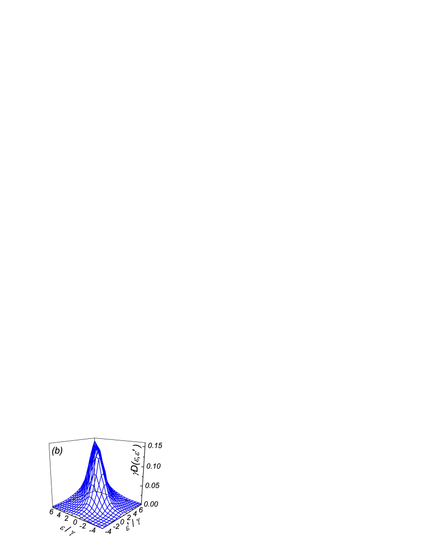
Figure 2: (Color online) Dimensionless convolution of spectral densities, $\gamma D(\varepsilon,\varepsilon^{\prime})$, plotted for $\gamma=\Gamma$ $(a)$, and $\gamma=3$ $\Gamma$ $(b)$.

III Frequency Dispersion

Here we consider the frequency dispersion of dielectric permittivity tensor $\epsilon_{\omega}^{\scriptscriptstyle\|,\bot}$. The in-plane component of permittivity, $\epsilon_{\omega}^{\scriptscriptstyle\|}$, is written through the Drude conductivity $\sigma_{\omega}^{\scriptscriptstyle\|}=ie^{2}n/m(\omega+i\gamma/\hbar)$ in the form:

$$\epsilon_{\omega}^{\scriptscriptstyle\|}=\epsilon-\frac{4\pi e^{2}n}{m\omega(\omega+i\gamma/\hbar)}$$ (13)

with the homogeneous relaxation frequency, $\gamma/\hbar$, introduced in Sec. II. The transverse component is given by Eq. (9), which can be written through $D(\varepsilon,\varepsilon^{\prime})$ and the 2D density of states, $\rho_{\scriptscriptstyle 2D}$, as follows:

$$\Delta\epsilon_{\omega}^{\scriptscriptstyle\bot}=\frac{\pi(2ev_{\scriptscriptstyle\bot})^{2}}{\omega^{2}Z}\rho_{\scriptscriptstyle 2D}\int_{-\infty}^{\infty}d\varepsilon\int_{-\infty}^{\infty}d\varepsilon^{\prime}~{}~{}~{}~{}~{}~{}~{}~{}$$

$$\times D(\varepsilon,\varepsilon^{\prime})(f_{\varepsilon^{\prime}}-f_{\varepsilon})\left[2/(\varepsilon-\varepsilon^{\prime}+\varepsilon_{\scriptscriptstyle B})\right.~{}~{}~{}~{}~{}~{}~{}$$ (14)

$$\left.-(\varepsilon-\varepsilon^{\prime}-\Delta\varepsilon_{-}-i\lambda)^{-1}-(\varepsilon-\varepsilon^{\prime}+\Delta\varepsilon_{+}+i\lambda)^{-1}\right].~{}~{}~{}$$

The Fermi distribution, $f_{\varepsilon}$, is connected to the averaged concentration, $n_{\scriptscriptstyle 2D}=nZ$, according to the standard relation $n_{\scriptscriptstyle 2D}=\int_{-\infty}^{\infty}d\varepsilon f_{\varepsilon}\rho_{\varepsilon}=\rho_{\scriptscriptstyle 2D}\int_{-\infty}^{\infty}d\varepsilon f_{\varepsilon}\int_{0}^{\infty}d\xi A(\xi-\varepsilon)$, where $\rho_{\varepsilon}$ is written through $A(E)$ given by Eq. (11).

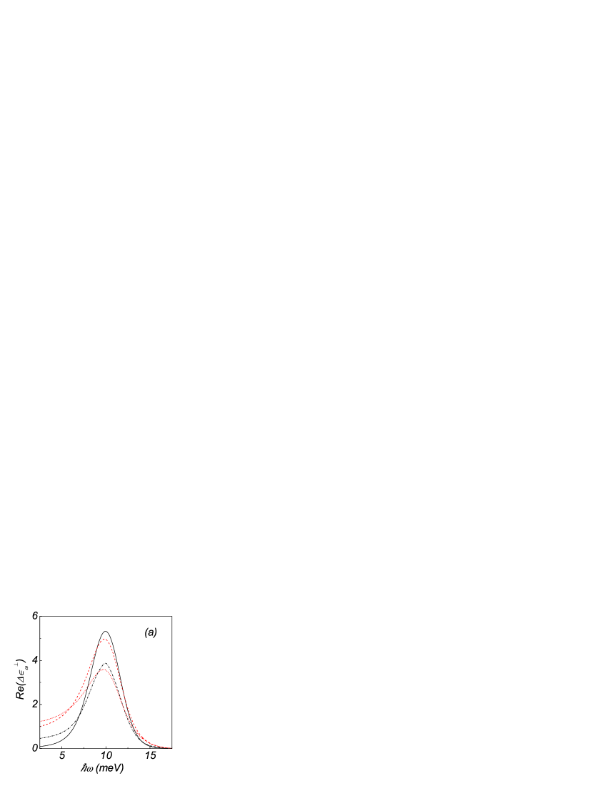
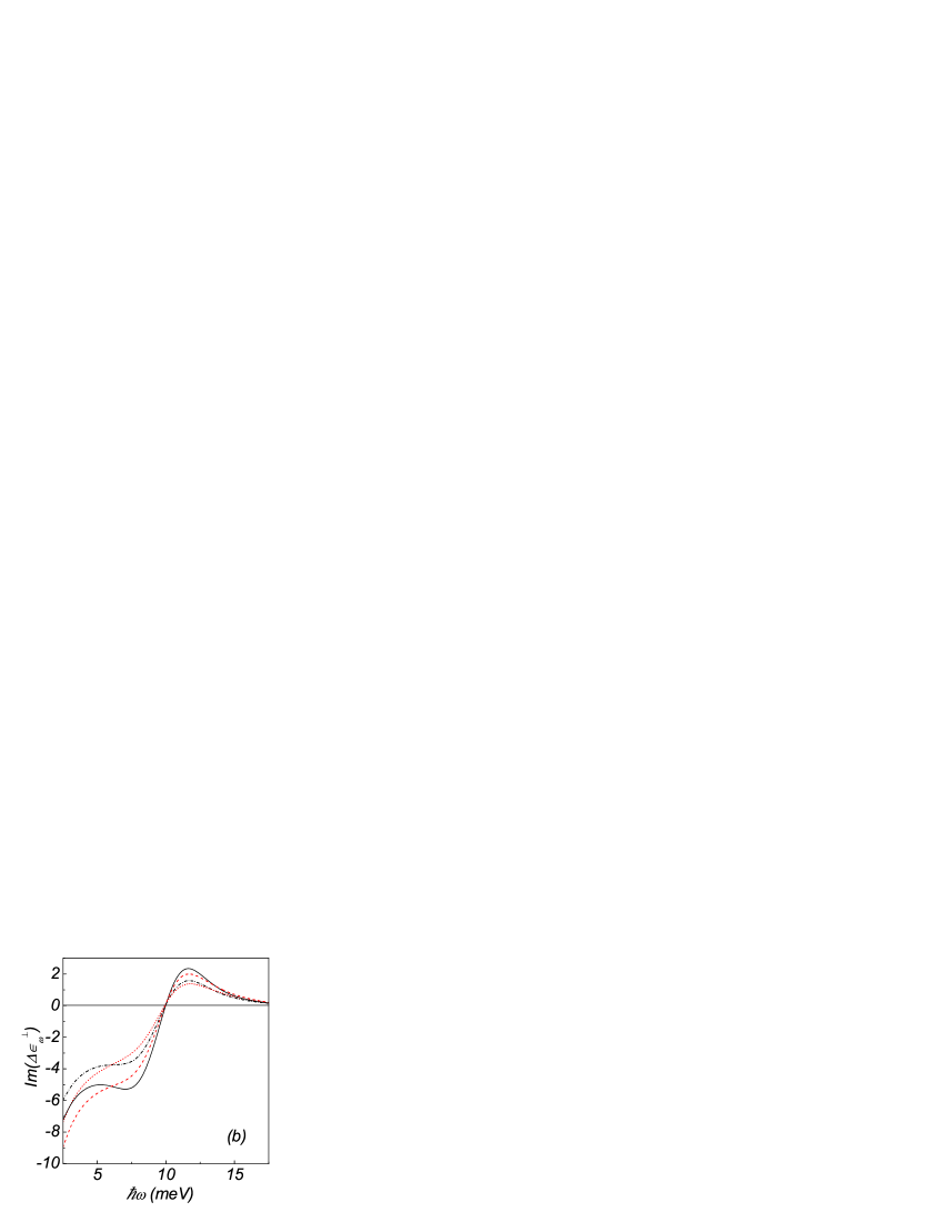
Figure 3: (Color online) Frequency dispersion of the real ($a$) imaginary ($b$) parts of dielectric permittivity $\Delta\epsilon_{\omega}^{\perp}$ . For the case $\gamma=\Gamma=0.8$ meV one uses $\mu=1.5$ meV, $T_{e}=0.5$ meV (solid line) and $\mu=1.5$ meV, $T_{e}=4.5$ meV (dot-dashed line). For the case $\gamma=1.2$ meV, $\Gamma=0.4$ meV one uses $\mu=1.5$ meV, $T_{e}=0.5$ meV (dashed line) and $\mu=1.5$ meV, $T_{e}=4.5$ meV (dotted line).

We turn to estimates of the dielectric permittivity for the $GaAs/Al_{0.3}Ga_{0.7}As$ BSL with a period $Z=170$ Å and with a tunneling matrix element $T=2$ meV, which corresponds to a barrier width of $45$ Å. The level splitting energy $\varepsilon_{\scriptscriptstyle B}=10$ meV corresponds to a transverse electric field $F=5.9$ kV/cm. Figure 3 shows the spectra of $\Delta\epsilon_{\omega}$ for the cases: $\gamma=\Gamma=0.8$ meV, and $\gamma=3\Gamma$ with $\Gamma=0.4$ meV. We have used in calculations a chemical potential $\mu=1.5$ meV and temperatures $T_{e}=0.5$ meV and $4.5$ meV. The corresponding 2D electron densities are $n_{\scriptscriptstyle 2D}=6.1\times 10^{10}$ cm^-2 ($\gamma=\Gamma$ and $T_{e}=0.5$ meV), $n_{\scriptscriptstyle 2D}=6.8\times 10^{10}$ cm^-2 ($\gamma=3\Gamma$ and $T_{e}=0.5$ meV), and $n_{\scriptscriptstyle 2D}=1.2\times 10^{11}$ cm^-2 ($T_{e}=4.5$ meV, both broadening cases). Both the real (Fig. 3$a$) and imaginary (Fig. 3$b$) parts of $\Delta\epsilon_{\omega}^{\scriptscriptstyle\bot}$ show a decrease of their peak value with increasing temperature. A non-symmetric shape of $Re\left(\Delta\epsilon_{\omega}\right)$ appears due to the singular ($\propto\omega^{-2}$) factor in Eq.(14). As a result, $Im\left(\Delta\epsilon_{\omega}\right)$ increases in the low-energy region. Homogeneous broadening, $\gamma$, has a bigger influence in the width of the permittivity dispersion than the inhomogeneous one, $\Gamma$.

IV Electrodynamics

Next, using the contribution to dielectric permittivity discussed above, we consider the in-plane propagation of a THz mode localized at the BSL, as it is shown in Figs. 1($c,d)$. Since the only $z$-polarized component of the field is coupled to the BSL, we consider the TM-mode propagating along the $OX$-direction with the non-zero components $[E_{\scriptscriptstyle\|}(z)e^{ik_{\omega}x},~{}0,~{}E_{\scriptscriptstyle\bot}(z)e^{ik_{\omega}x}]$. The wave equation for these components can be transformed into the system 18 :

$$\left[\epsilon_{z\omega}^{\scriptscriptstyle\|}\left(\frac{\omega}{c}\right)^{2}+\frac{d^{2}}{dz^{2}}\right]E_{\scriptscriptstyle\|}(z) = ik_{\omega}\frac{dE_{\scriptscriptstyle\bot}(z)}{dz},$$ (15)

$$\left[\epsilon_{z\omega}^{\scriptscriptstyle\bot}\left(\frac{\omega}{c}\right)^{2}-k_{\omega}^{2}\right]E_{\scriptscriptstyle\bot}(z) = ik_{\omega}\frac{dE_{\scriptscriptstyle\|}(z)}{dz},$$

where $\epsilon_{z\omega}^{\scriptscriptstyle\|,\bot}$ is the dielectric permittivity tensor of the layered media with $\epsilon_{z\omega}^{\scriptscriptstyle\|}$ given by Eq. (13) and $\epsilon_{z\omega}^{\scriptscriptstyle\bot}=\epsilon_{z}+\Delta\epsilon_{z\omega}^{\scriptscriptstyle\perp}$ given by Eq. (14).

Using the relation $E_{\scriptscriptstyle\bot}(z)=ik_{\omega}[dE_{\scriptscriptstyle\|}(z)/dz]$ $/[\epsilon_{z}^{\bot}(\omega/c)^{2}-k_{\omega}^{2}]$ one may write the closed wave equation for $E_{\scriptscriptstyle\|}(z)$ in the form:

$$\left[\frac{d}{dz}\frac{\epsilon_{z\omega}^{\scriptscriptstyle\bot}(\omega/c)^{2}}{\epsilon_{z}^{\scriptscriptstyle\bot}(\omega/c)^{2}-k_{\omega}^{2}}\frac{d}{dz}+\epsilon_{z\omega}^{\scriptscriptstyle\|}\left(\frac{\omega}{c}\right)^{2}\right]E_{\scriptscriptstyle\|}(z)=0.$$ (16)

We consider below three-layer structures with the BSL placed at $|z|<d/2$. From Eq. (15) one obtains the wave equations with constant coefficients complemented by boundary conditions at $z\pm d/2$:

$$\left.\frac{\epsilon_{z}^{\scriptscriptstyle\bot}}{\epsilon_{z}^{\scriptscriptstyle\bot}(\omega/c)^{2}-k_{\omega}^{2}}\frac{dE_{\scriptscriptstyle\|}(z)}{dz}\right|_{z=\pm d/2-0}^{z=\pm d/2+0}=0~{}$$ (17)

and the continuity conditions: $\left.E_{\scriptscriptstyle\|}(z)\right|_{z=\pm d/2-0}^{z=\pm d/2-0}=0$. In addition, the problem should be complemented by boundary conditions at $|z|\gg d$. Below we restrict ourself by the cases of an ideal metallic waveguide and a THz mode localized at the interface vacuum-dielectric.

IV.1 Metallic Waveguide

For the ideal metallic waveguide of width $L$ we involve the additional boundary conditions $E_{\scriptscriptstyle\|}(z=\pm L/2)=0$ and the wave equation (16) takes the form:

$$\left(\frac{d^{2}}{dz^{2}}+\kappa^{2}\right)E_{\scriptscriptstyle\|}(z) = 0,~{}~{}|z|>\frac{d}{2},$$ (18)

$$\left(\frac{d^{2}}{dz^{2}}+\kappa_{\scriptscriptstyle\bot}^{2}\right)E_{\scriptscriptstyle\|}(z) = 0,~{}~{}|z|<\frac{d}{2},$$

where $\kappa$ and $\kappa_{\bot}$ are determined from $\kappa^{2}=\epsilon(\omega/c)^{2}-k_{\omega}^{2}$ and $\kappa_{\scriptscriptstyle\bot}^{2}=\epsilon^{\scriptscriptstyle\|}(\omega/c)^{2}-k_{\omega}^{2}\epsilon^{\scriptscriptstyle\|}/\epsilon^{\scriptscriptstyle\bot}$, respectively. Here $\epsilon^{\scriptscriptstyle\|,\bot}$ are the components of the BSL dielectric permittivity and $\epsilon$ is the dielectric permittivity of the media inside the waveguide.

We search the asymmetric solution of Eq. (17), which corresponds to the symmetric transverse field $E_{\scriptscriptstyle\bot}(z)$, in the following form:

$$E_{\scriptscriptstyle\|}(z)=\left\{\begin{array}[]{cc}E_{w}\sin\kappa\left(\frac{L}{2}-z\right),&\frac{d}{2}<z<\frac{L}{2}\\ E_{\scriptscriptstyle SL}\sin\kappa_{\scriptscriptstyle\bot}z,&|z|<\frac{d}{2}\\ -E_{w}\sin\kappa\left(\frac{L}{2}+z\right),&-\frac{d}{2}>z>-\frac{L}{2}\end{array}\right.,$$ (19)

where the coefficients $E_{w}$ and $E_{\scriptscriptstyle SL}$ are determined from the above boundary conditions. The solvability condition gives us the dispersion relation:

$$\frac{\epsilon}{\kappa}\cos\kappa\frac{L-d}{2}\sin\frac{\kappa_{\scriptscriptstyle\bot}d}{2}+\frac{\epsilon^{\scriptscriptstyle\|}}{\kappa_{\scriptscriptstyle\bot}}\sin\kappa\frac{L-d}{2}\cos\frac{\kappa_{\scriptscriptstyle\bot}d}{2}=0,$$ (20)

which determines the complex longitudinal wave vector $k_{\omega}$ for the given BSL parameters and $\omega$.

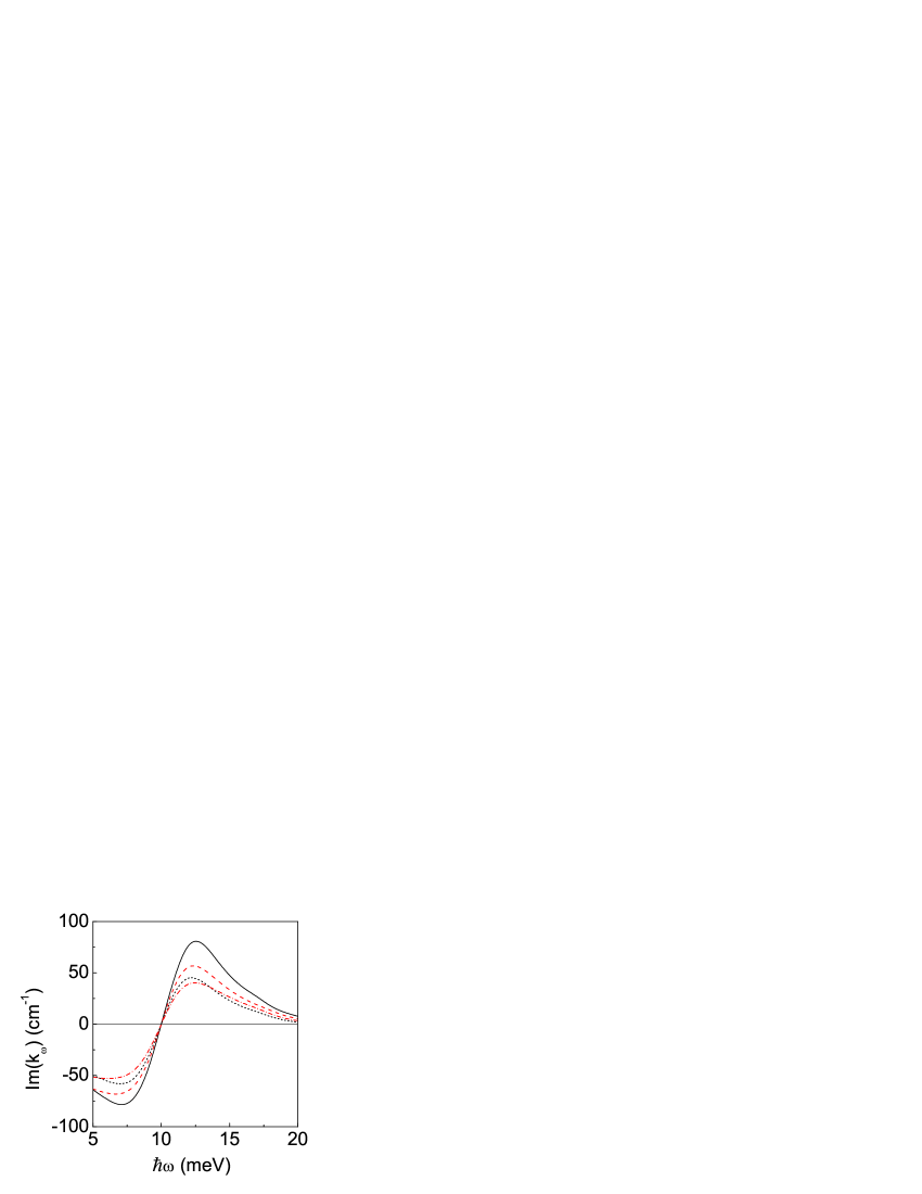
Figure 4: (Color online) Frequency dispersion of $Im(k_{\omega})$ for a metallic waveguide. Curves are marked the same as in Fig.3.

We solve the dispersion equation (20) using $\epsilon^{\scriptscriptstyle\bot,\|}$ calculated in Sec. III for the BSL width $d=4\mu$m and $L=40\mu$m. Considering the lowest mode when the real part of $k_{\omega}$ appears to be close to $\sqrt{\epsilon}\omega/c$, we have plotted $Im(k_{\omega})$ in Fig. 4 for the above cases ($\gamma=\Gamma$ and $\gamma=3\Gamma$). There are two perfectly defined spectral regions: a gain region with $Im(k_{\omega})<0$ for $\hbar\omega<\varepsilon_{\scriptscriptstyle B}$, and a damping one $Im(k_{\omega})>0$ for $\hbar\omega>\varepsilon_{\scriptscriptstyle B}$. A marked increase of the gain can be seen when temperature $T_{e}$ decreases.

IV.2 Localized Mode

For the case of a BSL placed near the vacuum-dielectric interface, we use Eqs. (15, 16) with the additional boundary conditions $E_{\scriptscriptstyle\|}(z\rightarrow\pm\infty)=0$. The wave equations for vacuum, BSL and substrate regions take the forms:

$$\left(\frac{d^{2}}{dz^{2}}-\kappa_{v}^{2}\right)E_{\scriptscriptstyle\|}(z) = 0,~{}~{}z>\frac{d}{2},$$

$$\left(\frac{d^{2}}{dz^{2}}+\kappa_{\scriptscriptstyle\bot}^{2}\right)E_{\scriptscriptstyle\|}(z) = 0,~{}~{}|z|<\frac{d}{2},$$ (21)

$$\left(\frac{d^{2}}{dz^{2}}-\kappa_{s}^{2}\right)E_{\scriptscriptstyle\|}(z) = 0,~{}~{}z<-\frac{d}{2},$$

where $\kappa_{\scriptscriptstyle\bot}$ is introduced in Sec. IIIA, $\kappa_{v}^{2}=(\omega/c)^{2}-k_{\omega}^{2}$ and $\kappa_{s}^{2}=\epsilon_{s}(\omega/c)^{2}-k_{\omega}^{2}$ with the dielectric permittivity of substrate, $\epsilon_{s}$. The field distribution is given by

$$E_{\scriptscriptstyle\|}(z)=\left\{\begin{array}[]{cc}E_{+}e^{-\kappa_{v}(z-d/2)},&z>d/2\\ e_{+}e^{i\kappa_{\scriptscriptstyle\bot}z}+e_{-}e^{-i\kappa_{\scriptscriptstyle\bot}z},&|z|<\frac{d}{2}\\ E_{-}e^{\kappa_{s}(z+d/2)},&z<-d/2\end{array}\right.,$$ (22)

where $Re(\kappa_{s,v})$ should be positive. The dispersion relation is obtained from Eqs. (21, 22) in the form:

$$\frac{\epsilon^{\scriptscriptstyle\|}}{\kappa_{\scriptscriptstyle\bot}}\left(\frac{\epsilon_{s}}{\kappa_{s}}+\frac{1}{\kappa_{v}}\right)\cos\kappa_{\scriptscriptstyle\bot}d-\left(\frac{\epsilon_{s}}{\kappa_{v}\kappa_{s}}-\frac{(\epsilon^{\scriptscriptstyle\|})^{2}}{\kappa_{\scriptscriptstyle\bot}^{2}}\right)\sin\kappa_{\scriptscriptstyle\bot}d=0.$$ (23)

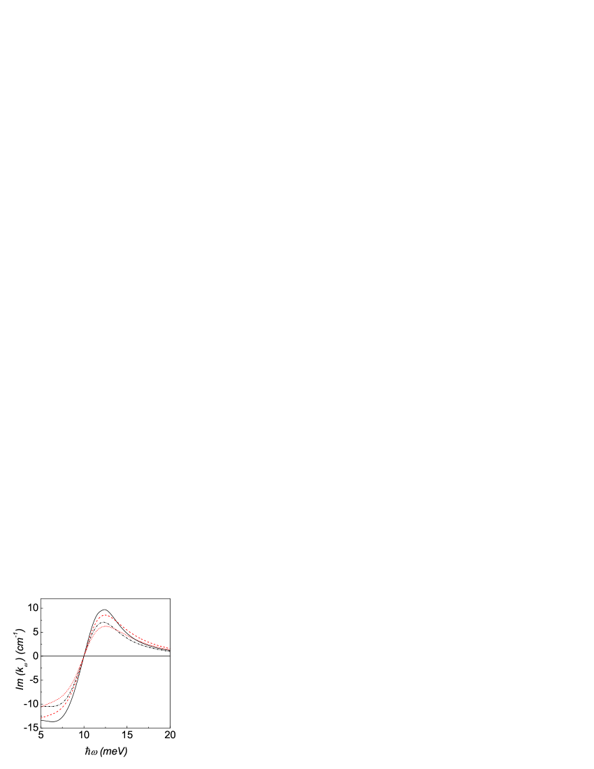
Figure 5: (Color online) Frequency dispersion of $Im(k_{\omega})$ for a dielectric waveguide. Curves are marked the same as in Fig.3.

The solution of this dispersion equation is performed for the above listed $\left(\gamma,\Gamma\right)$ and $\left(\mu,T_{e}\right)$ pairs. We use also the BSL width $d=4\mu$m and $\epsilon_{s}=3.7$, which corresponds to SiO₂ substrate. Figure 5 shows $Im(k_{\omega})$ for the cases under consideration. As in the metallic case, two regions can be selected: a gain region with $Im(k_{\omega})<0$ for $\hbar\omega<\varepsilon_{\scriptscriptstyle B}$, and a damping one where $Im(k_{\omega})>0$ for $\hbar\omega>\varepsilon_{\scriptscriptstyle B}$. Contrary to the metallic case, gain for the dielectric waveguide exists even for low energy values, at $\hbar\omega<$ 5 meV. Since $Re(\kappa_{v,s})>>Im(\kappa_{v,s})$, the transverse size of mode is determined by $Re(\kappa_{v,s})^{-1}$ which are varied from 11.3 $\mu$m at low-frequency region to $Re(\kappa_{v})^{-1}=$9.45 $\mu$m and $Re(\kappa_{s})^{-1}=$5.1 $\mu$m at $\hbar\omega=20$ meV. These results are weakly dependent on temperatures and the broadening cases under study.

V SUMMARY AND CONCLUSIONS

We have considered here the intersubband response of a biased superlattice on a THz radiation field beyond the Born approximation. Taking into account the interplay between homogeneous and inhomogeneous broadening we have analyzed the spectral and temperature dependencies of the complex dielectric permittivity in the low-doped BSL. We have found the low-frequency enhancement of the dispersion of complex dielectric permittivity and have estimated the conditions to obtain the stimulated emission regime. The enhancement of the emission due to the THz waveguide effect is also considered for the cases of the BSL placed between ideal metallic mirrors and at a vacuum-dielectric interface. The appearence of the localized THz mode due to BSL placed at the interface vacuum-dielectric is described.

Let us briefly discuss the assumptions used in the present calculations. The main restriction of the results is the description of the response in the framework of the tight-binding approach (within an accuracy of the order $T^{2}$) which is valid under the condition $\varepsilon_{\scriptscriptstyle B}>2T$ and is satisfied for the numerical estimates performed. Note that beyond the Born approximation the broadening can be comparable to the averaged electron energy. Next, in spite of the general equations (10) and (14) are written through an arbitrary spectral density function, with the use of statistically independent random potentials in each QW, final calculations were performed for a model that includes scattering by zero-radius centers and large-scale potential. Such a model describes the interplay between homogeneous and inhomogeneous mechanisms of broadening . Other approximations we have made are rather standard. We restrict ourselves to the case of uniform biased field and QW population neglecting a possible domain formation caused by the negative differential conductivity of BSL 3 ; 19 . One can avoid instabilities in a short enough BSL because the THz modes propagate in the in-plane directions. The Coulomb correlations, which modify the response as the concentration increases, are not taken into account here. This contribution, as well as the consideration of an intermediate-scale potential, requires a special attention in analogy with the case of a single QW 20 . Finally, the simplified description of the ideal (without any damping) waveguide structure is enough to estimate the characteristic planar size of a device suitable for THz stimulated emission: one have to compare the maximal negative value of $Im(k_{\omega})$ obtained with a damping length calculated for similar waveguides, see 21 . Note, that more complicate waveguides (see Refs. in 22 ) may be effective

To conclude, the simplifications listed do not change the peculiarities of the THz response or the numerical estimates given in Sec. IV. It seems likely that the contribution of $Re(\Delta\epsilon_{\omega})$ can be found experimentally. More detailed numerical simulations are necessary in order to estimate a potential for applications of BSL as a THz emitter.

References

(1) C. Gmachl, F. Capasso, D.L. Sivco, and A.Y. Cho, Reports on
Progr. in Phys. 64, 1533 (2001); J. Faist, D. Hofstetter, M. Beck,
T. Aellen, M. Rochat, and S. Blaser, IEEE J. of Quant. Electr. 38,
533 (2002).
(2) A. Tredicucci, R. Kohler, L. Mahler, H.E. Beere, E.H. Linfield,
and D.A. Ritchie, Semicond. Sci. Technol. 20, S222 (2005).
(3) L.L. Bonilla and H.T. Grahn, Reports on Prog. in Phys. 68, 577 (2005).
(4) A. Wacker, Phys. Rep. 357, 86 (2002).
(5) S.A. Ktitorov, G.S. Simin, and V.Ya Sindalovskii, Sov. Phys.
Solid State, 13 1872 (1971); A.A. Ignatov and Yu.A. Romanov, Phys.
Status Solidi B, 73 327 (1976); A.A. Ignatov, E.P. Dodin, and V.I.
Shashkin, Mod. Phys. Lett. B5, 1087 (1991); A.A. Ignatov, K. F.
Renk, and E.P. Dodin, Phys. Rev. Lett. 70, 1996 (1993).
(6) N. V. Demarina and K. F. Renk, Phys. Rev. B 71, 035341 (2005);
V.N. Sokolov, L. Zhou, G.J. Iafrate, and J.B. Krieger, Phys. Rev. B 73,
205304 (2006).
(7) Y. Shimada, K. Hirakawa, M. Odnoblioudov, and K. A. Chao, Phys.
Rev. Lett. 90 046806 (2003); Y. Shimada, N. Sekine, and K.
Hirakawa, Appl. Phys. Lett. 84, 4926 (2004);
(8) N. Sekine and K. Hirakawa, Phys. Rev. Lett. 94 057408
(2005); K. Hirakawa and N. Sekine, Physica E 32, 320 (2006).
(9) P.G. Savvidis, B. Kolasa, G. Lee, and S.J. Allen, Phys. Rev.
Lett. 92 196802 (2004); P. Robrisha, J. Xub, S. Kobayashic, P.G.
Savvidis, B. Kolasa, G. Lee, D. Mars, and S.J. Allen, Physica E 32,
325 (2006).
(10) H. Willenberg, G. H. Dohler, and J. Faist, Phys. Rev. B 67 085315 (2003).
(11) F.T. Vasko, Phys. Rev. B 69, 205309 (2004).
(12) F.T. Vasko and A.V. Kuznetsov, Electron States and
Optical Transitions in Semiconductor Heterostructures (Springer, New York,
1998).
(13) F.T. Vasko and O.E. Raichev, Quantum Kinetic Theory and
Applications (Springer, New York, 2005).
(14) Such transformations of Eq. (7) give us
(15) Transformation from Eq.(8) to (9) is performed with the use:
(17) T. Ando, A.B. Fowler, F. Stern, Rev. Mod. Phys. 54,
437 (1982).
(18) For the Gaussian case, , the convolution of spectral
densities takes the form: . Similar behavior, with a more complicate analytical function,
takes place for the Lorentzian case.
(19) D.A. Dahl and L.J. Sham, Phys. Rev. B 16, 651 (1977).
(20) E. Scholl, Nonequilibrium Phase Transitions in
Semiconductors (Springer, Berlin, 1987).
(21) F.T. Vasko, P. Aceituno, and A. Hernández-Cabrera, Phys.
Rev. B 66 125303 (2002); F.T. Vasko, JETP 93 1270, (2001).
(22) S. Kohen, B.S. Williams, and Qing Hu, J. of Appl. Phys. 97, 053106 (2005).
(23) W. Zietkowski and M. Zaluzny, J. of Appl. Phys. 96,
6029 (2004).