Quantum dynamics of repulsively bound atom pairs in the Bose-Hubbard model

Abstract

We investigate the quantum dynamics of repulsively bound atom pairs in an optical lattice described by the periodic Bose-Hubbard model both analytically and numerically. In the strongly repulsive limit, we analytically study the dynamical problem by the perturbation method with the hopping terms treated as a perturbation. For a finite-size system, we numerically solve the dynamic problem in the whole regime of interaction by the exact diagonalization method. Our results show that the initially prepared atom pairs are dynamically stable and the dissociation of atom pairs is greatly suppressed when the strength of the on-site interaction is much greater than the tunneling amplitude, i.e., the strongly repulsive interaction induces a self-localization phenomenon of the atom pairs.

I Introduction

The ultracold bosonic atoms in optical lattices have opened a new window to study many-particle quantum physics in a uniquely controlled manner Bloch ; Greiner ; Stoeferle . Various schemes have been proposed to realize a wide range of many-body Hamiltonians by loading ultracold atoms into a certain optical lattice Jaksch2005 ; Jaksch ; Duan . The advances in the manipulation of atom-atom interactions by Feshbach resonances Inouye allowed experimental study of many-body systems accessible to the full regime of interactions, even to the very strongly interacting Tonks-gas limit Kinoshita ; Tonks . Recently a lot of exciting experiments in optical lattices have been implemented, including the superfluid-Mott-insulator transition Greiner ; Stoeferle , non-linear self-trapping in a periodical optical lattice Anker and repulsively bound atom pairs in an optical lattice Winkler . The basic physics of the ultracold atomic systems in optical lattice is captured by the Bose-Hubbard model (BHM) Jaksch ; Jaksch2005 , which incorporates the competition between the interaction and hopping energy and has been successfully applied to interpret the superfluid-Mott-insulator transition. As a fundamental model, the BHM has been widely applied to study the quantum phase transitions and dynamic problems in the optical lattices.

Very recently, Winkler et al. Winkler have studied the dynamical evolution of the initially prepared bosonic atom pairs in an optical lattice. Their experimental results indicate that the atom pairs with strongly repulsive on-site interaction $U$ exhibits a remarkably longer lifetime than the system with weakly repulsive interaction Winkler . At first glance, this result is counter-intuition because one may expect the repulsive interaction to separate the particles, instead to bind them together. The experimental result has stimulated theoretical investigations on the dynamics of repulsively bound pairs Denschlag ; Petrosyan . In Ref.Winkler , the theoretical understanding of the stable pair relies on the analytical solution of a two-particle problem by solving two particle Lippmann-Schwinger scattering equation on the lattice corresponding to the Bose-Hubbard HamiltonianWinkler ; Denschlag . Obviously, this method is only limited to a single repulsively bound pair and is not capable to extend to deal with many-particle dynamic problem.

Motivated by the experimental progress Winkler , in this paper we study the quantum dynamics of the repulsively pair states in the BHM both analytically and numerically. In the strongly repulsive limit, we develop an analytical method to deal with the dynamical problem based on the perturbation expansion of the hopping terms, whereas we can numerically solve the dynamic problem in the whole regime of interaction for a finite-size system which could be diagonalized exactly by the exact diagonalization method. The Bose-Hubbard Hamiltonian (BHH) reads Jaksch ; Fisher

$$\hat{H}=-J\sum_{\left\langle i,j\right\rangle}\hat{b}_{i}^{\dagger}\hat{b}_{j}+\frac{1}{2}U\sum_{i}\hat{n}_{i}(\hat{n}_{i}-1),$$ (1)

where $\hat{b}_{i}^{\dagger}(\hat{b}_{j})$ is the creation (annihilation) operator of bosons on site $i$ $(j)$, $\hat{n}_{i}=\hat{b}_{i}^{\dagger}\hat{b}_{i}$ counts the number of bosons on the $i$th site, and $\left\langle i,j\right\rangle$ denotes summation over nearest neighbors. The parameter $J$ denotes the hopping matrix element to neighboring sites, and $U\propto a_{s}$ represents the on-site interaction due to s-wave scattering. For an actual optical lattice, $J$ and $U$ are related to the depth of the optical lattice $V_{0}$ which is determined by the intensity of the laser. The lattice constant $a$ is half of the wave length of the laser $\lambda/2$ Jaksch . In this article, we focus on the dynamical evolution of the repulsively bound atom pairs in the periodic Bose-Hubbard model with $U>0$, i.e. repulsive on-site interaction. In the following calculation, we will ignore all possible dissipations in the system, such as the loss of atoms by three-body collision.

The paper is organized as follows. In Sec. II, we first review a general scheme to deal with dynamical evolution and present the exact result for the two-site problem. In Sec. III, we develop a perturbation method to study the dynamic evolution of the initially prepared state of atom pairs which works in the large $U$ limit. In Sec. IV, we study the dynamical problem for a finite-size system by using the exact diagonalization method and compare the analytical results with the exact numerical results.

II General scheme

The Bose-Hubbard model has been investigated by a variety of theoretical and numerical methods under different cases Fisher ; Stoof ; Roth ; Norman . Most of the theoretical investigations concern the ground state properties, whereas the quantum dynamic problems are hardly dealt with and most of works are limited to the double-well (two-site) problems Vardi ; Tonel .

Given an initial state $\left|\psi_{0}\right\rangle,$ the evolution state at time $t$ can be formally represented as

$$\left|\psi(t)\right\rangle=e^{-i\widehat{H}t}\left|\psi_{0}\right\rangle.$$ (2)

If we know all the eigenstates of the BHH which are the solutions of schrödinger equation $\widehat{H}\left|\phi_{n}\right\rangle=E_{n}\left|\phi_{n}\right\rangle,$ we can get

$$\left|\psi(t)\right\rangle=\sum_{n}e^{-iE_{n}t}\left|\phi_{n}\right\rangle\left\langle\phi_{n}\right.\left|\psi_{0}\right\rangle.$$ (3)

Now it is straightforward to obtain the probability of finding the given initial state at time $t$

$$P_{0}(t) = \left|\left\langle\psi(0)\right.\left|\psi(t)\right\rangle\right|^{2}$$ (4)

$$= \sum_{n=1}^{D}\sum_{m=1}^{D}\left|a_{n}\right|^{2}\left|a_{m}\right|^{2}e^{-i(E_{n}-E_{m})t},$$

where $a_{n}=\left\langle\phi_{n}\right.\left|\psi_{0}\right\rangle$ and $D=\left(N+L-1\right)!/[N!\left(L-1\right)!]$ is the basis dimension of the $N$-particle system in a lattice with size $L$. If the energy spectrum and its corresponding eigenstates $\phi_{n}$ are known, then the dynamical problem is exactly solved in principle. It is obvious that the dimension $D$ increases very quickly as the particle number $N$ and lattice site $L$ increase. Therefore it is not practical to investigate the dynamical problem of a large system in this way, though one can solve it numerically for a finite-size system by exact diagonalization method.

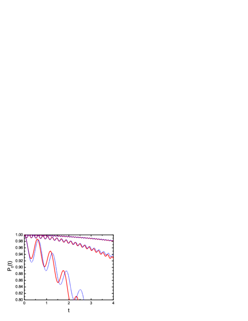
Figure 1: (Color online) Time evolution of $P_{0}(t)$ versus $t$ in units of $J$ for the two-site-two-boson case. A comparison between the exact and the approximate solution is made. The solid lines denote the exact solutions given in Sec. II. The dotted lines denote the approximate solutions by perturbation theory. From top to bottom the lines correspond to $U/J=60$, $30$ and $10$, respectively.

It is instructive to study the two-site system before presenting the analytical results based on perturbation theory and the numerical results for the systems with larger size. The dynamical evolution of an atom pair in the toy two-site model can be completely solved analytically. The results of this toy model will shed light on studies of larger systems. According to the scheme discussed above, it is quite easy to get the analytical expression of $P_{0}(t)$ for a pair of atoms initially in a two-site lattice:

$$P_{0}(t) = \left|a_{1}\right|^{4}+\left|a_{2}\right|^{4}+\left|a_{3}\right|^{4}$$ (5)

$$+2\left|a_{1}\right|^{2}\left|a_{2}\right|^{2}\cos\left(E_{1}-E_{2}\right)t$$

$$+2\left|a_{2}\right|^{2}\left|a_{3}\right|^{2}\cos\left(E_{2}-E_{3}\right)t$$

$$+2\left|a_{3}\right|^{2}\left|a_{1}\right|^{2}\cos\left(E_{3}-E_{1}\right)t,$$

where $a_{1}=1/\sqrt{2}$, $a_{2}=1/\sqrt{2+\alpha^{2}}$ and $a_{3}=1/\sqrt{2+\beta^{2}}$ with the parameters $\alpha=-4\sqrt{2}J/\left(U-\sqrt{U^{2}+16J^{2}}\right)$ and $\beta=-4\sqrt{2}J/\left(U+\sqrt{U^{2}+16J^{2}}\right)$. The eigenenergies are given by $E_{1}=U$, $E_{2}=\left(U-\sqrt{U^{2}+16J^{2}}\right)/2$, and $E_{3}=\left(U+\sqrt{U^{2}+16J^{2}}\right)/2$. It is quite easy to show the time evolution of the initial atom pair by the formula (5). In Fig. 1, we plot the time evolution of $P_{0}(t)$ for $U/J=60$, $30$ and $10$. The results show that the larger the repulsive $U$ is, the probability of finding the initial atom pair is larger. When $U/J\rightarrow\infty$, we observe that $a_{2}\rightarrow 0$, $a_{3}\rightarrow 1/\sqrt{2}$, $E_{1}-E_{2}\approx E_{3}-E_{2}\approx U$ and $E_{3}-E_{1}\approx 4J^{2}/U$. In this limit, the terms including of $a_{2}$ in Eq. (5), which is proportional to $\frac{J}{U}\cos(Ut)$, merely give a very tiny contribution to $P_{0}(t)$ accompanying with a very high-frequency oscillation, whereas the dominant part is given by

$$P_{0}(t)\approx\frac{1}{2}+\frac{1}{2}\cos(4\frac{J^{2}}{U}t).$$ (6)

It is obvious that $P_{0}(t)\approx 1$ if $Jt\ll U/J$. Therefore at the large $U$ limit, the atom pair is dynamically stable within a very large time scale.

III Dynamics in the large U limit

In the strongly repulsive interaction limit of $U/J\gg 1$, it is convenient to represent the BHH as

$$\widehat{H}=\widehat{H}_{U}+\widehat{H}_{J},$$

where $\widehat{H}_{U}$ and $\widehat{H}_{J}$ are the on-site interaction part and tunnelling part respectively. We may solve the following dynamical evolution equation

$$\left|\psi(t)\right\rangle=e^{-i\widehat{H}_{J}t-i\widehat{H}_{U}t}\left|\psi_{0}\right\rangle$$ (7)

approximately by treating $\widehat{H}_{J}$ as a perturbation. In order to do that, we formally represent $\left|\psi(t)\right\rangle$ as

$$\left|\psi(t)\right\rangle=e^{-i\widehat{H}_{U}t}U(t)\left|\psi_{0}\right\rangle$$ (8)

with $U(t)$ defined as $U(t)=e^{i\widehat{H}_{U}t}e^{-i\widehat{H}_{J}t-i\widehat{H}_{U}t}$. It is easy to check that $U(t)$ fulfills the following motion of equation

$$\frac{\partial}{\partial t}U(t)=-i\widehat{H}_{J}(t)U(t)$$

with

$$\widehat{H}_{J}(t)=e^{i\widehat{H}_{U}t}\widehat{H}_{J}e^{-i\widehat{H}_{U}t}.$$

Therefore the formal solution of $U(t)$ is given by

$$U(t) = T\exp\left[-i\int_{0}^{t}dt_{1}\widehat{H}_{J}(t_{1})\right]$$

$$= \sum_{n=0}^{\infty}\frac{\left(-i\right)^{n}}{n!}\int_{0}^{t}dt_{1}\cdots\int_{0}^{t}dt_{n}T\left[\widehat{H}_{J}(t_{1})\cdots\widehat{H}_{J}(t_{n})\right],$$

where $T$ is the time-ordering operator. By using the above formula, now we can calculate $\left\langle\psi(0)\right.\left|\psi(t)\right\rangle$ perturbatively. Up to the second order, we get

$$\left\langle\psi(0)\right.\left|\psi(t)\right\rangle$$ (9)

$$= \left\langle\psi_{0}\right|e^{-i\widehat{H}_{U}t}\left|\psi_{0}\right\rangle-$$

$$\left\langle\psi_{0}\right|e^{-i\widehat{H}_{U}t}\int_{0}^{t}dt_{1}\int_{0}^{t_{1}}dt_{2}\widehat{H}_{J}(t_{1})\widehat{H}_{J}(t_{2})\left|\psi_{0}\right\rangle.$$

From the definition of $\left|\psi(t)\right\rangle,$ we see that it should be normalized. However, in the scheme of perturbation calculation, the normalized condition is not automatically fulfilled. In order to overcome this problem and get a well-defined $P_{0}(t)$, we need use a normalized $\left|\widetilde{\psi}(t)\right\rangle$ which is defined as

$$\left|\widetilde{\psi}(t)\right\rangle=\frac{\left|\psi(t)\right\rangle}{\sqrt{\left\langle\psi(t)\right.\left|\psi(t)\right\rangle}}.$$ (10)

Therefore in the scheme of perturbation expansion, the probability $P_{0}(t)$ is defined by

$$P_{0}(t)=\left|\left\langle\psi(0)\right.\left|\widetilde{\psi}(t)\right\rangle\right|^{2}.$$ (11)

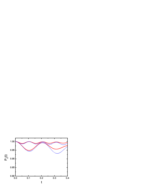
Figure 2: (Color online) Time evolution of $P_{0}(t)$ for the six-site-six-boson case. The comparison between the solution given by perturbation theory and the exact solution from numerical computation is shown. The analytical results are denoted by the dotted lines and the numerical result by solid lines. The top two lines correspond to $U/J=60$ and the other two lines correspond to $U/J=30$. The time is in units of $J$.

For a given initial state $\left|\psi_{0}\right\rangle$ represented in a basis of Fock states

$$\left|\psi_{0}\right\rangle=\left|n_{1},n_{2},...,n_{i},...,n_{L}\right\rangle$$ (12)

with $n_{i}=0$ or $2,$ it is easy to get $\widehat{H}_{U}$ $\left|\psi_{0}\right\rangle=\frac{N}{2}U$ $\left|\psi_{0}\right\rangle.$ For convenience, we first calculate the case with $\left|\psi_{0}\right\rangle=\left|2,0,2,0...,2,0\right\rangle$. By using the formula (9), we get

$$\left\langle\psi(0)\right.\left|\psi(t)\right\rangle$$ (13)

$$= e^{-i\frac{N}{2}Ut}\left[1-i\frac{2NJ^{2}t}{U}+\frac{2NJ^{2}}{U^{2}}\left(e^{iUt}-1\right)\right].$$

Therefore we have

$$P_{0}(t) = A^{-1}\left[1-\left(\frac{4NJ^{2}}{U^{2}}-\frac{8N^{2}J^{4}}{U^{4}}\right)\left(1-\cos Ut\right)+\right.$$ (14)

$$\left.\frac{4N^{2}J^{4}t^{2}}{U^{2}}-\frac{8N^{2}J^{4}t}{U^{3}}\sin Ut\right]$$

where $A=\left\langle\psi(t)\right.\left|\psi(t)\right\rangle$ is the normalized constant. We note that, in the scheme of the second-order perturbation theory, formula (13) has the same form for different initial configurations such as $\left|\psi_{0}\right\rangle=\left|2,0,2,0,0,2,0,0,0\right\rangle$ and $\left|\psi_{0}\right\rangle=\left|2,0,2,0,2,0,0,0,0\right\rangle$. Actually, the formula (13) is valid for all the initial configurations where the atoms pairs are not neighboring to each others. For the other kind of initial configurations, it is straightforward to calculate $P_{0}(t)$ by formula (11) and (9).

In order to check the validity of the perturbation theory, we plot the $P_{0}(t)$ obtained by the perturbation theory for the two-site problem in Fig. 1 and make a rough comparison between the perturbation result and the exact result given in Eq. (5). Specially, for the simplest two-site case with $\left|\psi_{0}\right\rangle=\left|2,0\right\rangle$ or $\left|0,2\right\rangle$, we have

$$P_{0}(t) = {A}^{-1}\left[1-\left(\frac{4J^{2}}{U^{2}}-\frac{8J^{4}}{U^{4}}\right)\left(1-\cos Ut\right)+\frac{4J^{4}t^{2}}{U^{2}}-\right.$$ (15)

$$\left.\frac{8J^{4}t}{U^{3}}\sin Ut\right],$$

where the normalization constant $A$ is given by

$$A=1+8J^{4}\left[\frac{2}{U^{4}}\left(1-\cos Ut\right)-\frac{2t}{U^{3}}\sin Ut+\frac{t^{2}}{U^{2}}\right].$$ (16)

As is shown in Fig. 1, the larger the $U$, the better the exact and the approximate solution fit.

It is natural to use the formula (11) to deal with the many-particle system. From (13), we see that the perturbation theory should work well as long as $NJ^{2}t/U\ll 1$. In order to compare with the exact result by numerical exact diagonalization method in next section, we apply (14) to calculate the time evolution of $P_{0}(t)$ for a finite-size system with an initial state $\left|\psi_{0}\right\rangle=\left|2,0,2,0,2,0\right\rangle.$ Our result is shown in Fig. 2. We can see that at large $U$ limit, the perturbation theory works quite well. Our results show that $\psi(t)$ decays slower for a larger $U$. For a larger system with $N=50$ and the initial state given by $\left|2,0,2,0,...,2,0,2,0\right\rangle$, the time evolution of $P_{0}(t)$ shows similar behaviors as that of the 2- and 6-particle systems. As shown in Fig. 3, $P_{0}(t)$ decays slowly accompanying with a high-frequency but very narrow oscillation. These results show that, when $U$ is large enough, $\psi(t)$ mainly stays in the initial state within a large time scale. The larger the U is, the more obvious the case.

Figure 3: Time evolution of $P_{0}(t)$ for the 50-particle system with initial state $\left|2,0,2,0,...,2,0,2,0\right\rangle$ versus $t$ in units of $J$ with the corresponding on-site interaction $U/J=200$.

IV Numerical result

The exact diagonalization (ED) method is very powerful from the viewpoint that it can give out all information of the system exactly. To solve the matrix eigenvalue problem of the Hamiltonian, it is convenient to work in a basis of Fock states

$$\left|\alpha\right\rangle=\left|\{n_{1},n_{2},...,n_{L}\}_{\alpha}\right\rangle,$$ (17)

with $n_{i}=0,1,2,\cdots$ and the index $\alpha=1,...,D$ labels the different compositions of occupation numbers for a fixed total particle number $\sum_{i=1}^{L}n_{i}=N$. Through the exact diagonalization algorithm we compute exactly all the eigenvalues $E_{n}$ and the corresponding eigenstates $\phi_{n}$ of the Hamiltonian (1). Then we can calculate the dynamic evolution of $P_{0}(t)$ by using Eq. (4). To give a concrete example and compare with the result obtained by the perturbation theory in Sec. III, we first consider an initial state $\left|\psi_{0}\right\rangle=\left|2,0,2,0,2,0\right\rangle$. Our result is shown in Fig. 2. We can see that at large $U$ limit, the perturbation theory works quite well.

We note that what was measured in the experiment Winkler is the number of remaining pairs after a variable hold time. To understand the experimental result qualitatively, we calculate the time-dependent normalized number of the atom pairs which can be represented as

$$\bar{N}_{p}(t)=\sum_{\alpha=1}^{D}\frac{N_{p}(\alpha)\left|c_{\alpha}(t)\right|^{2}}{M},$$ (18)

where $c_{\alpha}(t)$ is given by

$$c_{\alpha}(t)=\sum_{n=1}^{D}e^{-iE_{n}t}\left\langle\alpha|\phi_{n}\right\rangle\left\langle\phi_{n}|\psi_{0}\right\rangle,$$ (19)

$N_{p}(\alpha)$ denotes the number of atom pairs in $\left|\alpha\right\rangle$ and $M=N/2$ is the total number of initial atom pairs. Using the formula (18), we can calculate the normalized atom pair number for different on-site interaction $U$ and different initial state $\left|\psi_{0}\right\rangle$.

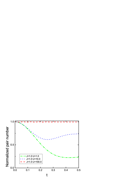
Figure 4: (Color online) Time evolution of normalized atom pair number in a nine-site optical lattice for $U/J=1.0$, $10.0$ and $100.0$. The time is in units of $J$ and the initial state is chosen as $\left|2,2,2,0,0,0,0,0,0\right\rangle$.

For simplicity, let us consider a one-dimensional (1D) optical lattice with $L=9$ and $M=3$, i.e. three boson atom pairs loaded into an optical lattice of nine sites. The time dependent normalized pair numbers for various interaction strengths are plotted in Fig. 4 with the initial state given by $\left|2,2,2,0,0,0,0,0,0\right\rangle$. Evidently, the atom pairs in the case of $U=100.0$ stay longer than that in the case of $U=1.0$. It is clear that the large on-site interaction $U$ effectively suppresses the dynamic dissociation of the initial pairs, which is in qualitative agreement with the experiment reported in Ref. Winkler .

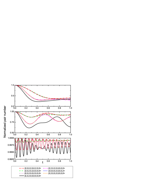
Figure 5: (Color online) Time evolution of the normalized atom pair number for different on-site interaction $U$ and different initial states $\left|\psi_{0}\right\rangle$. From top to bottom the on-site interaction $U/J$= 1.0, 10.0, and 100.0, respectively. In each graph, there are seven lines corresponding to seven different initial states. The initial states are denoted by different lines shown in the table at the bottom. The time is in units of $J$.

Next we study how the dynamics of the repulsively bound pairs is affected by the choice of the initial state. For the case with three bound pairs loaded into an optical lattice with nine sites, there are $C_{9}^{3}=84$ different configurations. Taken the translational symmetry of the system into account, there are in fact only seven different configurations. For different initial state $\left|\psi_{0}\right\rangle$, we calculate the normalized atom pair number and plot them in Fig. 5. According to Fig. 5, although for different initial state $\left|\psi_{0}\right\rangle$ the corresponding dynamics of the system is similar to each other, there are still some minor differences depending on whether the initial pairs are close together or not. For initial states $\left|2,0,2,0,2,0,0,0,0\right\rangle$, $\left|2,0,2,0,0,2,0,0,0\right\rangle$, and $\left|2,0,0,2,0,0,2,0,0\right\rangle$ in which each pair is apart from the others, the time evolutions are almost the same. This is consistent with our result by perturbation theory. According to the second-order perturbation theory, the time evolution of $P_{0}(t)$ for these initial states are same. Similarly, the time evolution for initial states $\left|2,2,0,2,0,0,0,0,0\right\rangle$, $\left|2,2,0,0,2,0,0,0,0\right\rangle$, and $\left|2,2,0,0,0,2,0,0,0\right\rangle$ are almost the same for different on-site interaction $U$ as is shown in Fig. 5. We notice that the initial states with bound pairs repelling each other are dynamically stabler than the states with all atom pairs initially occupying neighboring sites. We also investigate the case in which there are three boson atom pairs loaded into a two-dimensional $3\times 3$ optical lattice. The results are similar to the one-dimensional case as shown in Fig. 4 and Fig. 5.

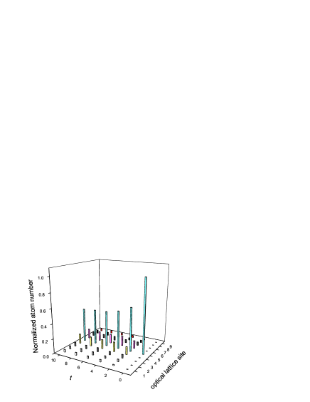
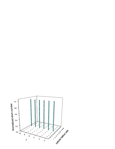
Figure 6: Time evolution of the normalized atom number on each site of the optical lattice. We choose the initial state $\left|\psi_{0}\right\rangle$ as $\left|0,0,0,0,6,0,0,0,0\right\rangle$. The graph on the top corresponds to $U/J$=1.0 and the graph on the bottom to $U/J$=10.0. The time is in units of $J$.

From above discussions, we could understand the stable atom-pair state due to the strongly repulsive interaction as a dynamically stable state. The physical origin is essentially that the energy conservation does not allow the particle to tunnel into the neighboring sites to save the repulsive interaction unless the obtained tunneling energy is comparable to the loss of repulsive energy BlochRMP . From theoretical point of view, a similar dynamically stable state is expected to appear for the case in which the initial state composed of three or more atoms. In order to clarify this point, we investigate an example case in which six atoms were initially loaded into only one site of a 1D optical lattice with nine sites. The initial state is chosen as $\left|0,0,0,0,6,0,0,0,0\right\rangle$. Given the initial state, we then determine the dynamic evolution of the initial state on the whole lattice, i.e., the spatial distribution of the normalized atom number on each site at different time point for different on-site interaction. The time-dependent normalized atom number on the $j$-th site can be calculated by

$$\bar{n}_{j}(t)=\sum_{\alpha=1}^{D}\frac{\left|c_{\alpha}(t)\right|^{2}n_{j}^{\alpha}}{N},$$ (20)

where $n_{j}^{\alpha}=\left\langle\alpha\right|\hat{n}_{j}\left|\alpha\right\rangle$. The spatial distributions provide us useful information for the expansion dynamics of a condensate loaded in the optical lattice. At an incremental sequence of time points, we calculate the normalized atom number at each site. The results are shown in Fig. 6. For a small $U$ $(U=J)$, the atoms initially trapped in a site tend to tunnel to the neighboring sites and thus lead to the decrease of the normalized atom number in the initial site. However, when the on-site $U$ is large enough, the initially trapped atoms are dynamically frozen and the expansion to the neighboring sites is almost completely suppressed.

V summary

In this paper, we theoretically investigate the dynamical stability of atom pairs induced by the strongly repulsive interaction in an optical lattice both analytically and numerically. Firstly, in the large $U$ limit, we calculate the time evolution of an initial system composed of atom pairs in a scheme of the perturbation theory. The analytical results show that the initial state of atom pairs is dynamically stabler for larger repulsive interaction. Then by the exact diagonaliztion method, we numerically study the stability of atom pairs in a finite-size system with few particles by calculating the time evolution of the normalized atom pair number. Our results show that the initial state of atom pairs are dynamically stable and the dissociation of atom pairs is greatly suppressed when the strength of the on-site interaction is large. We also compare our numerical result with the result based on the perturbation theory and find out that they fit quite well in the large $U$ limit. Our results imply that the experimentally observed repulsively bound pairs can be understood as a dynamically stable state.

- (1) I. Bloch, Nature phys. 1, 23 (2005).
- (2) M. Greiner, O. Mandel, T. Esslinger, T. W. Hänsch, and I. Bloch, Nature (London) 415, 39 (2002).
- (3) T. Stöferle, H. Moritz, C. Schori, M. Köhl and T. Esslinger, Phys. Rev. Lett. 92, 130403 (2004).
- (4) D. Jaksch and P. Zoller, Ann. Phys. 315, 52 (2005).
- (5) D. Jaksch, C. Bruder, J. I. Cirac, C. W. Gardiner, and P. Zoller, Phys. Rev. Lett. 81, 3108 (1998).
- (6) L.-M. Duan, E. Demler, and M. D. Lukin, Phys. Rev. Lett. 91, 090402 (2003).
- (7) S. Inouye et al., Nature (London) 392, 151 (1998).
- (8) T. Kinoshita, T. Wenger and D. S. Weiss, Science 305, 1125 (2004); B. Paredes, A. Widera, V. Murg, O. Mandel, S. Fölling, I. Cirac, G. V. Shlyapnikov, T. W. Hänsch, and I. Bloch, Nature (London) 429, 277 (2004).
- (9) M. D. Girardeau, J. Math. Phys. (N.Y.) 1, 516 (1960); L. Tonks, Phys. Rev. 50, 955 (1936); V. Dunjko, V. Lorent and M. Olshanii, Phys. Rev. Lett. 86, 5413 (2001); S. Chen and R. Egger, Phys. Rev. A. 68, 063605 (2003).
- (10) T. Anker, M. Albiez, R. Gati, S. Hunsmann, B. Eiermann, A. Trombettoni, and M. K. Obethaler, Phys. Rev. Lett. 94, 020403 (2005).
- (11) K. Winkler, G. Thalhammer, F. Lang, R. Grimm, J. Hecker Denschlag, A. J. Daley, A. Kantian, H. P. Büchler, and P. Zoller, Nature (London) 441, 853 (2006).
- (12) J. Hecker Denschlag and A. J. Daley, cond-mat/0610393.
- (13) D. Petrosyan, B. Schmidt, J. R. Anglin, and M. Fleischhauer, cond-mat/0610198.
- (14) M. P. A. Fisher, P. B. Weichman, G. Grinstein, and D. S. Fisher, Phys. Rev. B. 40, 546 (1989).
- (15) D. van Oosten, P. van der Straten, and H. T. C. Stoof, Phys. Rev. A 63 053601 (2001).
- (16) R. Roth and K. Burnett, Phys. Rev. A 67, 031602 (2003).
- (17) N. Oelkers and J. Links, cond-mat/0611510.
- (18) A. Vardi and J. R. Anglin, Phys. Rev. Lett. 86, 568 (2001).
- (19) A. P. Tonel, J. Links, and A. Foerster, J. Phys. A: Math. Gen. 38, 1235 (2005).
- (20) I. Bloch, J. Dalibard, and W. Zwerger, arXiv:0704.3011.