Quantum critical point in graphene approached in the limit of infinitely strong Coulomb interaction

Abstract

Motivated by the physics of graphene, we consider a model of $N$ species of $2{+}1$ dimensional four-component massless Dirac fermions interacting through a three dimensional instantaneous Coulomb interaction. We show that in the limit of infinitely strong Coulomb interaction, the system approaches a quantum critical point, at least for sufficiently large fermion degeneracy. In this regime, the system exhibits invariance under scale transformations in which time and space scale by different factors. The elementary excitations are fermions with dispersion relation $\omega\sim p^{z}$, where the dynamic critical exponent $z$ depends on $N$. In the limit of large $N$, we find $z=1-4/(\pi^{2}N)+O(N^{-2})$. We argue that due to the numerically large Coulomb coupling, graphene (freely suspended) in vacuum stays near the scale-invariant regime in a large momentum window, before eventually flowing to the trivial fixed point at very low momentum scales.

I Introduction.

The physics of graphene, which has recently been realized in experiment Novoselov-PNAS , has currently attracted considerable interest. A graphene sheet is a two dimensional (2D) hexagonal lattice of carbon atoms, and its defining feature is the existence of two special points in the Brillouin zone around which the electron energy, according to band-structure calculations, should have a linear dependence on its momentum (“Dirac cones”), as in relativistic theories Semenoff:1984dq . Many interesting behaviors, for example, the quantum Hall effect at half-integer filling fractions, are attributed to the quasirelativistic behavior of the low energy excitations Novoselov-Nature ; Kim-Nature ; Gusynin:2005pk .

Graphene, on the other hand, differs from relativistically invariant systems in one crucial aspect. Namely, the electromagnetic interaction between fermion quasiparticles is mediated by the photon whose velocity $c$ is practically infinite compared to the fermion velocity $v\approx c/300$. The interaction therefore is an instantaneous Coulomb repulsion which breaks relativistic invariance.

As we shall see later, the importance of the Coulomb interaction is controlled by the parameter

$$\lambda=\frac{e^{2}N}{16\epsilon_{0}\hbar v}\,,$$ (1)

where $N=2$ is the spin degeneracy. It is similar to the fine structure constant, but the speed of light has been replaced by the Fermi velocity $v$. As the result, for graphene in vacuum this parameter is around 3 or 4 (it is reduced if graphene resides on a substrate with a large dielectric constant). The largeness of $\lambda$ makes unreliable any calculation based on the simple perturbation theory in the interaction strength, and seems to indicate that real graphene is hopelessly beyond quantitative theoretical control.

In this paper, we show that in the idealized limit $\lambda\to\infty$ the system becomes, in a certain sense, simple again. We shall argue that, at least for sufficiently large $N$, and perhaps even for $N=2$, $\lambda\to\infty$ is a limit where the system is tuned to quantum criticality.

Quantum critical points Sachdev play an important role in condensed matter physics. In many cases, they are described by relativistically invariant conformal field theories. The relativistic invariance of these theories is not connected to the relativity of space-time, but is a manifestation of an emergent Lorentz symmetry. In our case, the infinitely strong Coulomb interaction destroys the relativistic invariance. Instead, we shall see that the quantum critical point $\lambda=\infty$ is characterized by a nontrivial dynamic critical exponent $z$, whose value is computable in the large-$N$ limit,

$$z=1-\frac{4}{\pi^{2}N}+O(N^{-2}).$$ (2)

The elementary excitations are fermions with dispersion relation $\omega\sim p^{z}$, instead of the linear dispersion $\omega=vp$. The Dirac cones are therefore replaced by “Dirac cusps.” Moreover, the full dynamics is invariant under the scale transformation

$$t\to l^{z}t,\qquad\bm{x}\to lx$$ (3)

instead of the usual “relativistic” scale transformation

$$t\to lt,\qquad\bm{x}\to lx.$$ (4)

The limit $\lambda\to\infty$ can therefore be considered as a nice idealization of graphene. While it is only an idealization, we think that its simplicity justifies our study. Moreover, one may hope that once the limit $\lambda\to\infty$ is understood, the case of finite but large $\lambda$ can be accommodated by treating $\lambda^{-1}$ as a small coefficient of a relevant deformation that takes the system away from the critical point.

The structure of this paper is as follows. In Sec. II, we describe our model. We write down the renormalization group (RG) equation in Sec. III and discuss the strong-coupling fixed point where the scaling behavior (3) is realized. The running of the fermion velocity at finite Coulomb coupling is considered in Sec. IV. In Sec. V, we discuss finite $N$ and the relevance of our model to real graphene. We conclude in Sec. VI. While a large fraction of technical calculations presented in this paper are not new, we believe that the strong-coupling limit has not been previously identified as a quantum critical point.

II Model

We shall consider a system of $N$ (2+1) dimensional [(2+1)D] four-component massless Dirac fermions with velocity $v$ interacting through an instantaneous three dimensional (3D) Coulomb interaction. The Euclidean action is (in this paper, we set $\hbar=1$)

$$S=-\sum_{a=1}^{N}\int\!dt\,d^{2}x\,(\bar{\psi}_{a}\gamma^{0}\partial_{0}\psi_{a}+v\bar{\psi}_{a}\gamma^{i}\partial_{i}\psi_{a}+iA_{0}\bar{\psi}_{a}\gamma^{0}\psi_{a})+\frac{1}{2g^{2}}\int\!dt\,d^{3}x\,(\partial_{i}A_{0})^{2}.$$ (5)

Our notations are as follows. The fields $\psi_{a}$ are four-component fermion fields, and $a$ labels different species of fermions. In real graphene $N$, is equal to 2 due to the spin degeneracy. The $\gamma$’s are (2+1)D Dirac matrices satisfying $\{\gamma^{\mu},\gamma^{\nu}\}=2\delta^{\mu\nu}$, and can be chosen as $4\times 4$ matrices, e.g., $\gamma^{0}=\sigma^{3}\otimes\sigma^{3}$, $\gamma^{i}=\sigma^{i}\otimes\openone$. Each fermion can be thought of as a pair of two-component fermions with opposite parities Nielsen:1980rz ; Nielsen:1981xu . $A_{0}$ is the Coulomb potential. The action (5) contains a (2+1)D part, which contains the kinetic term for the fermion and the interaction between the fermion and the Coulomb potential, and a (3+1) dimensional part, which is the kinetic term for the Coulomb potential. A more general model was considered in Ref. YeSachdev in the context of the quantum Hall effect. If graphene is in vacuum (as it is the case for freely suspended graphene sheets suspended ), then $g^{2}=e^{2}/\epsilon_{0}$, where $e$ is the electron charge and $\epsilon_{0}$ is the vacuum permeability. In the presence of a substrate with a dielectric constant $\varepsilon$, the effective charge is reduced,

$$g^{2}=\frac{2}{1+\varepsilon}\frac{e^{2}}{\epsilon_{0}}\,.$$ (6)

In Eq. (5), we have not included any contact four-Fermi interactions, which are irrelevant at weak coupling. At strong coupling, however, these interactions develop nontrivial fixed points Herbut:2006cs . We shall assume that these four-Fermi interactions start out with small couplings and flow to the trivial fixed point.

We will be particularly interested in the limit of infinite Coulomb repulsion $g^{2}\to\infty$. In this limit, there is no kinetic term for $A_{0}$ in the bare action (5); however, an effective kinetic term will be generated by the fermion loop. We find it useful to keep $g^{2}$ large but finite for the purpose of regularization and for the discussion of the real graphene.

Without the coupling to the scalar potential $A_{0}$, the theory is that of free Dirac fermions which is invariant under the relativistic scale transformation (4). Our goal is to see that after coupling to the scalar potential the system remains scale invariant, but under a more general type of scale transformation with a (generally) fractional $z$.

A relativistic counterpart of our model was considered previously. In Refs. Templeton:1981ei ; Templeton:1981yp free fermions are coupled to a gauge field $A_{\mu}$. At sufficiently large $N$, the infrared limit of the new system is described by a conformal field theory. (For $N$ smaller than some critical value, which is still not exactly known, it was argued that the system develops a mass gap Appelquist:1988sr .) The difference between our case and the case considered in Refs. Templeton:1981ei ; Templeton:1981yp is the lack of Lorentz invariance due to the instantaneous Coulomb interaction. The fact that in graphene Coulomb interaction induces a logarithmic renormalization of the fermion velocity and leads to logarithmic corrections in thermodynamics is well known Gonzalez:1993uz . To make the paper self-contained, we repeat some of the calculations in the literature. To start, let us state the Feynman rules that follow from Eq. (5),

• The fermion propagator is

  $$G_{0}(p)=\frac{i}{{p\hskip-7.0pt\diagup}}=\frac{i{p\hskip-7.0pt\diagup}}{p^{2}}\,.$$ (7)

  Here we use quasirelativistic notation, where $p$ stays for $(p_{0},{\vec{p}})$ (for example $d^{3}p\equiv dp_{0}\,d{\vec{p}}$) and ${p\hskip-7.0pt\diagup}\equiv\gamma^{0}{\vec{p}}_{0}+v{\vec{\gamma}}\cdot{\vec{p}}$, $p^{2}\equiv p_{0}^{2}+v^{2}|{\vec{p}}|^{2}$, and ${\vec{p}}$ is the 2D momentum vector.

• The $A_{0}$ propagator is the integral of the 3D propagator $g^{2}/(p_{z}^{2}+|{\vec{p}}|^{2})$ over the momentum component perpendicular to the 2D plane, $p_{z}$,

  $$D_{0}(p)=g^{2}\int\!\frac{dp_{z}}{2\pi}\,\frac{1}{p_{z}^{2}+|{\vec{p}}|^{2}}=\frac{g^{2}}{2|{\vec{p}}|}\,.$$ (8)

  and is simply the 2D Fourier transform of the function $g^{2}/(4\pi r)$.

• The interaction vertex is $i\gamma^{0}$.

For the simplicity of the notations, one can perform calculations using the unit system where $v=1$, then restore $v$ at the end results by dimensionality. To have analytic control, we shall work in the large-$N$ limit and then extrapolate to $N=2$. Each fermion loop comes with a factor of $N$, so in the large-$N$ limit one has to resum the fermion loop in the photon propagator (this is identical to the random phase approximation). The fermion loop is naively divergent; however, in any gauge-invariant regularization scheme (e.g., dimensional regularization) it is convergent. The resummed Coulomb propagator is (see the Appendix)

$$D(q)=\left(\frac{2|{\vec{q}}|}{g^{2}}+\frac{N}{8}\frac{|{\vec{q}}|^{2}}{\sqrt{q^{2}}}\right)^{-1}.$$ (9)

Since $D(q)\sim 1/N$, even in the $g^{2}\to\infty$ limit the interaction between fermions remains weak at large $N$, enabling a perturbative calculation.

III Renormalization group and the strong-coupling fixed point

We shall now perform Wilson RG in our theory at the leading nontrivial order in $1/N$. We assume that the theory has a cutoff $\Lambda_{0}$, and proceed to integrate out all momenta between $\Lambda_{1}$ and $\Lambda_{0}$, where $\Lambda_{1}$ is smaller than $\Lambda_{0}$ by an exponential factor. The leading $1/N$ correction to the fermion kinetic term comes from the one-loop fermion self-energy graph,

$$\Sigma(p)=-g^{2}\int\!\frac{d^{3}q}{(2\pi)^{3}}\,\frac{\gamma^{0}({p\hskip-7.0pt\diagup}-{q\hskip-7.0pt\diagup})\gamma^{0}}{(p-q)^{2}}\,\left(2|{\vec{q}}|+\frac{g^{2}N}{8}\frac{|{\vec{q}}|^{2}}{\sqrt{q^{2}}}\right)^{-1},$$ (10)

where integration is over $q$ in the momentum shell $\Lambda_{1}<q<\Lambda_{0}$. In RG, we are interested only in the contribution proportional to $\ln(\Lambda_{0}/\Lambda_{1})$.

Although the integral can be computed in closed analytic form for any $\lambda$ (see below), it is instructive to consider first the limit $\lambda=\infty$. In this limit, we find

$$\Sigma(p)=\Sigma_{0}\gamma_{0}p_{0}+\Sigma_{1}{\vec{\gamma}}\cdot{\vec{p}},$$ (11)

where $\Sigma_{0}$ and $\Sigma_{1}$ are represented as integrals,

$$\Sigma_{0}=\frac{8}{N}\int\!\frac{d^{3}q}{(2\pi)^{3}}\,\frac{q_{0}^{2}-{\vec{q}}^{2}}{(q^{2})^{3/2}|{\vec{q}}^{2}|}\,,\qquad\Sigma_{1}=\frac{8}{N}\int\!\frac{d^{3}q}{(2\pi)^{3}}\,\frac{q_{0}^{2}}{(q^{2})^{3/2}|{\vec{q}}^{2}|}\,.$$ (12)

The integrands scale as $q^{-3}$; therefore, both integrals contain the factor $\ln(\Lambda_{0}/\Lambda_{1})$. These correspond to logarithmic renormalization of the kinetic terms $\bar{\psi}\gamma^{0}\partial_{0}\psi$ and $\bar{\psi}\gamma^{i}\partial_{i}\psi$. The fact that these terms are renormalized differently means that the fermion velocity changes under the RG.

However, it is easy to see that $\Sigma_{0}$ and $\Sigma_{1}$ contain an additional logarithmic divergence due to the singularity of the integrands in the limit $|{\vec{q}}|/q_{0}\to 0$. This singularity can be traced to the fact that the Coulomb interaction is unscreened in the finite frequency, zero wave number limit. However, in this limit the only effect of the gauge field is to phase rotate the fermion operator $\psi$; therefore, the logarithmic singularity associated with the $|{\vec{q}}|/q_{0}\to 0$ limit should disappear in any gauge-invariant quantity, for example, in the fermion velocity $v$. Indeed, the renormalization of $v$ depends on $\Sigma_{1}-\Sigma_{0}$, which is free from the ${\vec{q}}=0$ singularity:

$$\Sigma_{1}-\Sigma_{0}=\frac{8}{N}\int\!\frac{d^{3}q}{(2\pi)^{3}}\,\frac{1}{(q^{2})^{3/2}}=\frac{4}{\pi^{2}N}\ln\frac{\Lambda_{0}}{\Lambda_{1}}\,.$$ (13)

The RG equation for the velocity becomes

$$p\frac{\partial v(p)}{\partial p}=-\frac{4}{\pi^{2}N}v(p),$$ (14)

which implies that in the limit of infinitely strong Coulomb coupling $\lambda\to\infty$, the velocity has a finite anomalous dimension $\gamma_{v}=-4/(\pi^{2}N)$. The solution to the RG equation (14) is

$$v(p)=\textrm{const}\times p^{-4/(\pi^{2}N)}.$$ (15)

Since the velocity is the slope of the dispersion curve, one concludes that the fermion dispersion relation has the form

$$\omega=\textrm{const}\times p^{z},$$ (16)

with the dynamic critical exponent $z$ being

$$z=1+\gamma_{v}=1-\frac{4}{\pi^{2}N}+O(N^{-2}).$$ (17)

Note that the argument of Ref. Herbut-when that requires $z=1$ does not apply to our case, since the fixed point here is at infinite Coulomb coupling $g\to\infty$.

Some physical consequences of Eq. (17) need to be mentioned. Since $z<1$, the quasiparticle is stable, since its decay into two or more other quasiparticles is forbidden by energy and momentum conservation. The specific heat has a power-law behavior at small temperature $T$:

$$C(T)\sim T^{\alpha},\qquad\alpha=\frac{2}{z}-1.$$ (18)

At large $N$, $\alpha=1+8/(\pi^{2}N)$. The first logarithmic correction to the specific heat was computed in Ref. Vafek ; our formula (18) sums up all powers of $\log(T)/N$.

The power-law behavior of the velocity (16) tells us that at $g\to\infty$ the system is scale invariant with respect to the scaling transformation (3). In this regime, it is more convenient to define the dimensions of the operators with respect to the scale transformation (3) rather than the relativistic version (4). In this new scheme,

$$[x]=-1,\qquad[t]=-z,\qquad[A_{0}]=z,\qquad[g^{-2}]=1-z>0.$$ (19)

The last equation means that the bare kinetic term for $A_{0}$ is a relevant perturbation at the strongly coupled fixed point.

IV Finite Coulomb interaction

Let us briefly consider the case of finite $\lambda$. The loop integral in Eq. (10) can be evaluated explicitly (see the Appendix),

$$\Sigma(p)=\frac{4}{N\pi^{2}}[f_{0}(\lambda)p_{0}\gamma^{0}+f_{1}(\lambda){\vec{p}}\cdot{\vec{\gamma}}]\ln\frac{\Lambda_{0}}{\Lambda_{1}}\,,$$ (20)

where

$$\lambda=\frac{g^{2}N}{16v}$$ (21)

is the parameter measuring the importance of photon self-energy compared to its bare inverse propagator. The functions $f_{0}$ and $f_{1}$ in Eq. (20) are

$$f_{1}(\lambda)=\left\{\begin{array}[]{ll}-\displaystyle{\frac{\sqrt{1-\lambda^{2}}}{\lambda}}\arccos\lambda-1+\frac{\pi}{2\lambda}\,,&\lambda<1,\rule[-15.0pt]{0.0pt}{15.0pt}\\ \displaystyle{\frac{\sqrt{\lambda^{2}-1}}{\lambda}}\ln\left(\lambda+\sqrt{\lambda^{2}-1}\right)-1+\frac{\pi}{2\lambda}\,,&\lambda>1,\end{array}\right.$$ (22)

$$f_{0}(\lambda)=\left\{\begin{array}[]{ll}-\displaystyle{\frac{2-\lambda^{2}}{\lambda\sqrt{1-\lambda^{2}}}}\arccos\lambda-2+\frac{\pi}{\lambda}\,,&\lambda<1,\rule[-15.0pt]{0.0pt}{15.0pt}\\ \displaystyle{\frac{\lambda^{2}-2}{\lambda\sqrt{\lambda^{2}-1}}}\ln\left(\lambda+\sqrt{\lambda^{2}-1}\right)-2+\frac{\pi}{\lambda}\,,&\lambda>1.\end{array}\right.$$ (23)

The asymptotics of the functions $f_{0}$ and $f_{1}$ at large and small $\lambda$ are:

$$f_{1}(\lambda) =\left\{\begin{array}[]{ll}\displaystyle{\frac{\pi}{4}}\lambda-\displaystyle{\frac{\lambda^{2}}{3}}+O(\lambda^{3}),&\lambda\ll 1,\rule[-15.0pt]{0.0pt}{15.0pt}\\ \ln(2\lambda)-1+\displaystyle{\frac{\pi}{2\lambda}}+O(\lambda^{-2}),&\lambda\gg 1,\end{array}\right.$$ (26)

$$f_{0}(\lambda) =\left\{\begin{array}[]{ll}\displaystyle{\frac{\lambda^{2}}{3}}+O(\lambda^{3}),&\lambda\ll 1,\rule[-15.0pt]{0.0pt}{15.0pt}\\ \ln(2\lambda)-2+\displaystyle{\frac{\pi}{\lambda}}+O(\lambda^{-2}),&\lambda\gg 1.\end{array}\right.$$ (29)

These functions are related by $f_{0}(\lambda)=-\lambda f_{1}^{\prime}(\lambda)+f_{1}(\lambda)$ and are plotted in Fig. 1, together with the difference $f_{1}-f_{0}$. The expressions above are consistent with those quoted in Ref. GonzalezGuineaVozmediano .

Figure 1: The functions $f_{1}(\lambda)$ (solid line) and $f_{0}(\lambda)$ (dashed line) and their difference $f_{1}(\lambda)-f_{0}(\lambda)$ (dotted line).

The running of the fermion velocity is governed by the RG equation

$$p\frac{\partial v(p)}{\partial p}=-\frac{4}{\pi^{2}N}[f_{1}(\lambda)-f_{0}(\lambda)]v(p)\equiv\gamma_{v}(\lambda)v(p).$$ (30)

Since $f_{1}(\lambda)>f_{(}\lambda)$ for all $\lambda$ (see Fig. 1) the fermion velocity increases monotonically as one decreases the momentum scale. Here, $\gamma_{v}$ is the anomalous dimension for the velocity $v$. As expected, in the limit of infinite Coulomb coupling it approaches the constant value found above:

$$\lim_{\lambda\to\infty}\gamma_{v}(\lambda)=-\frac{4}{\pi^{2}N}\,.$$ (31)

V Finite $N$ and graphene

So far, we have discussed the limit $N\gg 1$ where reliable calculations can be performed. Let us now discuss finite $N$, keeping in mind that in graphene $N=2$. Unfortunately, there is no reliable calculation tool that works for all values of $N$ and the coupling constant $g$; therefore, our discussion will be mostly conjectural.

The simplest possibility is that what we saw at large $N$ remain qualitatively valid at all $N$: there are two fixed points, an infrared unstable one at $g=\infty$ and an infrared stable one at $g=0$. At $g=\infty$, the system exhibits invariance with respect to Eq. (3), although the value of $z$ for small $N$ cannot be computed in a reliable fashion. This possibility is illustrated in Fig. 2. If this is the case, then real graphene (with $N=2$) is always in the semimetal phase.

Figure 2: The simplest phase diagram. The line $g=\infty$ is a line of infrared unstable fixed points. From any finite value of $g$, the system flows to an infrared stable fixed point at $g=0$.

Another possibility is that at sufficiently small $N$, the Coulomb interaction is strong enough to induce a spontaneous condensation of particle-hole pairs, creating an excitonic gap which makes the system insulating. (The alternative possibility of ferromagnetism was considered in Refs. CastroNeto2 ; CastroNeto3 .) This possibility is depicted in Fig. 3. The insulator phase exists when $N<N_{\rm crit}$, but only for sufficiently strong coupling $g>g_{c}(N)$. When $N=N_{\rm crit}$, $g_{c}=\infty$, and for $N>N_{\rm crit}$, the insulator phase no longer exists; the system is in the semimetal phase for all $g$. Relativistic massless (2+1)D QED is thought to develop a gap when number of fermion species is below some critical value Appelquist:1988sr .

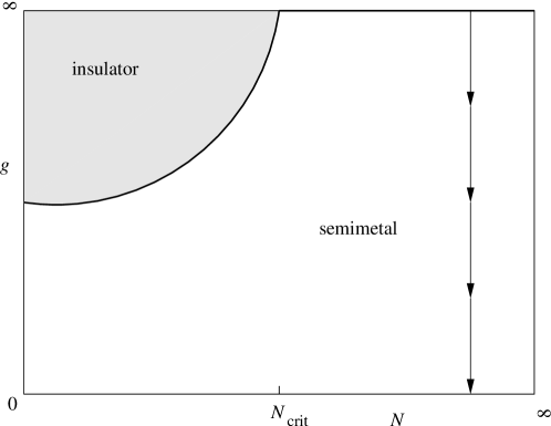
Figure 3: A slightly more complicated phase diagram. For $N>N_{\rm crit}$, the system is always in the semimetal phase. For $N<N_{\rm crit}$, it can be in the semimetal phase [for $g<g_{c}(N)$] or in the insulating phase [for $g>g_{c}(N)$].

If the phase diagram is as in Fig. 3, then two possibilities exist for real graphene. If $N_{\rm crit}<2$, or if $N_{\rm crit}>2$ but the bare Coulomb coupling (in vacuum) $g<g_{c}(N=2)$, then graphene is a semimetal. In contrast, if $N_{\rm crit}>2$ and in vacuum $g>g_{c}(N=2)$, then freely suspended graphene suspended is an insulator. All available experimental data, on the other hand, are consistent with graphene on a SiO₂ substrate being a semimetal. Therefore, if in vacuum graphene is insulating, then it undergoes an insulator-semimetal phase transition as a function of the dielectric constant of the substrate.

The authors of Refs. Gorbar:2002iw ; Leal:2003sg solved a gap equation with the screened Coulomb interaction and found $N_{\rm crit}\approx 2.55$. If this is the case, then the system with $N=2$ develops an excitonic gap at sufficiently large $g$. However, this result is probably not conclusive as the gap equation in Ref. Gorbar:2002iw ; Leal:2003sg is not systematic at small $N$, and also neglects the frequency dependence in the photon propagator. Ultimately, the phase diagram of graphene should (and could) be determined by a direct numerical simulation of the theory.

In the rest of this section, we shall assume that the phase diagram is as in Fig. 2, or as in Fig. 3 with $N_{\rm crit}<2$. The system with $N=2$ and infinite Coulomb coupling should show scale invariance (3) with a critical exponent $z$ which can be estimated by extrapolating Eq. (17),

$$z\approx 0.8\quad\textrm{for $N=2$}.$$ (32)

Note that the $1/N$ correction to $z$ is only $20\%$ at $N=2$, giving us hope that the $1/N$ expansion works reasonably well even for $N=2$.

The question now is whether in real graphene $\lambda$ is large enough so that the system is closed to the scale-invariant regime. If we take the typical experimental value $v=10^{6}~{}\textrm{m}/\textrm{s}$ Novoselov-Nature ; Kim-Nature then we find $\lambda\approx 3.4$, which is reasonably large compared to 1. Therefore, one concludes that graphene is sufficiently close to the scale-invariant regime. However, in most experiments the graphene single layer lies on a substrate, which reduces the effective Coulomb potential [Eq. (6)]. If we take the substrate to be SiO₂ with $\varepsilon=4.5$, we find $\lambda\approx 1.25$, which is only marginally larger than 1.

The above quoted value $\lambda\approx 3.4$ should be thought of as the initial condition for the RG equation, valid at the momentum scale of the order of the inverse lattice size. As we flow to the infrared, the system deviates more and more from the strongly coupled fixed point due to the bare kinetic term which is a relevant perturbation. However as the initial condition is relatively close to the fixed point, it will take a large “RG time” to go to the weak coupling regime $\lambda\ll 1$. The graphene thus remains close to the strong coupling limit for a large momentum range. The width of this range can be roughly estimated as

$$\exp\left(\frac{\pi^{2}N}{4}\ln 3.4\right)\sim 10^{3},$$ (33)

where we have used the leading $1/N$ result for the dimension of the bare Coulomb kinetic term.

An additional information for the effect of finite $\lambda$ can be obtained from the value of the anomalous dimension for the velocity as given by Eq. (14) at $\lambda=3.4$:

$$\gamma_{v}(3.4)\approx 0.7\gamma_{v}(\infty)\approx 0.15.$$ (34)

It is a 30% reduction of the anomalous dimension $\gamma_{v}$. In Fig. 1, we see that for the realistic $\lambda$ the different $f_{1}-f_{0}$ is already a rather flat function of $\lambda$; an approximate scaling behavior can be expected.

At the asymptotic infrared end of the RG flow is the trivial fixed point $\lambda=0$, near which the fermion velocity increases linearly with the logarithm of the momentum [as followed from Eq. (14) and the small $\lambda$ asymptotics in Eqs. (26)],

$$-p\frac{\partial v(p)}{\partial p}=\frac{g^{2}}{16\pi}\,,$$ (35)

which translates into an increase of $1.26\times 10^{6}~{}\textrm{m}/\textrm{s}$ per decade for graphene in vacuum. However, this regime is achieved only at extremely low momenta after the system has passed from the vicinity of the strongly coupled fixed point to the trivial one.

VI Conclusion

In this paper, we consider a model of $N$ massless four-component Dirac fermions interacting through an instantaneous Coulomb interaction. We show that in the limit of infinitely strong coupling, the system shows a scale-invariant behavior (3) which is characterized by a dynamic critical exponent $z$. We obtain the value of $z$ at large $N$.

We also discuss two possibilities for the phase diagram of the system at finite $N$. In one of the possibilities, a part of the phase diagram is occupied by the insulator phase. It is very interesting if in freely suspended graphene the Coulomb interaction is strong enough to open an excitonic gap. Provided that such a gap is never opened for $N=2$, we argue that the Coulomb interaction in vacuum is strong enough so that freely suspended graphene sheets can be considered as being in the vicinity of the strong-coupling fixed point for a large range of momentum.

How can our predictions be tested in experiment? Assume one could measure with high precision the quasiparticle dispersion curve in freely suspended graphene. If the strong-coupling large-$N$ limit is any guide, then one should have a slight deviation from the linear dispersion law, perhaps approximately $\omega\sim p^{0.85}$ [see Eq. (34)]. For graphene on a substrate, the deviation from the linear law is smaller.

Finally, we hope that this work will motivate numerical simulations of the model (5), which should help clarify it phase structure.

Appendix A Calculation of the beta function at large $N$

A.1 Coulomb propagator

To leading order in the large-$N$ expansion, we must resum all fermion bubble graphs in the Coulomb propagator. We shall perform calculations in the unit system where $v=1$ and restore $v$ in final formulas when needed.

Figure 4: The photon polarization diagram.

The one-loop fermion bubble diagram (Fig. 4) is

$$\Pi(q)=Ng^{2}\int\!\frac{d^{3}k}{(2\pi)^{3}}\,\textrm{Tr}\,\left(\gamma^{0}\frac{1}{{k\hskip-9.0pt\diagup}}\gamma^{0}\frac{1}{{k\hskip-9.0pt\diagup}+{q\hskip-7.0pt\diagup}}\right),$$ (36)

where ${k\hskip-9.0pt\diagup}=\gamma^{\mu}k_{\mu}$, $\mu=0,1,2$. The manipulation of the Dirac algebra proceeds in a standard fashion. We use the formulas

$$\frac{1}{{k\hskip-9.0pt\diagup}}=\frac{{k\hskip-9.0pt\diagup}}{k^{2}},$$ (37)

$$\textrm{Tr}\,(\gamma^{\mu}\gamma^{\nu}\gamma^{\rho}\gamma^{\sigma})=4(\delta^{\mu\nu}\delta^{\rho\sigma}-\delta^{\mu\rho}\delta^{\nu\sigma}+\delta^{\mu\sigma}\delta^{\nu\rho})$$ (38)

to find

$$\Pi(q)=4Ng^{2}\int\!\frac{d^{3}k}{(2\pi)^{3}}\,\frac{2k_{0}(k_{0}+q_{0})-k\cdot(k+q)}{k^{2}(k+q)^{2}}\,.$$ (39)

We now use Feynman parametrization

$$\frac{1}{AB}=\int_{0}^{1}\!dx\,\frac{1}{[xA+(1-x)B]^{2}}$$ (40)

to rewrite

$$\Pi(q)=4Ng^{2}\int_{0}^{1}\!dx\!\int\!\frac{d^{3}k}{(2\pi)^{3}}\,\frac{2k_{0}(k_{0}+q_{0})-k\cdot(k+q)}{[(1-x)k^{2}+x(k+q)^{2}]^{2}}\,.$$ (41)

Changing the integration varibale $k\to k-xq$, the denominator in the integrand becomes an even function of $q$, and one can throw away terms odd in $k$ in the numerator. Furthermore due to spherical symmetry we can replace in the numerator $k_{0}^{2}\to k^{2}/3$. We find

$$\Pi(q)=4Ng^{2}\int_{0}^{1}\!dx\!\int\!\frac{d^{3}k}{(2\pi)^{3}}\,\frac{-\tfrac{1}{3}k^{2}-2x(1-x)q_{0}^{2}-x(1-x)q^{2}}{[k^{2}+x(1-x)q^{2}]^{2}}\,.$$ (42)

We perform integration over $k$ using standard formulas of dimensional regularization

$$\int\!\frac{d^{d}k}{(2\pi)^{d}}\,\frac{1}{(k^{2}+\Delta)^{n}} =\frac{1}{(4\pi)^{d/2}}\,\frac{\Gamma(n-\frac{d}{2})}{\Gamma(n)}\,\frac{1}{\Delta^{n-d/2}}\,,$$ (43)

$$\int\!\frac{d^{d}k}{(2\pi)^{d}}\,\frac{k^{2}}{(k^{2}+\Delta)^{n}} =\frac{1}{(4\pi)^{d/2}}\,\frac{d}{2}\,\frac{\Gamma(n-\frac{d}{2}-1)}{\Gamma(n)}\,\frac{1}{\Delta^{n-d/2-1}}$$ (44)

to obtain

$$\Pi(q)=\frac{g^{2}N}{\pi}\frac{|{\vec{q}}|^{2}}{\sqrt{q^{2}}}\int\!dx\,[x(1-x)]^{1/2}=\frac{g^{2}N}{8}\frac{{\vec{q}}^{2}}{\sqrt{q_{0}^{2}+v^{2}|{\vec{q}}|^{2}}}\,,$$ (45)

where in the last expression we have restored $v$. The resummed Coulomb propagator is

$$D(q)=\left(2|{\vec{q}}|+\frac{g^{2}N}{8}\frac{|{\vec{q}}|^{2}}{\sqrt{q^{2}}}\right)^{-1}$$ (46)

A.2 Correction to fermion propagator

We now compute the $1/N$ correction to the fermion self-energy (Fig. 5):

$$\Sigma(p)=-g^{2}\int\!\frac{d^{3}q}{(2\pi)^{3}}\,\frac{\gamma^{0}({p\hskip-7.0pt\diagup}-{q\hskip-7.0pt\diagup})\gamma^{0}}{(p-q)^{2}}D(q).$$ (47)

Figure 5: The fermion self-energy diagram.

The integral is naively linearly divergent at large $q$, but to leading order in $q$ the integrand is an odd function of $q$. Therefore, the integral is only logarithmically divergent and can be evaluated by expanding in $p\ll q$. One finds

$$\Sigma(p)=Z_{0}\gamma^{0}p_{0}+Z_{1}\gamma^{i}p_{i},$$ (48)

where

$$Z_{0} =g^{2}\int\!\frac{d^{3}q}{(2\pi)^{3}}\,\frac{q_{0}^{2}-|{\vec{q}}|^{2}}{q^{4}}D(q),$$ (49)

$$Z_{1} =g^{2}\int\!\frac{d^{3}q}{(2\pi)^{3}}\,\frac{q_{0}^{2}}{q^{4}}D(q).$$ (50)

Introducing spherical coordinates: $q_{0}=q\cos\theta$, $|{\vec{q}}|=q\sin\theta$, one can then write

$$Z_{0} =\frac{4}{\pi^{2}N}\,\frac{\lambda}{2}\int\limits_{0}^{\pi}\!\sin\theta\,d\theta\,\frac{\cos^{2}\theta-\sin^{2}\theta}{\sin\theta(1+\lambda\sin\theta)}\int\!\frac{dq}{q}\,,$$ (51)

$$Z_{1} =\frac{4}{\pi^{2}N}\,\frac{\lambda}{2}\int\limits_{0}^{\pi}\!\sin\theta\,d\theta\,\frac{\cos^{2}\theta}{\sin\theta(1+\lambda\sin\theta)}\int\!\frac{dq}{q}\,,$$ (52)

where $\lambda=g^{2}N/16$. The integral over $dq$ in a spherical shell $\Lambda_{1}<q<\Lambda_{0}$ yields $\ln(\Lambda_{0}/\Lambda_{1})$. The angular integral can be taken explicitly and results in Eqs. (20), (22), and (23).

References

- (1) K. S. Novoselov, D. Jiang, F. Schedin, T. J. Booth, V. V. Khotkevich, S. V. Morozov, and A. K. Geim, “Two dimensional atomic crystals,” Proc. Natl. Acad. Sci. U.S.A. 102, 10451 (2005) [arXiv:cond-mat/0503533].
- (2) G. W. Semenoff, “Condensed matter simulation of a three-dimensional anomaly,” Phys. Rev. Lett. 53, 2449 (1984).
- (3) K. S. Novoselov, A. K. Geim, S. V. Morozov, D. Jiang, M. I. Katsnelson, I. V. Grigorieva, S. V. Dubonos, and A. A. Firson, “Two-dimensional gas of massless Dirac fermions in graphene,” Nature (London) 438, 197 (2005) [arXiv:cond-mat/0509330].
- (4) Y. Zhang, Y.-W. Tan, H. L. Stormer, and P. Kim, “Experimental observation of the quantum Hall effect and Berry’s phase in graphene,” Nature (London) 438, 201 (2005) [arXiv:cond-mat/0509355].
- (5) V. P. Gusynin and S. G. Sharapov, “Unconventional integer quantum Hall effect in graphene,” Phys. Rev. Lett. 95, 146801 (2005) [arXiv:cond-mat/0506575].
- (6) S. Sachdev, Quantum Phase Transitions (Cambridge University Press, Cambridge, 1999).
- (7) H. B. Nielsen and M. Ninomiya, “Absence of neutrinos on a lattice. 1. Proof by homotopy theory,” Nucl. Phys. B 185, 20 (1981) [Erratum-ibid. B 195, 541 (1982)].
- (8) H. B. Nielsen and M. Ninomiya, “Absence of neutrinos on a lattice. 2. Intuitive topological proof,” Nucl. Phys. B 193, 173 (1981).
- (9) J. Ye and S. Sachdev, “Coulomb interactons at quantum Hall critical points of systems in a periodic potential,” Phys. Rev. Lett. 80, 5409 (1998) [arXiv:cond-mat/9712161].
- (10) J. C. Meyer, A. K. Geim, M. I. Katsnelson, K. S. Novoselov, T. J. Booth, S. Roth, “The structure of suspended graphene sheets,” Nature (London) 446, 60 (2007) [arXiv:cond-mat/0701379].
- (11) I. F. Herbut, “Interactions and phase transitions on graphene’s honeycomb lattice,” Phys. Rev. Lett. 97, 146401 (2006) [arXiv:cond-mat/0606195].
- (12) S. Templeton, “Summation of dominant coupling constant logarithms in QED in three-dimensions,” Phys. Lett. B 103, 134 (1981).
- (13) S. Templeton, “Summation of coupling constant logarithms in QED in three-dimensions,” Phys. Rev. D 24, 3134 (1981).
- (14) T. Appelquist, D. Nash, and L. C. R. Wijewardhana, “Critical behavior in (2+1)-dimensional QED,” Phys. Rev. Lett. 60, 2575 (1988).
- (15) J. González, F. Guinea, and M. A. H. Vozmediano, “Non-Fermi liquid behavior of electrons in the half filled honeycomb lattice (a renormalization group approach),” Nucl. Phys. B 424, 595 (1994) [arXiv:hep-th/9311105].
- (16) J. González, F. Guinea, and M. A. H. Vozmediano, “Marginal-Fermi-liquid behavior from two-dimensional Coulomb interaction,” Phys. Rev. B 59, R2474 (1999) [arXiv:cond-mat/9807130].
- (17) I. F. Herbut, “Quantum critical points with the Coulomb interaction and the dynamic exponent: when and why ,” Phys. Rev. Lett. 87, 137004 (2001) [arXiv:cond-mat/0105544].
- (18) O. Vafek, “Specific heat of massless Dirac fermions with Coulomb interactions in two spatial dimensions,” Phys. Rev. Lett. 98, 216401 (2007) [arXiv:cond-mat/0701145].
- (19) N. M. R. Peres, F. Guinea, and A. H. Castro Neto, “ Coulomb interactions and ferromagnetism in pure and doped graphene,” Phys. Rev. B 72, 174406 (2005).
- (20) J. Nilsson, A. H. Castro Neto, N. M. R. Peres, and F. Guinea, “ Electron-electron interactions and the phase diagram of a graphene bilayer,” Phys. Rev. B 73, 214418 (2006).
- (21) E. V. Gorbar, V. P. Gusynin, V. A. Miransky, and I. A. Shovkovy, “Magnetic field driven metal-insulator phase transition in planar systems,” Phys. Rev. B 66, 045108 (2002) [arXiv:cond-mat/0202422].
- (22) H. Leal and D. V. Khveshchenko, “Excitonic instability in two-dimensional degenerate semimetals, Nucl. Phys. B 687, 323 (2004) [arXiv:cond-mat/0302164].