Fractional Spin Hall Effect in Atomic Bose Gases

Abstract

We propose fractional spin hall effect (FSHE) by coupling pseudospin states of cold bosonic atoms to optical fields. The present scheme is an extension to interacting bosonic system of the recent work liu ; zhu on optically induced spin hall effect in non-interacting atomic system. The system has two different types of ground states. The 1st type of ground state is a $1/3$-factor Laughlin function, and has the property of chiral - anti-chiral interchange antisymmetry, while the 2nd type is shown to be a $1/4$-factor wave function with chiral - anti-chiral symmetry. The fractional statistics corresponding to the fractional spin Hall states are studied in detail, and are discovered to be different from that corresponding to the fractional quantum Hall (FQH) states. Therefore the present FSHE can be distinguished from FQH regime in the measurement.

I Introduction

Intrinsic spin Hall effect (SHE) has attracted great attention since it was predicted in semiconductors with spin-orbit coupled structures SHE1 ; SHE2 ; SHE3 ; graphene , with the concomitant creation of spin currents and realization of quantized spin hall conductance (SHC). Quantum SHE with non-interacting particles was firstly studied in graphene graphene1 ; graphene2 and semiconductors with a strain gradient structure zhang2 , while by now there are no experimental systems available for such proposals. Recently, Bernevig, Hughes and Zhang theoretically predicted the quantum SHE in HgTe/CdTe quantum wells zhang1 . By varying the thickness of the quantum well, a quantum phase transition is obtained between the conventional insulator and the quantum spin Hall (QSH) insulator. Such a prediction has been remarkably confirmed in the recent experiment experiment1 . The QSH insulator is a topologically nontrivial state of matter protected by the time reversal symmetry, and it is currently described through a $Z_{2}$ classification graphene1 ; graphene2 ; Z2 . Considering the nontrivial topological properties, such QSH insulators may have not only potential applications and but also the fundamental importance in physics.

On the other hand, the similar idea for the SHE has been proposed in cold non-interacting atomic system by coupling the internal atomic states (atomic spins) to radiation liu ; zhu . The atom-light coupling creates a spin-dependent effective magnetic field, leading to SHE in fermionic atomic systems. A challenging but interesting extension is the realization of fractional spin Hall (FSH) regime with the particle-particle interactions considered. The correlated many-body function in the FSH regime was initially described in the Ref. zhang2 . Nevertheless, many issues are left in the fractional spin Hall effect (FSHE), e.g. the fractional statistics corresponding to the FSH state is not clear and needs to be further investigated. Comparing with solid matters, ultra-cold atomic system provides a unique access to the study of complex many-body dynamics with its extremely clean environment and remarkable controllability in the parameters. Therefore it is very suggestive to study the FSHE by extending optically induced SHE liu ; zhu to interacting bosonic atomic systems where, different from former schemes with the non-interacting atomic gas, the nonlinear interaction between atoms (s-wave scattering) plays a central role in the Hall effect.

In this paper, we propose FSHE by coupling internal electronic states of cold bosonic atoms to the external optical fields, with atom-atom interaction considered. Under the lowest Landau level (LLL) condition, we can exactly study the ground states of the present many-body system. The intriguing fundamental properties of FSH states and the corresponding fractional statistics in our system are investigated.

The paper is organized as follow. In section II, we derive the effective Hamiltonian that gives FSHE. Then in section III, we study the FSH state and corresponding quasi-particle excitation, with which we point out differences between the present FSH regime and the fractional quantum Hall (FQH) regime. Realization of the FSHE in realistic atomic systems is discussed in section IV. Finally we conclude our results in section V.

II Effective Hamiltonian

In this section we shall study two different configurations to obtain the effective Hamiltonian that gives the FSHE in the cold atoms.

II.1 Four-level configuration

We first consider the four-level configuration shown in Fig. 1(a). An ensemble of cold bosonic atoms with four internal angular momentum states (atomic spins), described by atomic state functions $\Phi_{\alpha}(\mathbb{r},t)$ ($\alpha=e_{\pm},s_{\pm}$), interact with two external light fields.

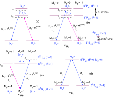
Figure 1: (color online) (a) Four-level bosonic atoms interacting with two light fields; This case can be experimentally realized with e.g. ⁸⁷Rb atoms ((b) and (c) ); (d) Initial condition achieved by pumping the atoms into $|S_{\pm}\rangle$ with $|\Omega_{+}|=|\Omega_{-}|$ through the $\Lambda$-type configuration.

The transitions from $|s_{\pm}\rangle$ to $|e_{\pm}\rangle$ are respectively coupled by a $\sigma_{-}$ light with the Rabi-frequency $\Omega_{1}=\Omega_{10}\exp(i(\mathbb{k}_{1}\cdot\mathbb{r}+l_{1}\vartheta))$ and by a $\sigma_{+}$ light with the Rabi-frequency $\Omega_{2}=\Omega_{20}\exp(i(\mathbb{k}_{2}\cdot\mathbb{r}+l_{2}\vartheta))$, where $\mathbb{k}_{1,2}=k_{1,2}\mathbb{\hat{e}}_{z}$ and $\vartheta=\tan^{-1}({y}/{x})$. $l_{1}$ and $l_{2}$ indicate that $\sigma_{+}$ and $\sigma_{-}$ photons respectively have the orbital angular momenta $\hbar l_{1}$ and $\hbar l_{2}$ along the $+z$ direction angular . It is convenient to introduce the slowly-varying amplitudes of atomic wave-functions by (note $\omega_{s_{\pm}}=0$): $\phi_{s_{\pm}}=\Phi_{s_{\pm}},\phi_{e_{+}}=\Phi_{e_{+}}(\mathbb{r},t)e^{-i(\mathbb{k}_{1}\cdot\mathbb{r}-(\omega_{e_{+}}-\Delta_{1})t)},\phi_{e_{-}}=\Phi_{e_{-}}(\mathbb{r},t)e^{-i(\mathbb{k}_{2}\cdot\mathbb{r}-(\omega_{e_{-}}-\Delta_{2})t)}$, where $\hbar\omega_{\alpha}$ is the energy of the state $|\alpha\rangle$, $\Delta_{1}$ and $\Delta_{2}$ are transition detunings. The total Hamiltonian of the present system can be written as $H=H_{0}+H_{1}+H_{2}$, with

$$H_{0} = \sum_{\alpha=e_{\pm},s_{\pm}}\int d^{3}r\phi_{\alpha}^{*}\bigl{(}-\frac{\hbar^{2}}{2m}\nabla^{2}+V(\mathbb{r})\bigl{)}\phi_{\alpha}$$

$$+ \sum_{\alpha,\beta}\int d^{3}rd^{3}r^{\prime}\phi_{\alpha}^{*}(\mathbb{r})\phi_{\beta}^{*}(\mathbb{r}^{\prime})U_{\alpha\beta}(\mathbb{r},\mathbb{r}^{\prime})\phi_{\alpha}(\mathbb{r})\phi_{\beta}(\mathbb{r}^{\prime}),$$

$$H_{1} = \hbar\Delta_{1}\int d^{3}r\phi^{*}_{e_{+}}S_{e_{+}e_{+}}\phi_{e_{+}}$$ (1)

$$-\hbar\int d^{3}r(\phi^{*}_{e_{+}}\Omega_{10}e^{il_{1}\vartheta}S_{1+}\phi_{s_{+}}+h.a.),$$

$$H_{2} = \hbar\Delta_{2}\int d^{3}r\phi^{*}_{e_{-}}S_{e_{-}e_{-}}\phi_{e_{-}}$$

$$-\hbar\int d^{3}r(\phi^{*}_{e_{-}}\Omega_{20}e^{il_{2}\vartheta}S_{2+}\phi_{s_{-}}+h.a.),$$

with the atomic operators defined by $S_{e_{\pm}e_{\pm}}=|e_{\pm}\rangle\langle e_{\pm}|$, $S_{1+}=|e_{+}\rangle\langle s_{+}|,S_{2+}=|e_{-}\rangle\langle s_{-}|$ and $S^{{\dagger}}_{\alpha+}=S_{\alpha-}$. $V(\mathbb{r})$ is the external trap potential. The s-wave scattering potential is characterizes via $U_{\alpha\beta}(\mathbb{r})=(4\pi\hbar^{2}a_{\alpha\beta}/m)\delta^{(3)}(\mathbb{r}-\mathbb{r}^{\prime})$ with $a_{\alpha\beta}$ the scattering length.

The interaction Hamiltonian $(H_{1}+H_{2})$ can be diagonalized with a local unitary transformation. Similar to the former results liu , here we consider the large detuning case i.e. $\Delta_{j}^{2}\gg\Omega_{j0}^{2}$. In this way, spontaneous emission is suppressed by introducing the adiabatic condition sun that the population of the higher levels is adiabatically eliminated, and the total system is restricted to the two ground states $|S_{-}\rangle$ and $|S_{+}\rangle$. Under the present adiabatic condition the Hamiltonian (II.1) can be written in an effective form which involves only the two ground states:

$$H = \int d^{3}r\phi_{s_{-}}^{*}\bigr{[}\frac{1}{2m}(i\hbar\partial_{k}+\frac{e}{c}A_{k})^{2}+V_{-}(\mathbb{r})\bigr{]}\phi_{s_{-}}$$ (2)

$$+ \int d^{3}r\phi_{s_{+}}^{*}\bigr{[}\frac{1}{2m}(i\hbar\partial_{k}-\frac{e}{c}A_{k})^{2}+V_{+}(\mathbb{r})\bigr{]}\phi_{s_{+}}$$

$$+ \sum_{\mu,\nu=+,-}\int d^{3}rd^{3}r^{\prime}\phi_{s_{\mu}}^{*}(\mathbb{r})\phi_{s_{\nu}}^{*}(\mathbb{r}^{\prime})U_{\mu\nu}(\mathbb{r},\mathbb{r}^{\prime})\times$$

$$\times\phi_{s_{\mu}}(\mathbb{r})\phi_{s_{\nu}}(\mathbb{r}^{\prime}).$$

Here the vector and scalar potentials induced by the atom-light couplings are liu : $\mathbb{A}_{-}=-\mathbb{A}_{+}=\mathbb{A}=\hbar lce^{-1}\frac{\Omega_{0}^{2}}{\Delta^{2}}(x\hat{e}_{y}-y\hat{e}_{x})/\rho^{2}$ and (neglecting constant terms) $V_{\pm}(\mathbb{r})=V_{eff}(\mathbb{r})=V(\mathbb{r})-\hbar\Omega^{2}_{0}/\Delta-\hbar^{2}l^{2}\Omega_{0}^{4}/(2m\Delta^{4}\rho^{2})$ with $\rho=\sqrt{x^{2}+y^{2}}$. In the above calculations we have set $\Delta_{1}=\Delta_{2}=\Delta$, $\Omega_{10}=\Omega_{20}=\Omega_{0}$ and $l_{1}=-l_{2}=l$, i.e. the angular momenta of the two light fields are opposite in direction. Generally, we assume the total atomic number is $N=N_{+}+N_{-}$, where $N_{\pm}$ are the numbers of atoms in states $|S_{\pm}\rangle$. To facilitate further discussion, we describe here the effective Hamiltonian in the $N$-particle case:

$$H = \sum_{j=1}^{N_{+}}\bigr{[}\frac{1}{2m}\bigl{(}P^{+j}_{k}+\frac{e}{c}A_{k}(\mathbb{r}^{+}_{j})\bigl{)}^{2}+V_{eff}(\mathbb{r}^{+}_{j})\bigr{]}$$ (3)

$$+ \sum_{j=1}^{N_{-}}\bigr{[}\frac{1}{2m}\bigl{(}P^{-j}_{k}-\frac{e}{c}A_{k}(\mathbb{r}^{-}_{j})\bigl{)}^{2}+V_{eff}(\mathbb{r}^{-}_{j})\bigr{]}$$

$$+ \sum_{j<k}\sum_{\alpha,\beta=+,-}(4\pi\hbar^{2}a_{\alpha\beta}/m)\delta^{(3)}(\mathbb{r}^{\alpha}_{j}-\mathbb{r}^{\beta}_{k}).$$

For convenience, in this paper we shall consider the spin-independent s-wave scattering, say, $a_{\alpha\beta}=a\equiv const.$, independent of $\alpha,\beta$. Practically, we apply two columnar spreading light fields that $\Omega_{01}(\mathbb{r})=\Omega_{02}(\mathbb{r})=f\rho$ with the coefficient $f>0$. This kind of fields can be created by e.g. high order Bessel beams angular . Further, we set a two-dimensional harmonic trap by $V(\mathbb{r})=\frac{1}{2}m\omega^{2}_{\perp}\rho^{2}$, so the scalar potential reads $V_{eff}(\mathbb{r})=\frac{1}{2}m\omega^{2}_{eff}\rho^{2}$, where $\omega^{2}_{eff}=\omega^{2}_{\perp}-(1+\frac{\hbar l^{2}f^{2}}{2m\Delta^{3}})\frac{2\hbar f^{2}}{m\Delta}$. Note the atomic numbers in spin-up and spin-down states are determined by initial condition that can be controlled in experiment. Here we would like to assume $N_{\pm}=N/2$. Finally, we can apply a tight harmonic confinement along $z$-axis with frequency $\omega_{z}$ such that $z$-axial ground state energy far exceeds any other transverse energy scale, yielding a quasi-2D system LLL . With these considerations we can further obtain the effective Hamiltonian by

$$H = \sum_{j=1}^{N/2}\frac{1}{2m}\bigl{(}\mathbb{P}^{+j}+\frac{eB}{2c}\hat{\mathbb{e}}_{z}\times\mathbb{r}^{+}_{j}\bigl{)}^{2}+H_{L}^{+}$$ (4)

$$+ \sum_{j=1}^{N/2}\frac{1}{2m}\bigl{(}\mathbb{P}^{-j}-\frac{eB}{2c}\hat{\mathbb{e}}_{z}\times\mathbb{r}^{-}_{j})\bigl{)}^{2}+H_{L}^{-}$$

$$+ \sum_{j<k}\sum_{\alpha,\beta=+,-}\tilde{g}\delta^{(2)}(\mathbb{r}^{\alpha}_{j}-\mathbb{r}^{\beta}_{k}).$$

Here $\tilde{g}=a\sqrt{8\pi\hbar^{3}\omega_{z}^{2}/m}$ is the 2D interaction strength, the angular momentum part reads

$$H_{L}^{\pm}=\pm(1-\Theta)eBL_{z}^{\pm}/4mc$$ (5)

with the total angular momenta of atoms in spin states $|S_{\pm}\rangle$: $L_{z}^{\pm}=\sum_{j=1}^{N/2}L_{jz}^{\pm}$ and $\Theta=(1+\frac{4m^{2}\Delta^{4}\omega_{eff}^{2}}{\hbar^{2}l^{2}f^{4}})^{-1/2}$ equivalent to the “rotation rate” of fractional quantum Hall effect (FQHE) in rotating bosonic systems Cornell ; FQHE1 ; FQHE2 ; FQHE that has been widely studied in recent years, and

$$B=\frac{\hbar lc}{e}\frac{f^{2}}{\Delta^{2}}\bigr{(}1+\frac{4m^{2}\Delta^{2}\omega_{eff}^{2}}{\hbar^{2}l^{2}f^{4}}\bigr{)}^{\frac{1}{2}}$$ (6)

characterizes the optically induced magnetic field. From the formula (4) one can see the key difference between our model and FQHE in the rotating BECs Cornell ; FQHE1 ; FQHE2 ; FQHE is that here atoms experience $spin$-$dependent$ effective magnetic fields ($\mathbb{B}_{-}=-\mathbb{B}_{+}=B\hat{\mathbb{e}}_{z}$). In the rotating bosonic atomic system, even the atomic spin degree is considered, all different spin states are in the same rotating direction, thus experience only a single (spin-independent) effective magnetic field. It is also noteworthy that the charge hall effect system or rotating bosonic atomic system is $P$-invariant but $T$-breaking. However, our system is both $P$- and $T$-invariant.

II.2 Double $\Lambda$-type configuration

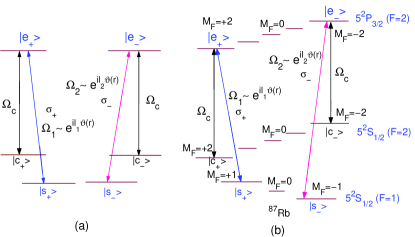
Figure 2: (color online) (a) Double $\Lambda$-type bosonic atoms interacting with two light fields ($\Omega_{1,2}$) with orbital angular momentum and one strong field $\Omega_{c}$; (b) This situation can be experimentally realized with e.g. ⁸⁷Rb atoms. Zeeman splitting is considered.

In this subsection we consider another situation, say the double $\Lambda$-type configuration (see Fig. 2 (a)) to reach the effective Hamiltonian (4). The transitions from $|s_{\pm}\rangle$ to $|e_{\pm}\rangle$ are respectively coupled by a $\sigma_{+}$ light with the Rabi-frequency $\Omega_{1}=\Omega_{10}\exp(i(\mathbb{k}_{1}\cdot\mathbb{r}+l_{1}\vartheta))$ and by a $\sigma_{-}$ light with the Rabi-frequency $\Omega_{2}=\Omega_{20}\exp(i(\mathbb{k}_{2}\cdot\mathbb{r}+l_{2}\vartheta))$, where $\mathbb{k}_{1,2}=k_{1,2}\mathbb{\hat{e}}_{z}$ and $\vartheta=\tan^{-1}({y}/{x})$. Different from the former situation, here the couplings are resonant. Besides, we apply the third strong $\pi$ laser field with $\Omega_{c}=\Omega_{c0}\exp(i\mathbb{k}_{c}\cdot\mathbb{r})$ that couples both transitions from $|c_{+}\rangle$ to $|e_{+}\rangle$ and from $|c_{+}\rangle$ to $|e_{+}\rangle$. Also, we introduce the slowly-varying amplitudes of atomic wave-functions by: $\phi_{s_{\pm}}=\Phi_{s_{\pm}}$, $\phi_{e_{\pm}}=\Phi_{e_{\pm}}(\mathbb{r},t)e^{-i(\mathbb{k}_{1,2}\cdot\mathbb{r}-\omega_{e_{\pm}}t)}$, $\phi_{c_{\pm}}=\Phi_{c_{\pm}}(\mathbb{r},t)e^{-i[(\mathbb{k}_{1,2}-\mathbb{k}_{c})\cdot\mathbb{r}-\omega_{c_{\pm}}]t}$. The total Hamiltonian of the present system $H=H_{0}+H_{\Lambda_{1}}+H_{\Lambda_{2}}$ is given by

$$H_{0} = \sum_{\alpha=e_{\pm},s_{\pm},c_{\pm}}\int d^{3}r\phi_{\alpha}^{*}\bigl{(}-\frac{\hbar^{2}}{2m}\nabla^{2}+V(\mathbb{r})\bigl{)}\phi_{\alpha}$$

$$+ \sum_{\alpha,\beta}\int d^{3}rd^{3}r^{\prime}\phi_{\alpha}^{*}(\mathbb{r})\phi_{\beta}^{*}(\mathbb{r}^{\prime})U_{\alpha\beta}(\mathbb{r},\mathbb{r}^{\prime})\phi_{\alpha}(\mathbb{r})\phi_{\beta}(\mathbb{r}^{\prime}),$$

$$H_{\Lambda_{1}} = -\hbar\int d^{3}r(\phi^{*}_{e_{+}}\Omega_{10}e^{il_{1}\vartheta}S_{e_{+}s_{+}}\phi_{s_{+}}+h.a.)$$ (7)

$$-\hbar\int d^{3}r(\phi^{*}_{e_{+}}\Omega_{c0}S_{e_{+}c_{+}}\phi_{c_{+}}+h.a.),$$

$$H_{\Lambda_{2}} = -\hbar\int d^{3}r(\phi^{*}_{e_{-}}\Omega_{20}e^{il_{2}\vartheta}S_{e_{-}s_{-}}\phi_{s_{-}}+h.a.)$$

$$-\hbar\int d^{3}r(\phi^{*}_{e_{-}}\Omega_{c0}S_{e_{-}c_{-}}\phi_{c_{-}}+h.a.).$$

It is easy to check that both $H_{\Lambda_{1}}$ and $H_{\Lambda_{2}}$ have three eigenstates, i.e. one dark state and two bright states darkstate1 ; darkstate2 : $|D_{1}\rangle=\cos\theta_{1}|s_{+}\rangle-\sin\theta_{2}e^{-il_{1}\vartheta}|c_{+}\rangle$, $|B_{1\pm}\rangle=\bigr{[}|e_{+}\rangle\pm(\sin\theta_{1}|s_{+}\rangle+\cos\theta_{2}e^{-il_{1}\vartheta}|c_{+}\rangle)\bigr{]}/\sqrt{2}$ for $H_{\Lambda_{1}}$ and $|D_{2}\rangle=\cos\theta_{2}|s_{+}\rangle-\sin\theta_{2}e^{-il_{2}\vartheta}|c_{+}\rangle$, $|B_{2\pm}\rangle=\bigr{[}|e_{+}\rangle\pm(\sin\theta_{2}|s_{+}\rangle+\cos\theta_{2}e^{-il_{2}\vartheta}|c_{+}\rangle)\bigr{]}/\sqrt{2}$ for $H_{\Lambda_{2}}$, where the mixing angles are defined via $\tan\theta_{1,2}=|\Omega_{1,2}|/\Omega_{c0}$. The corresponding eigenvalues are $E_{D_{1,2}}=0$, $E_{B_{1\pm}}=\pm\sqrt{\Omega_{c0}^{2}+\Omega_{10}^{2}}$ and $E_{B_{2\pm}}=\pm\sqrt{\Omega_{c0}^{2}+\Omega_{20}^{2}}$. For our purpose we require the full system is trapped in the dark-state subspace $|D_{1,2}\rangle$ (a pseudospin-$1/2$ space), which excludes the excited states. This can be achieved when the laser fields are sufficiently strong so that the eigenvalues of the bright states are far separated from that of the two dark states. Under this condition the Hamiltonian (II.2) can be written in the effective form which involves only the two dark states:

$$H = \int d^{3}r\phi_{D_{1}}^{*}\bigr{[}\frac{1}{2m}(i\hbar\partial_{k}+\frac{e}{c}A_{1k})^{2}+V_{1}(\mathbb{r})\bigr{]}\phi_{D_{1}}$$ (8)

$$+ \int d^{3}r\phi_{D_{2}}^{*}\bigr{[}\frac{1}{2m}(i\hbar\partial_{k}+\frac{e}{c}A_{2k})^{2}+V_{2}(\mathbb{r})\bigr{]}\phi_{D_{2}}$$

$$+ \sum_{\mu,\nu=1,2}\int d^{3}rd^{3}r^{\prime}\phi_{D_{\mu}}^{*}(\mathbb{r})\phi_{D_{\nu}}^{*}(\mathbb{r}^{\prime})U_{\mu\nu}(\mathbb{r},\mathbb{r}^{\prime})\times$$

$$\times\phi_{D_{\mu}}(\mathbb{r})\phi_{D_{\nu}}(\mathbb{r}^{\prime}).$$

Here the vector potentials are calculated by $\mathbb{A}_{1,2}=i\hbar c/e\langle D_{1,2}|\nabla|D_{1,2}\rangle=\hbar l_{1,2}ce^{-1}\sin^{2}\theta_{1,2}(x\hat{e}_{y}-y\hat{e}_{x})/\rho^{2}$. Similar as before, we set $l_{1}=-l_{2}=l$ and $\Omega_{01}(\mathbb{r})=\Omega_{02}(\mathbb{r})=f\rho$, while $\Omega_{c0}$ is constant satisfying $\Omega_{c0}^{2}\gg|\Omega_{1,2}|^{2}$. Under this condition one can find the dark states $|D_{1,2}\rangle\approx|s_{\pm}\rangle$ and the vector potentials are followed by $\mathbb{A}_{2}=-\mathbb{A}_{1}=\mathbb{A}=\hbar f^{2}lce^{-1}\Omega_{c0}^{-2}(x\hat{e}_{y}-y\hat{e}_{x})$. Accordingly, the scalar potentials are obtained by $V_{1,2}(\mathbb{r})=V_{eff}(\mathbb{r})\approx V(\mathbb{r})-\hbar^{2}l^{2}f^{4}/(2m\Omega_{c0}^{4})$.

Though a straightforward generalization from the three-level $\Lambda$ configuration lambda1 ; lambda2 , the nontrivialness of the present double $\Lambda$ bosonic system with spin-dependent gauge field is protected by the result of quantum SHE whose integer version is identified to be of $Z_{2}$ topology graphene1 ; graphene2 . Again, we consider the spin-independent s-wave scattering, say, $a_{\mu\nu}=a\equiv const.$, and equal numbers of atoms ($N_{1}=N_{2}=N/2$) in the states $|D_{1,2}\rangle$. When a tight harmonic confinement is applied along $z$-axis, we can rewrite the above effective Hamiltonian by

$$H = \sum_{j=1}^{N/2}\frac{1}{2m}\bigl{(}\mathbb{P}_{1j}+\frac{eB}{2c}\hat{\mathbb{e}}_{z}\times\mathbb{r}_{1j}\bigl{)}^{2}+H_{1L}$$ (9)

$$+ \sum_{j=1}^{N/2}\frac{1}{2m}\bigl{(}\mathbb{P}_{2j}-\frac{eB}{2c}\hat{\mathbb{e}}_{z}\times\mathbb{r}_{2j})\bigl{)}^{2}+H_{2L}$$

$$+ \sum_{j<k}\sum_{\alpha,\beta=1,2}\tilde{g}\delta^{(2)}(\mathbb{r}^{\alpha}_{j}-\mathbb{r}^{\beta}_{k}).$$

The parameters in above formula can be similarly obtained as done in Eqs. (5) and (6), say $\tilde{g}=a\sqrt{8\pi\hbar^{3}\omega_{z}^{2}/m}$, the angular momentum part $H_{1L,2L}=\pm(1-\Theta)eBL_{z}^{\pm}/4mc$ with the total angular momenta of atoms in pseudospin states $|D_{1,2}\rangle$: $L_{z}^{\pm}=\sum_{j=1}^{N/2}L_{jz}^{\pm}$ and $\Theta=(1+\frac{4m^{2}\Omega_{c0}^{4}\omega_{eff}^{2}}{\hbar^{2}l^{2}f^{4}})^{-1/2}$, and $B=\frac{\hbar lc}{e}\frac{f^{2}}{\Omega_{c0}^{2}}\bigr{(}1+\frac{4m^{2}\Omega_{c0}^{2}\omega_{eff}^{2}}{\hbar^{2}l^{2}f^{4}}\bigr{)}^{\frac{1}{2}}$. It is clear that the effective Hamiltonian (9) is equivalent to that obtained in Eq. (4).

III FSH state and quasi-particle excitation

Atoms in different spin states experience the opposite magnetic fields $\mathbb{B}_{\alpha}$. This leads to a Landau level structure for each spin orientation. Together with the nonlinear interactions between spin states, the Hamiltonian (4) or (9) describes a FSHE in the bosonic system.

III.1 FSH state

In this subsection we shall first derive the FSH states for our system, and then in the next one discuss the related quasi-particle excitation. For this we consider the large optical angular momentum condition so that $\omega_{eff}\ll\omega=eB/mc$, then we approach the limit $\Theta\rightarrow 1$, which, in fact, corresponds to the fast rotating condition in usual bosonic atomic systems. In this way, the energy scales characterizing Hamiltonian $H_{L}^{\pm}$ are much smaller than those corresponding to other parts of $H$. Besides, we consider the case that atomic interaction energy is smaller than the energy spacing between two neighbor Landau levels. The two restrictions lead to LLL condition in our system (we shall return to the validity of this approximation later). The ground state and elementary excitations of (4) will then lie on the subspace of common zero energy eigenstates of $H-H_{L}^{\pm}$ FQHE1 ; FQHE2 . For this we can write down the many-body function of the present system as:

$$\Psi(z,\varpi^{*}) = {\cal P}(z_{1},z_{2},...,z_{N/2};\varpi_{1}^{*},\varpi_{2}^{*},...,\varpi_{N/2}^{*})\times$$ (10)

$$\times\prod_{j,k}e^{-|z_{j}|^{2}/2-|\varpi_{k}|^{2}/2},$$

where $z=x^{+}+iy^{+}$, $\varpi=x^{-}+iy^{-}$ are respectively the coordinates of atoms in states $|S_{+}\rangle$ and $|S_{-}\rangle$, and ${\cal P}(z;\varpi^{*})$ is a polynomial in all atomic coordinates. Denoting by $(z_{ij},Z_{ij})$, $(\varpi_{ij},W_{ij})$ the relative and center mass coordinates of spin-up and spin-down atoms, and $(t_{ij},T_{ij})$ the relative and center mass coordinates of the $i$-th spin-up and the $j$-th spin-down atoms, we can expand the polynomial as

$${\cal P}(z;\varpi^{*})=\sum_{m,n,k}f_{m}g_{n}h_{k}\prod_{i<j}^{N/2}z_{ij}^{m}\prod_{k<l}^{N/2}\varpi_{kl}^{*n}\prod_{u,v}^{N/2}t_{\mu\nu}^{w}.$$ (11)

To ensure the function $\Psi(z,\varpi^{*})$ is a zero-eigenstate of the nonlinear interaction Hamiltonian, $f_{0},g_{0}$ and $h_{0}$ must be zero. Furthermore, the interchange symmetry of bosonic atoms determines that $m,n$ must be even integers. Then, $z_{ij}^{2}$ and $\varpi_{ij}^{*2}$ are the factors of (11), and we can rewrite the many-body wave function by

$$\Psi(z,\varpi^{*}) = Q(z,\varpi^{*})\prod_{i<j}^{N/2}(z_{i}-z_{j})^{2}\prod_{k<l}^{N/2}(\varpi^{*}_{k}-\varpi^{*}_{l})^{2}\times$$ (12)

$$\times \prod_{u,v}^{N/2}(z_{u}-\varpi_{v}^{*})^{w}\prod_{j,k}e^{-|z_{j}|^{2}/2-|\varpi_{k}|^{2}/2},$$

where $w\geq 1$ is an arbitrary positive integer. The similar state has been studied in the electronic system zhang2 . The formula (12) can be divided into two basic types of many-body functions depending on $w$ takes odd integers (1st type) and even integers (2nd type) respectively. It is easy to see the 1st type of function is antisymmetric upon the interchange $z\longleftrightarrow\varpi^{*}$ reflecting the $|S_{+}\rangle$ chiral - $|S_{-}\rangle$ chiral $antisymmetry$, while the 2nd type is symmetric upon the interchange $z\longleftrightarrow\varpi^{*}$ that reflects the $|S_{+}\rangle$ chiral - $|S_{-}\rangle$ chiral $symmetry$. $H_{L}^{\pm}$ can be diagonalized within the truncated Hilbert space specified by (10) and (12). In our model, it is interesting that when $Q(z;\varpi^{*})$ is a homogeneous polynomial in $z_{ij},\varpi_{ij}^{*}$ and $t_{ij}$, the wave function $\Psi(z,\varpi^{*})$ is an eigenstate of $H_{L}^{+}+H_{L}^{-}$ with the eigenvalue

$$E_{L}=(1-\Theta)eB(M_{+}-M_{-})/4mc.$$ (13)

Note $M_{+}>0$ (in the $+z$ direction) and $M_{-}<0$ (in the $-z$ direction) are respectively total angular momenta of spin-up and spin-down atoms. Therefore, the ground state of our system is determined by the angular momentum difference between spin-up and spin-down atoms, say, for the 1st type, the ground state corresponds to $Q(z,\varpi^{*})=1$ and $w=1$ so that

$$\Psi^{(1)}(z,\varpi^{*}) = \prod_{i<j}^{N/2}(z_{i}-z_{j})^{2}\prod_{k<l}^{N/2}(\varpi^{*}_{k}-\varpi^{*}_{l})^{2}\times$$ (14)

$$\times \prod_{u,v}^{N/2}(z_{u}-\varpi_{v}^{*})\prod_{j,k}e^{-|z_{j}|^{2}/2-|\varpi_{k}|^{2}/2}.$$

The 1st type of ground state (14) of the present system has several fundamental properties. Firstly, this state is analogous to the Halperin’s function of two different spin states halperin , but here the two spins experience opposite effective magnetic fields. Secondly, the filling factor in the FSHE is defined by the ratio between the total number of atoms ($N$) and the number of total orbital angular momentum states ($M_{+}-M_{-}$). One can verify that the filling factor of our system is given by

$$\bar{\nu}=\frac{2}{m+n+2w},$$ (15)

where, according to the Eq. (14), $m=2,n=2$ and $w=1$. Thus the filling factor of the 1st type of ground state $\bar{\nu}=1/3$. This factor is well-known in the quantum hall electron system electron . However, for bosonic system, this result may lead to new insights. Thirdly, noting that (14) is the spatial wave function, the total wave function is obtained by multiplying it by the spin part

$${\cal A}(\chi) = \sum^{N}_{i_{1}...i_{N/2};j_{1}...j_{N/2}}\prod_{i_{\alpha}<i_{\alpha^{\prime}}}^{i_{N/2}}(1-\delta_{i_{\alpha}i_{\alpha^{\prime}}})\prod_{j_{\beta}<j_{\beta^{\prime}}}^{j_{N/2}}(1-\delta_{j_{\beta}j_{\beta^{\prime}}})$$ (16)

$$\times \prod_{i_{\alpha}=i_{1},j_{\beta}=j_{1}}^{i_{N/2},j_{N/2}}\epsilon_{i_{\alpha}j_{\beta}}\chi_{i_{\alpha}}^{+}\chi_{j_{\beta}}^{-},$$

which has also $|S_{+}\rangle$ chiral - $|S_{-}\rangle$ chiral $antisymmetry$. Here $\chi^{\pm}$ are the spinor components of atoms and $\epsilon_{i_{\alpha}j_{\beta}}$ equals $+1$ for $i_{\alpha}<j_{\beta}$, $-1$ for $i_{\alpha}>j_{\beta}$ and $0$ for $i_{\alpha}=j_{\beta}$. Finally, the angular momentum of spin-up or spin-down atoms or their total angular momentum is not conserved. Nevertheless, it is interesting that their angular momentum difference $(L_{z}^{+}-L_{z}^{-})$ is conserved. One can verify the relation $L_{z}^{+}-L_{z}^{-}=N(N-1)/(2\bar{\nu})$ for our system.

Furthermore, we discuss the many-body function of the 2nd type. Similar to the previous discussion, one can show the 2nd type of ground state corresponds to $Q(z,\varpi^{*})=1$ and $w=2$. Thus we have

$$\Psi^{(2)}(z,\varpi^{*}) = \prod_{i<j}^{N/2}(z_{i}-z_{j})^{2}\prod_{k<l}^{N/2}(\varpi^{*}_{k}-\varpi^{*}_{l})^{2}\times$$ (17)

$$\times \prod_{u,v}^{N/2}(z_{u}-\varpi_{v}^{*})^{2}\prod_{j,k}e^{-|z_{j}|^{2}/2-|\varpi_{k}|^{2}/2}.$$

Different from $\Psi^{(1)}$, this state has the property of $|S_{+}\rangle$ and $|S_{-}\rangle$ chiral $symmetry$. The total wave function of the 2nd type can be obtained by multiplying it by the spin part

$${\cal S}(\chi) = \sum^{N}_{i_{1}...i_{N/2};j_{1}...j_{N/2}}\prod_{i_{\alpha}<i_{\alpha^{\prime}}<j_{\beta}<j_{\beta^{\prime}}}^{i_{N/2},j_{N/2}}(1-\delta_{i_{\alpha}i_{\alpha^{\prime}}})$$ (18)

$$\times (1-\delta_{j_{\beta}j_{\beta^{\prime}}})\prod_{i_{\alpha}<j_{\beta}}^{i_{N/2},j_{N/2}}\chi_{i_{\alpha}}^{+}\chi_{j_{\beta}}^{-},$$

which has $|S_{+}\rangle$ chiral - $|S_{-}\rangle$ chiral $symmetry$. The filling factor of this state is easy to obtained by setting $m=n=w=2$ in the Eq. (15), so we get $\bar{\nu}=1/4$. It is easy to see that the energy of $\Psi^{(1)}$ is smaller than $\Psi^{(2)}$. However, the optical transition between any two states of different types is forbidden due to the different chiral symmetries. Therefore, both type of ground states can be adiabatically stable.

Before ending this subsection, we point out that when an effective in-plane electric field is applied through, e.g. optical means liu or through the gravity zhu , we shall obtain a transverse spin current. Since the center-of-mass motion is independent of the atom-atom interaction, the SHC is solely determined by the filling factors, similar to the charge Hall conductivity in the fractional quantum Hall effect (FQHE) FQHE3 . For this we have FSH conductivity $\sigma^{SH}_{xy}=2\nu\frac{e}{2\pi}$. Here we keep the factor “$2$” to indicate the FSH conductivity is contributed from both spin-up and spin-down species and is then doubled zhang2 . On the other hand, the charge Hall conductivity is always zero due to the time-reversal symmetry of the system.

III.2 Quasi-particle excitation and fractional statistics

The FSH state obtained above can be detected by measuring the fractional statistical phase of the quasi-particles with a Ramsey-type interferometer proposed in FQHE1 . The quasi-hole excitation can be obtained by inserting a laser in the system that create localized repulsive potential, analogy to an impurity with positive $\delta$-potential, in the atomic gas. Specifically, if we consecutively apply such two lasers respectively at position $\eta_{0}$ and $\eta_{1}$, we can adiabatically evolve the initial ground many-body state, say $\Psi^{(1)}(z,\varpi^{*})$ of the first type to the superposition of the one- and two-quasi-hole state $\Psi^{(1)}\sim\Psi^{(1)}_{\eta_{0}}+\Psi^{(1)}_{\eta_{0},\eta_{1}}$. Then we adiabatically move the laser initially at position $\eta_{0}$ along a closed path enclosing position $\eta_{1}$, and at the end of the process we get the final state by FQHE1

$$\Psi^{(1)}_{F}(z,\varpi^{*})\sim\Psi^{(1)}_{\eta_{0}}+e^{i\gamma^{(1)}}\Psi^{(1)}_{\eta_{0},\eta_{1}},$$ (19)

where $\gamma=i\oint_{C}\langle\Psi^{(1)}_{F}|\partial_{\eta_{0}}|\Psi^{(1)}_{F}\rangle d\eta_{0}$ is the statistical phase characterizing the quasi-holes. For the present FSH regime, this phase has three different results depending on the types of the created quasi-holes. Firstly, if the lasers at position $\eta_{0}$ and $\eta_{1}$ couple only to the $spin$-$up$ atoms, the quasi-particles at $\eta_{0}$ and $\eta_{1}$ correspond to spin-up atoms, say

$$\Psi^{(1)}_{\eta_{0}} = \prod_{j}^{N/2}(z_{j}-\eta_{0})\Psi^{(1)}(z,\varpi^{*}),$$

$$\Psi^{(1)}_{\eta_{0},\eta_{1}} = \prod_{j,k}^{N/2}(z_{j}-\eta_{0})(z_{k}-\eta_{1})\Psi^{(1)}(z,\varpi^{*}),$$ (20)

and we obtain the statistical phase $\gamma_{1}^{(1)}=2\pi/3$. The interchange of such two quasi-holes then gives the fractional phase $\pi/3$, which identifies the $1/3$-anyon. Secondly, if the lasers at position $\eta_{0}$ and $\eta_{1}$ couple only to the $spin$-$down$ atoms, the quasi-holes are obtained by a simple transformation $z\longleftrightarrow\varpi^{*}$ in the Eq. (III.2) (i.e. $\Psi^{(1)}_{\eta_{0}}=\prod_{u}^{N/2}(\varpi^{*}_{u}-\eta_{0})\Psi^{(1)},\Psi^{(1)}_{\eta_{0},\eta_{1}}=\prod_{u,v}^{N/2}(\varpi^{*}_{u}-\eta_{0})(\varpi^{*}_{v}-\eta_{1})\Psi^{(1)}$), and we shall obtain the statistical phase $\gamma_{2}^{(1)}=-2\pi/3$, which is equivalent to $4\pi/3$ and reflects the spin-down atoms experience the effective magnetic field opposite to that the spin-up atoms do. Finally, if the two lasers couple to both the $spin$-$up$ and $spin$-$down$ atoms, we have

$$\Psi^{(1)}_{\eta_{0}} = \prod_{j,u}^{N/2}(z_{j}-\eta_{0})(\varpi^{*}_{u}-\eta_{0})\Psi^{(1)}(z,\varpi^{*}),$$

$$\Psi^{(1)}_{\eta_{0},\eta_{1}} = \prod_{j,k}^{N/2}(z_{j}-\eta_{0})(z_{k}-\eta_{1})\times$$ (21)

$$\times\prod_{u,v}^{N/2}(\varpi^{*}_{u}-\eta_{0})(\varpi^{*}_{v}-\eta_{1})\Psi^{(1)}(z,\varpi^{*}),$$

and the statistical phase for the quasi-holes can be calculated as $\gamma_{3}^{(1)}=0$. In this case the quasi-particle becomes boson. Accordingly, the statistical phases for the second type ground state are obtained by $\gamma_{1}^{(2)}=-\gamma_{2}^{(2)}=\pi/2$ and $\gamma_{3}^{(2)}=0$. The zero phase in the third case actually explains the charge Hall conductivity should be zero in the quantum SHE. The statistical phase can be detected via a Ramsey-type interferometer. As a comparison, in the FQH regime, the first type ground state has the filling factor $\nu=2/3$ and in the above process one can obtain the statistical phases $\gamma_{1}=\gamma_{2}=2\pi/3$ and $\gamma_{3}=4\pi/3$ in the three different cases FQHE1 . As a result, the present FSHE can be distinguished from FQH regime in the measurement.

Now we discuss the restrictions of LLL condition employed in our system. The validity of LLL approximation used in previous discussions is determined by three considerations. Firstly, the energy corresponding to angular momentum, $\epsilon_{l}=E_{L}/N$ should be smaller than the interaction energy per particle, $\epsilon_{int}=\beta n_{a}\tilde{g}$, where the coefficient $\beta\approx 1$ and $n_{a}=\langle|\phi_{s_{+}}|^{2}+|\phi_{s_{-}}|^{2}\rangle\approx\sqrt{mN\omega^{2}(1-\Theta)/\tilde{g}}$ is the atomic average density LLL . Furthermore, the later energy should also be smaller than the spacing between Landau levels $\epsilon_{lan}=\hbar\omega$. It then follows from the two requirements that

$$N\ll min\{\frac{\Theta^{2}}{1-\Theta^{2}}\frac{\hbar^{2}}{\tilde{g}m},\ \frac{64\bar{\nu}^{2}}{1-\Theta^{2}}\frac{\tilde{g}m}{\hbar^{2}}\}.$$ (22)

For weakly interacting case ($\tilde{g}\ll\hbar^{2}/m$), this inequality reads $N\ll\frac{64\bar{\nu}^{2}}{1-\Theta^{2}}\frac{\tilde{g}m}{\hbar^{2}}$, and for strongly interacting case ($\tilde{g}\geq\hbar^{2}/m$), one has $N\ll\frac{\Theta^{2}}{1-\Theta^{2}}\frac{\hbar^{2}}{\tilde{g}m}$. Besides, another condition is that the effective magnetic flux induced by light fields can support a sufficiently large number of vortices, for which the boundary effect of the system can be neglected.

IV Experimental conditions

First, we discuss the experimental realization of the four-level and double $\Lambda$-type systems discussed above. Candidate atoms include ⁸⁷Rb, ²³Na and ⁷Li bosonic systems. As an example, we consider first the ⁸⁷Rb atomic system. For the four-level system in Fig. 1(b) we employ the transitions $(5^{2}S_{1/2},F=1)\rightarrow(5^{2}P_{1/2},F=1)$ and $(5^{2}S_{1/2},F=1)\rightarrow(5^{2}P_{3/2},F=1)$. The two ground states $|S_{+}\rangle$ and $|S_{-}\rangle$ correspond to $|F=1,M_{F}=+1\rangle$ and $|F=1,M_{F}=-1\rangle$, respectively, while both $|e_{+}\rangle$ and $|e_{-}\rangle$ correspond to $|F=1,M_{F}=0\rangle$ chosen from $5^{2}P_{1/2}$ and $5^{2}P_{3/2}$. Note another ground sub-level $|F=1,M_{F}=0\rangle$ can also be coupled to the excited sub-level $|F=1,M_{F}=+1\rangle\ (5^{2}P_{3/2})$ by the $\sigma_{+}$ light, and to the $|F=1,M_{F}=-1\rangle\ (5^{2}P_{1/2})$ by the $\sigma_{-}$ light (Fig. 1(c)). However, one can verify that the induced effective gauge potential on this state ($M_{F}=0,\ 5^{2}S_{1/2})$ is proportional to $\Omega_{10}^{2}l_{1}/\Delta_{1}^{2}+\Omega_{20}^{2}l_{2}/\Delta_{2}^{2}=0$. Furthermore, through the optically stimulated Raman passage in the $\Lambda$-type configuration in Fig. 1(d), initially one can pump all atoms into the sub-levels $(M_{F}=\pm 1)$ with equal atomic numbers by setting $|\Omega_{+}|=|\Omega_{-}|$, while population of $(M_{F}=0)$ is negligible darkstate1 . Based on these results, we can safely neglect the effects of the sub-level $(M_{F}=0)$ and only include $|S_{\pm}\rangle$ $(M_{F}=\pm 1)$ in our system. Simultaneously turning off $\Omega_{\pm}$ and then employing the far-detuning angular-momentum light fields $\Omega_{1,2}$ to the system, one can reach the Hamiltonian (II.1) and then (3-4) for our model.

The double $\Lambda$-type system can also be realized with ⁸⁷Rb (or ²³Na) atoms, which is shown in Fig. 2(b). Although principally the state $|F=1,M_{F}=0\rangle$ ($5^{2}S_{1/2}$) can be coupled by the laser fields $\Omega_{1}$ and $\Omega_{2}$, the induced gauge field for this state, similar as the above result, is also zero. Furthermore, initially one can also optically pump all atoms into the sub-levels $(M_{F}=\pm 1)$, not into the state $(M_{F}=0)$, as done in the four-level configuration. In this way, the effects of the sub-level $(M_{F}=0)$ can still be neglected in the double $\Lambda$ system.

Finally, we turn to the numerical estimate of our results. Again we consider first the four-level configuration. The energy splitting between $5^{2}P_{3/2}(F=1)$ and $5^{2}P_{1/2}(F=1)$ ($\Delta E_{1}=4.5\times 10^{4}$ GHz) is much larger than that between $5^{2}S_{1/2}(F=2)$ and $5^{2}S_{1/2}(F=1)$ ($\Delta E_{2}=6.9\times 10^{3}$ MHz) (see Fig. 1(b)). To avoid the couplings between the state $5^{2}S_{1/2}(F=2)$ and the excited ones, we need the Rabi-frequency $\Omega_{0}$ of the optical fields to be also much smaller than energy splitting ($\Delta E_{2}$) between $5^{2}S_{1/2}(F=2)$ and $5^{2}S_{1/2}(F=1)$. Practically, we can choose $\Delta_{1,2}=0.5$GHz. Besides, other typical values are taken as $l_{1}=-l_{2}\sim 10^{3}$ angular , $f\sim 2.5$MHz$\cdot\mu$m^-1. When the spatial scale of the interaction region is $R\sim 2.0\mu m$, the optical Rabi-frequencies satisfy $\Omega_{0}^{2}\ll\Delta^{2},(\Delta E_{2})^{2}$. The cyclone frequency can then be evaluated by $\omega\sim 30$Hz. For the ²³Na system, under the same parameter choice, we obtain the cyclone frequency $\omega\sim 110$Hz. If $\omega_{eff}$ is tuned to be several hertz, we then have $1-\Theta\sim 10^{-3}$. From the inequality (22), this numerical result implies that for the strongly interacting boson atomic gas $(\tilde{g}\sim\hbar^{2}/m)$, the number of atoms can be as large as $10^{2}$ without violating the LLL condition, and for the weakly interacting case $(\tilde{g}\sim 0.1\hbar^{2}/m)$ this number is about ten.

For the double $\Lambda$-type situation, we can set the parameters that $\Omega_{c0}=1.0\times 10^{2}$MHz, $l_{1}=-l_{2}\sim 10^{3}$, $f\sim 1.0$MHz$\cdot\mu$m^-1. When the spatial scale of the interaction region is $R\sim 10\mu m$, the optical Rabi-frequencies satisfy $|\Omega_{1,2}|^{2}\ll\Omega_{c0}^{2}$. The cyclone frequency can then be evaluated by $\omega\sim 120$Hz for the ⁸⁷Rb atoms and $\omega\sim 400$Hz for the ²³Na system. Therefore $1-\Theta\sim 10^{-3}$ when $\omega_{eff}$ is tuned to be the order of ten hertz. In this case, without violating the LLL condition, the number of atoms can be as large as $10^{2\sim 3}$ for the strongly interacting boson atomic gas $(\tilde{g}\sim\hbar^{2}/m)$, and be a few tens for the weakly interacting case $(\tilde{g}\sim 0.1\hbar^{2}/m)$. We therefore expect the many-body functions such as (14) and (17) obtained here can be reached with a small number of cold atoms. Note the adiabatic condition is assumed in our system. Atomic motion may lead to the transition between the ground eigenstates and excited ones, which results in decay of the ground states. The transition rate can be evaluated by liu ; zhu ; lambda2 $\tau\sim|\mathbb{v}\cdot\nabla(\frac{|\Omega_{1,2}|}{\Delta})+l_{1,2}\frac{|\Omega_{1,2}|}{\Delta}\mathbb{v}\cdot\nabla\vartheta(\mathbb{r})|$ for four-level system and $\tau\sim|\mathbb{v}\cdot\nabla(\frac{|\Omega_{1,2}|}{\Omega_{c0}})+l_{1,2}\frac{|\Omega_{1,2}|}{\Omega_{c0}}\mathbb{v}\cdot\nabla\vartheta(\mathbb{r})|$ for double $\Lambda$ system, where $\mathbb{v}$ is the velocity of the atoms. This transition leads to the effective decays $\gamma_{eff}\sim\tau^{2}\gamma_{e}/\Delta^{2}$ and $\gamma_{eff}\sim\tau^{2}\gamma_{e}/\Omega_{c0}^{2}$ for the four-level and double $\Lambda$ systems, respectively, with $\gamma_{e}$ the decay of the excited states. Typical values of the parameters for a BEC can be $|\mathbb{v}|\sim 1.0$cm$\cdot$s^-1 and $\gamma_{e}\sim 10^{7}$s^-1. We can then estimate the life time of the atoms as $\mathcal{T}_{D}\sim\gamma_{eff}^{-1}\sim 1.0$s for the present systems.

V Conclusion

In conclusion we have proposed the fractional spin hall effect (FSHE) in neutral atomic system by coupling the atomic spin states (internal angular momentum states) to optical fields. We studied fundamental properties of the many-body wave function of the present system under the LLL condition. Especially, we show two different types of ground states in our system. The first type of ground state is a $1/3$-factor Laughlin function, and exhibits chiral-anti-chiral interchange antisymmetry, while the second type of ground state is a $1/4$-factor wave function with chiral-anti-chiral symmetry. The fractional statistics of quasi-particles in the present FSH state are studied, and are discovered to be different from that of the corresponding FQH state. Thus the present FSHE can be distinguished from FQH regime in the measurement. Realization of the present model in realistic atomic systems was also studied.

VI Acknowledgements

We thank Prof Shou-Cheng Zhang for stimulating discussions, and for his careful reading of the first draft of this work. X.J. Liu and X. Liu also thank Prof Jairo Sinova and Prof Chia-Ren Hu for helpful communications about this topic. This work is supported by NUS academic research Grant No. WBS: R-144-000-189-305, by US NSF Grant No. DMR-0547875, and by ONR under Grant No. ONR-N000140610122.

References

• (1) S. Murakami, N. Nagaosa, S.-C. Zhang, Science 301, 1348 (2003).
• (2) J. Sinova, D. Culcer, Q. Niu, N. A. Sinitsyn, T. Jungwirth and A.H. MacDonald Phys. Rev. Lett. 92, 126603 (2004).
• (3) B.K. Nikolic, S. Souma, L.P. Zârbo and J. Sinova, Phys. Rev. Lett. 95, 046601 (2005); J. Wunderlich et al., Phys. Rev. Lett. 94, 047204 (2005); S. Murakami, N. Nagaosa and S.-C. Zhang, Phys. Rev. Lett. 93, 156804 (2004).
• (4) N.A. Sinitsyn, J.E. Hill, Hongki Min, J. Sinova, and A.H. MacDonald, cond-mat/0602598.
• (5) C.L. Kane and E.J. Mele, Phys. Rev. Lett. 95, 226801 (2005).
• (6) C. L. Kane and E. J. Mele, Phys. Rev. Lett. 95, 146802 (2005).
• (7) B.A. Bernevig and S.-C. Zhang, Phys. Rev. Lett. 96, 106802 (2006).
• (8) B.A. Bernevig, Taylor L. Hughes and S.-C. Zhang, Science, 314, 1757, (2006).
• (9) M. König et al., Science 318, 766 (2007).
• (10) J. E. Moore and L. Balents, Phys. Rev. B 75, 121306 (2007).
• (11) Xiong-Jun Liu, Xin Liu, L. C. Kwek and C. H. Oh, Phys. Rev. Lett. 98, 026602 (2007).
• (12) S.-L. Zhu, H. Fu, C.-J. Wu, S.-C. Zhang and L.-M. Duan, Phys. Rev. Lett. 97, 240401 (2006).
• (13) L. Allen, S. M. Barnett and M. J. Padgett, Optical Angular Momentum, 2003 (Bristol: Institute of Physics); E. M. Wright et al, Phys. Rev. A 63, 013608 (2001).
• (14) C. P. Sun, M. L. Ge, Phys. Rev. D 41, 1349 (1990).
• (15) E.B. Sonin, Phys. Rev. A 72, 021606 (R) (2005); A.G. Morris and D.L. Feder, Phys. Rev. A 74, 033605 (2006).
• (16) P. Engels, I. Coddington, P. C. Haljan, and E. A. Cornell, Phys. Rev. Lett. 89, 100403 (2002).
• (17) B. Paredes et al., Phys. Rev. Lett. 87, 010402 (2001); B. Paredes et al., Phys. Rev. A, 66, 033609 (2002).
• (18) J. R. Abo-Shaeer et al., Science 292, 476 (2001); T. L. Ho, Phys. Rev. Lett. 87, 060403 (2001); U. R. Fischer and G. Baym, Phys. Rev. Lett. 90, 140402 (2003).
• (19) N. Regnault and Th. Jolicoeur, Phys. Rev. B 69, 235309 (2004); Phys. Rev. B 70, 241307 (2004).
• (20) M. O. Scully and M. S. Zubairy, Quantum Optics (Cambridge University Press, Cambridge 1999).
• (21) C. P. Sun, Y. Li and X. F. Liu, Phys. Rev. Lett. 91, 147903 (2003); Y. Wu and L. Deng, Phys. Rev. Lett. 93, 143904 (2004); X. J. Liu, H. Jing, X. Liu and M. L. Ge, Phys. Lett. A 355, 437 (2006).
• (22) G. Juzeliūnas and P. Öhberg, Phys. Rev. Lett. 93, 033602 (2004); G. Juzeli1unas et al., Phys. Rev. A 71, 053614 (2005).
• (23) G. Juzeliūnas, J. Ruseckas and P. Öhberg, J. Phys. B: At. Mol. Opt. Phys. 38, 4171 (2005).
• (24) B. Halperin, Helv. Phys. Acta 56, 75 (1983).
• (25) Horst L. Stormer, Daniel C. Tsui and Arthur C. Gossard, Rev. Mod. Phys. 71, S298 (1999); and references therein.
• (26) D. Yoshioka, The Quantum Hall Effect, Springer, 2002.