A Physical Mechanism Underlying the Increase of Aqueous Solubility of Nonpolar Compounds and the Denaturation of Proteins upon Cooling

Abstract

The increase of aqueous solubility of nonpolar compounds upon cooling and the cold denaturation of proteins are established experimental facts. Both phenomena have been hypothesized to be related to restructuring of the hydrogen bond network of water around small nonpolar solutes or hydrophobic amino acid side chains. However, an underlying physical mechanism has yet to be identified. We assume the solute particles and the monomers of a polymer interact via a hard sphere potential. We further assume that the solvent molecules interact via the two-scale spherically symmetric Jagla potential, which qualitatively reproduces the anomalies of water, such as expansion on cooling. We find that this model correctly predicts the increase in solubility of nonpolar compounds and the swelling of polymers on cooling. Our findings are consistent with the possibility that the presence of two length scales in the Jagla potential—a rigid hard core and a more flexible soft core—is responsible for both phenomena. At low temperatures, the solvent particles prefer to remain at the soft core distance, leaving enough space for small nonpolar solutes to enter the solvent thus increasing solubility. We support this hypothesized mechanism by molecular dynamic simulations.

I introduction

The increase of the solubility of nonpolar compounds in water on lowering the temperature, $T$, is a well known phenomenon Zumdahl ; Acree84 which recently received attention from the molecular simulation community Konrad05 ; Lenart06 ; Krouskop06 . The existence of closed demixing regions in the temperature-concentration phase diagrams characterized by the presence of a lower critical solution temperature (LCST) below which the components mix in all proportions is also well known for aqueous solutions of polymers and large organic molecules Acree84 and is explained by the difference in the thermal expansion coefficients of solvent and solute Flory64 ; Flory65 ; Prigogine57 ; Van84 ; Costas84 ; Patterson70 ; Paricaud03 . The same effect, increase of solubility of the hydrophobic side chains on lowering T, may be relevant for understanding the remarkable phenomenon of cold denaturation,pace68 ; privalov88 ; privalov13 ; Jonas97 a subject of considerable current theoretical Paschek05 ; Marques06 and experimental Moghaddam05 studies.

The thermodynamic framework of the solubility is well established Paricaud03 . The excess Gibbs free energy $\Delta g$ of dissolving one mole of solute in $x$ moles of solvent is defined as the difference between the Gibbs free energies of the solution and the sum of the Gibbs free energies of the pure solvent and the pure solute at constant pressure $P$ and temperature $T$,

$$\Delta g=\Delta h-T\Delta s=\Delta u+P\Delta v-T\Delta s,$$ (1)

where $\Delta h$, $\Delta u$, $\Delta v$, and $\Delta s$ are the differences between the molar enthalpy molar potential energy, molar volume and molar entropy of the solution and pure substances. The main contribution to the entropic term $\Delta s\equiv\Delta s_{0}+\Delta s_{\rm mix}$, is the entropy of mixing

$$\Delta s_{\rm mix}(\Phi)=-R\left[\ln\Phi+\left({1\over\Phi}-1\right)\ln(1-\Phi)\right],$$ (2)

where $\Phi=1/(1+x)$ is the mole fraction of solute, $R\equiv N_{A}k_{B}$ is the universal gas constant, $N_{A}$ is the Avogadro number and $k_{B}$ is the Boltzmann constant. The term T$\Delta s_{\rm mix}$ dominates at high temperatures and thus favors mixing, but at low temperatures it becomes insignificant. However, the entropic term is not responsible for the solubility minimum as function of temperature. According to Le Chatelier’s principle, if solvation is exothermic ($\Delta h<0$) the solubility increases upon cooling at constant pressure. Conversely, if $\Delta h>0$, the solubility increases upon heating. Thus the condition $\Delta h=0$ corresponds to the solubility extreme. Since $\partial(\Delta g/T)/\partial T|_{P}\equiv-\Delta h/T^{2}$, where $\Delta h\equiv\Delta u+P\Delta V$, the maximum in $\Delta g/T$ corresponds to the point at which $\Delta h=0$, changing its sign from positive to negative upon cooling.

These thermodynamic arguments were applied by Paschek et al., Paschek04 ; Paschek05 who showed that for the solution of Lennard-Jones polymer-chains in TIP5P water the enthalpic term $\Delta h$ becomes increasingly negative at low temperatures and thus stabilizes the solution. The phenomenon of a solubility minimum has been discussed in terms of hydrogen bond restructuring in water at low temperature, which leads to the formation of water cages around small nonpolar molecules, monomers, or protein residues frank45 ; soper06 ; Errington98 . Indeed, the $P\Delta v$ term becomes negative at low temperatures since, because the distances between water molecules increases upon cooling, there is more space for small solutes to penetrate the solvent. The $\Delta u$ term may also become negative, because introducing small nonpolar solutes inside water separates water molecules further apart and thus helps water molecules to form stronger hydrogen bonds. Without nonpolar particles, 5-coordinated molecules with weaker hydrogen bonds would be observed.

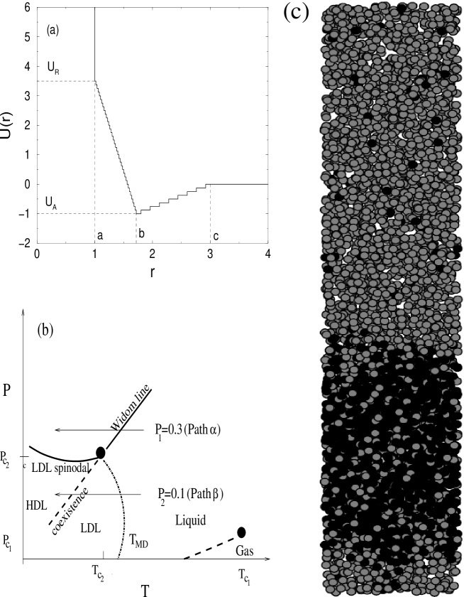
Figure 1: (a) The discretized two-ramp Jagla potential captures much of the essential physics corresponding to the first and the second shells in water. The diameter of the hard core $r_{1}=a$ and the diameter of the soft core $r_{2}=b\approx 1.72$ core determine the two essential length scales corresponding to the first and second shells of water. (b) Schematic P-T phase diagram of the two-ramp Jagla model of plot  1(a). Shown are the two isobaric paths simulated, Path $\alpha~{}(P=P_{1}=0.3>P_{C_{2}})$ and Path $\beta~{}(P=P_{2}=0.1<P_{C_{2}})$. Also shown are the liquid-gas and liquid-liquid critical points (shown as solid circles), the corresponding coexistence lines (dashed lines) and the Widom line (solid line). Also shown is the locus of temperature of maximum density labeled $T_{MD}$ (dotted line). (c) A snapshot of a simulation box for calculation of the Henry constant at $P_{1}=0.3>P_{C_{2}}$ and $T=0.95>T_{C_{2}}$. Black circles represent the hard cores of the Jagla solvent, gray circles represent hard sphere solutes.

In this paper, we attempt to elucidate the connection of the increase of solubility upon cooling with the anomalous thermodynamic properties of pure water. Recently it was shown that the spherically-symmetric Jagla ramp potential (Fig. 1) explains anomalous thermodynamic and dynamic properties of water in terms of the presence of two length scales: a “hard core,” corresponding to the first rigid tetrahedral shell of the nearest neighbors in water, and a wider “soft core,” corresponding to the second (more flexible) shell of neighbors Yan05 ; Xu06b . We will see that the Jagla potential is capable of reproducing the solubility properties of water, and based on this result we will propose a mechanism for the solubility increase of nonpolar compounds in water on cooling.

Using discrete molecular dynamic (DMD) simulations described in Section II, we show in Section III that the solubility of hard sphere solutes in the Jagla solvent has a characteristic minimum as a function of temperature similar to the minimum of the solubility of small nonpolar compounds in water. Hard spheres can be used to describe nonpolar compounds, since the van der Waals interactions among nonpolar compounds are an order of magnitude weaker than the hydrogen bond interactions between water molecules and thus can be neglected in assessing the effect largely caused by the restructuring of hydrogen bonds. In Section IV we relate the solubility increase to the behavior of the excess thermodynamic functions. In Section V, we study the behavior of the beads-on-a-string homopolymer composed of hard sphere monomers immersed in the same Jagla solvent. We show that the radius of gyration $R_{g}$ of the polymer has a sharp minimum as a function of temperature at low constant pressures, indicating that the system may display a LCST at low pressure. At higher pressure, the $R_{g}$ minimum becomes less pronounced, indicating the increase of solubility at intermediate temperatures and decrease of solubility at low temperatures.

II Methods

The interaction potential of the Jagla solvent particles $U(r)$ is characterized by five parameters: the hard core diameter $a$, the soft core diameter $b$, the range of attractive interactions $c$, the depth of the attractive ramp $U_{A}$, and the height of repulsive ramp $U_{R}$ (Fig. 1) Jagla98 , of which three are independent: $b/a$, $c/a$, and $U_{R}/U_{A}$. The most important of these parameters is the ratio of the soft core and hard core diameters, $b/a$, which must be selected close to $r_{2}/r_{1}$, where $r_{1}$ and $r_{2}$ are the positions of the first and the second peaks of the oxygen-oxygen radial distribution function for water. Following Jagla98 ; Xu06b ; Xu05 ; Xu06a we select $b/a=1.72$, $c/a=3$, $U_{R}/U_{A}=3.5$. This choice of parameters produces a phase diagram which qualitatively resembles the water phase diagram with two stable critical points and a wide region of density anomaly bounded by the locus of the temperature of maximum density $T_{\rm MD}$ [Fig. 1(b)]. The slope of the coexistence line between the high density liquid (HDL) and the low density liquid (LDL) in this model is positive—unlike water, for which this slope is negative. In order to use the DMD algorithm Alder59 ; Rapaport78 ; RAPAPORT , we replace the repulsive and attractive ramps with 40 and 8 equal steps, respectively, as described in Xu06b (Fig. 1). We measure length in units of $a$, time in units of $a\sqrt{m/U_{A}}$, where $m$ is the particle mass, density in units of $a^{-3}$, pressure in units of $U_{A}/a^{3}$, and temperature in units of $U_{A}/k_{B}$. This realization of the Jagla model displays a liquid-gas critical point at $T_{c1}=1.446$, $P_{c1}=0.0417$ $\rho_{c1}=0.102$, and a liquid-liquid critical point at $T_{c2}=0.375$, $P_{c2}=0.243$ $\rho_{c2}=0.370$ Xu06b . We model solute particles by hard spheres of diameter $d_{0}$, which we select to be equal to the hard core diameter of the Jagla solvent $d_{0}=a$. The dependence of the solubility on $d_{0}$ is an important question and will be studied elsewhere.

III Calculation of the Henry Constant

We first study the effect of pressure and temperature on the solubility of hard-sphere solutes in the Jagla solvent. In order to do this, we create a system of N=1400 Jagla particles and 2800 hard spheres in a box $L_{x}\times L_{y}\times L_{z}$ with periodic boundaries. We fix $L_{x}=L_{y}=15a$, and vary $L_{z}$ [Fig. 1(c)] to maintain constant pressure and temperature using Berendsen thermostat and barostat. For $T<T_{c1}$, the mixture of Jagla particles and hard spheres segregates and the Jagla particles form a slab of liquid crossing the system perpendicular to the $z$-axis. For each pressure and temperature, we equilibrate the system for 500 time units and measure the mole fraction of hard spheres in the narrow slabs perpendicular to the $z$ axis for another 500 time units. We find that this equilibration time is sufficient if the temperature for the two successive simulations is changed by less then 10%. In each slab we count the numbers $N_{J}$ of Jagla solvent particles and $N_{S}$ of hard sphere solute particles.

We define a slab as a liquid slab if $N_{J}>N_{0}$ and as a vapor slab if $N_{J}\leq N_{0}$, where $N_{0}$ is a temperature and pressure dependent threshold, such that the liquid and vapor slabs form two continuous regions covering the entire system with the exception of a few slabs representing the boundary. To minimize the boundary effects, we exclude from the liquid phase the slabs whose distance to the closest vapor slab is less than $6a$. The analogous criterion is applied to determine the vapor phase. Finally, we find the mole fraction $\Phi=N_{S}/(N_{S}+N_{J})$ of hard spheres in the liquid and vapor phases and compute the Henry constant $k_{H}(T,P)=P\Phi_{v}(T,P)/\Phi_{\ell}(T,P)$, where $\Phi_{v}$ and $\Phi_{\ell}$ are the average mole fractions of hard spheres in the vapor and liquid phases respectively.

Figure 2(a) shows the inverse Henry constant as a function of $T$ for $P=0.1$, $0.2$, and $0.3$. The behavior of the solubility follows the behavior of the inverse Henry constant [Fig. 2(b)], since for $T\ll T_{c_{1}}$ the partial vapor pressure of solvent is very low and, therefore, $P_{v}\approx P$. Hence the solubility $\Phi_{\ell}\approx P/k_{H}(T)$ is inversely proportional to the Henry constant and thus the solubility minimum as function of temperature practically coincides with the maximum of $k_{H}(T)$. One can see that Henry’s law $\partial k_{H}(T,P)/\partial P|_{T}=0$ is approximately correct since $k_{H}(T,P)$ increases by less than 30% when the pressure increases by 200% from 0.1 to 0.3. The most interesting feature of the behavior of the Henry constant is that it has a maximum as function of temperature at $T_{\rm MH}=0.85\pm 0.10$, indicating that the solubility of hard sphere solutes in a Jagla solvent has a minimum at this temperature and increases upon cooling below $T_{\rm MH}$. This behavior is similar to the behavior of the Henry constant of alkanes (C_nH_2n+2) in water, which increases upon cooling below T=$373$K Errington98 . Note that the $T_{\rm MH}$ is much larger than the temperature of maximum density, $T_{\rm MD}=277$K, for both water and for the Jagla model (for which $T_{\rm MD}\approx 0.5$ at $P=0.1$) Xu06b .

IV Relation of the Henry constant to thermodynamic quantities

To relate the behavior of the Henry constant to thermodynamic state functions, we must express the Henry constant in terms of $\Delta g$. At low solute mole fraction $\Phi_{\ell}=y_{\ell}/(x_{\ell}+y_{\ell})$ in the liquid phase, where $x_{\ell}$ and $y_{\ell}$ are the number of moles of solvent and solute respectively, the Gibbs potential $G(x_{\ell},y_{\ell})$ of the solution can be approximated by the first two terms in the Taylor expansion of $G(x_{\ell},y_{\ell})$ around $y_{\ell}=0$ Huang

$$G_{\ell}(x_{\ell},y_{\ell})=x_{\ell}g_{\ell}(0)+y_{\ell}\mu_{\ell}-y_{\ell}T\Delta s_{\rm mix}(\Phi_{\ell}),$$ (3)

where $g_{\ell}(0)$ is the molar Gibbs potential of pure liquid and $\mu_{\ell}$ is the chemical potential of solute in liquid. At low pressures, the analogous approximation can be made for the vapor phase

$$G_{v}(x_{v},y_{v})=x_{v}g_{v}(0)+y_{v}\mu_{v}-y_{v}T\Delta s_{\rm mix}(\Phi_{v}).$$ (4)

Minimization of the sum of the Gibbs potentials of the two phases with respect to $y_{\ell}$ at constant $y\equiv y_{\ell}+y_{v}$ gives the equilibrium condition:

$${\Phi_{v}\over\Phi_{\ell}}=\exp\left({\mu_{\ell}-\mu_{v}\over RT}\right).$$ (5)

The chemical potential of solute in vapor is approximately equal to the molar Gibbs potential of the pure solute. Thus $\mu_{\ell}-\mu_{v}=\Delta g_{0}$, where $\Delta g_{0}=\Delta g+T\Delta s_{\rm mix}$ and $\Delta g$ is given by Eq. (1). If we assume that the vapor is an ideal gas, then $\mu_{v}=\mu_{0}(T)+RT\ln P$, and thus Eq. (5) can be rewritten in the form of the Henry law: $P_{v}/\Phi_{\ell}=k_{H}(T,P)$, where $P_{v}=P\Phi_{v}$ is the partial pressure of solute in vapor and

$$k_{H}(T,P)=P\exp\left({\Delta g_{0}\over RT}\right)$$ (6)

is the Henry constant which in the limit $P\to 0$ does not depend on $P$. Thus the Henry constant has a maximum at the same temperature as $\Delta g_{0}(T)/T$. Since the entropy of mixing does not depend on temperature, this maximum coincides with the maximum of $\Delta g(T)/T$, which as we have seen above corresponds to the temperature at which $\Delta h=0$.

To study the behavior of each thermodynamic term in Eq. (1) at high and low pressures, we compare a mixture of Jagla particles and hard spheres with a given mole fraction $\Phi$ and a given pressure $P$, with a pure solvent and pure solute at the same pressures. We simulate the system at constant $P$ and $\Phi$ in a cubic box with periodic boundaries with given numbers $N_{S}$ and $N_{J}$ of the solute and Jagla particles, respectively, such that $N_{J}+N_{S}=1728$ and $N_{S}/(N_{J}+N_{S})=\Phi$. The systems were simulated at two pressures, $P=P_{1}=0.3>P_{C_{2}}$ [path $\alpha$ of Fig. 1(b)] and $P=P_{2}=0.1<P_{C_{2}}$ [path $\beta$ of Fig. 1(b)]. To find the entropy of the system as function of $T$ and $P$, we change temperature from $T=10$ to $T=0.3$ with a small step and perform thermodynamic integration up to $T=10$ using the first two terms of the virial expansion for $T>10$ with our analytically computed values of the second virial coefficients for hard spheres and Jagla particles. We make sure that the system does not phase segregate at any intermediate temperature.

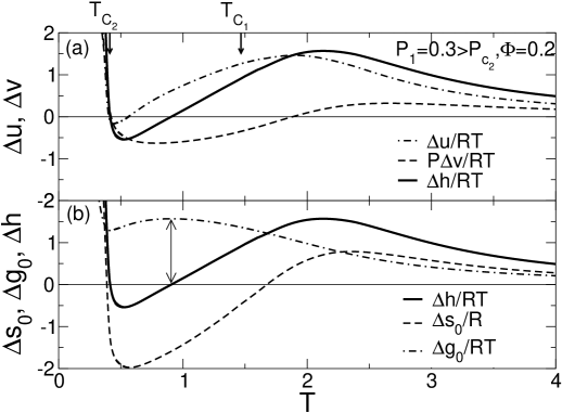
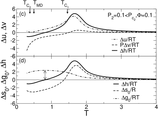
Figure 3: Excess thermodynamic state functions of hard sphere solutes in Jagla liquid solvent computed for (a,b) $P_{1}=0.3>P_{c_{2}}$ and $\Phi=0.2$ and (c,d) for $P_{2}=0.1<P_{c_{2}}$ and $\Phi=0.1$. One can see that the temperature at which $\Delta h=0$ corresponds to the maximum of $\Delta g/RT$ (arrow). Since $P\Delta v$ is only weakly $T$-dependent at high $P$, the decrease of $\Delta h=\Delta u+P\Delta v$ upon cooling for $P=0.3$ is mainly due to the decrease of the potential energy $\Delta u$, while at low pressure, the decrease of $\Delta v$ plays a major role. Note that as the system enters the region of negative thermal expansion coefficient of the pure solvent ($T<T_{\rm MD}$), $\Delta v$ for low $P$ becomes exceedingly negative corresponding to the simple physical picture that as the solvent is cooled, the solvent particles “descend from the repulsive ramp” toward the potential minimum at $r_{2}=b$ so that the average distance between them increases, allowing more space for small solute particles to enter the solvent. At high pressure, both $\Delta u$ and $\Delta v$ become positive at low $T$. This behavior is due to the rapid restructuring of the system as it enters the region of high density liquid above the positively sloped Widom line, which emanates from the critical point located at $T_{c2}=0.375$ and $P_{c2}=0.243$ Xu06a . This behavior leads to the rapid increase of $\Delta g_{0}$ corresponding to the predicted decrease in solubility for $P=0.3$ (Fig. 2). However the calculated solubility in Fig. 2 does not decrease because, at this pressure, the actual solute mole fraction is so large that it is outside the region of applicability of Eq. (6).

Figure 3 shows the behavior of the dimensionless excess state function $\Delta u/RT$, $P\Delta v/RT$, $\Delta h/RT$, $\Delta s_{0}/R$, and $\Delta g_{0}/RT$. One can see that $\Delta h/RT$ becomes negative at the temperature $T_{\rm MH}(\Phi,P)$ of maximal $\Delta g_{0}/RT$ and hence, by Eq. (6), maximal Henry constant. We find $T_{\rm MH}(\Phi=0.2,P=0.3)\approx 0.90$ and $T_{\rm MH}(\Phi=0.1,P=0.1)\approx 0.82$ thus only weakly depending on $\Phi$ and $P$. For both $P$ values, $\Delta v$ becomes negative as the temperature drops below the liquid-gas critical temperature $T_{c_{1}}=1.446$. Since $\Delta u$ decreases with decreasing temperature in this region, $\Delta h$ becomes negative at sufficiently low $T$.

This behavior is consistent with the fact that the solute particles enter relatively large free spaces between the solvent particles which are kept apart not by the hard core but rather by the repulsive ramps, thus creating large negative $\Delta v$ [Figs. 1(b) and 1(c)]. However at high temperatures, the entropic contribution to the free energy is important and the solvent particles in the solute are spread further apart than in the pure sovent. Thus the number of solute particles in the attractive range of the Jagla potential is reduced, leading to $\Delta u>0$. As the temperature decreases, the potential energy of the solution approaches its ground state, which is the same as that of the pure solvent, because the solute particles are small enough to remain in the area unavailable for the solvent particles at low temperatures due to their repulsive ramp interactions [Fig. 1(b)].

At sufficiently low $T$, the excess enthalpy $\Delta h$ of the solution becomes negative, indicating the increase of solubility upon further cooling. Close to $T_{\rm MD}$, the behavior at low and high pressure becomes different. For $P=P_{2}<P_{c2}$ [Fig. 3(b)], the pure solvent starts to expand upon cooling, thus increasing the free space for the solute particles, and further increasing the solubility. This is clearly indicated by the sharp decrease in $\Delta v$. For $P=P_{1}>P_{c2}$ [Fig. 3(a)], there is no $T_{\rm MD}$ and the pure solvent collapses upon crossing the Widom line Xu06a into an HDL-like liquid on the lower side of the Widom line. Thus $\Delta v$ starts to increase upon cooling, and eventually $\Delta v$ becomes positive. On the other hand $\Delta u$ keeps decreasing on decreasing $T$ and becomes negative because the solute particles prevent the solvent particles from “climbing the repulsive ramps” upon compression and therefore help them remain near the minimum of the pair potential.

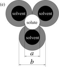
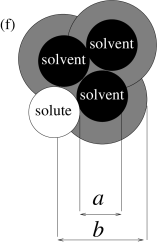
Figure 4: Solvent-solvent correlation function $g_{11}(r)$ computed at $P=0.3$ for pure Jagla solvent, and for the solution with mole fraction $\Phi=0.2$ at (a) $T=0.5$ and (b) $T=0.95$. These plots support the hypothesis that in solution the solvent particles prefer to stay at the soft core distance $r_{2}=b$ and not to “climb the repulsive ramp” occupied by the solute particles. (c) The solvent-solute correlation function $g_{12}$ indicates that the solute particles prefer to stay at the hard core distance $r_{1}=a$ away from the solvent particles. For comparison we plot the correlation function of pure hard spheres at the same temperature $T=0.95$ and pressure $P=0.3$, showing a much smaller peak. (d) The solute-solute correlation functions $g_{22}(r)$ at two different temperatures and the same pressure $P=0.3$ show that at low temperatures the solute particles prefer to stay apart from each other, indicated by the decrease on cooling of the first peak and the increase of the second peak. This effect, that the solute particles clump less at low $T$, is in accord with the increase of solubility upon cooling (cf. Fig. 2). (e) Schematic of the Jagla solvent particles (black) surrounding a hard sphere nonpolar solute (white) of the same diameter $a$. At low $T$ the soft cores (gray) of the solvent particles do not overlap. The distance between the solvent particles corresponds to the potential energy minimum $r_{1}=b$ in Fig. 1(a), thus the solvent particles form a cage around the hard sphere nonpolar solutes.(f) Schematic of the same situation but now for $T\approx T_{MH}$, the temperature of maximum Henry constant and hence minimum solubility.

To test this explanation directly, we compute for $P=0.3$ and $T=0.5$ the solvent-solvent density correlation function, $g_{11}(r)$, in the pure solvent and in the solution with solute mole fraction $\Phi=0.2$, [Fig. 4(a)]. We see that the first peak in $g_{11}(r)$, corresponding to the solvent particles staying at the hard core distance in the pure solvent, significantly decreases in the solution. In contrast, the second peak, corresponding to the solvent particles staying at the soft core distance, increases. The behavior of the cross-correlation function $g_{12}(r)$ of the solute and solvent [Fig. 4(c)] indicates that indeed the solute particles prefer to remain very close to the solvent particles in the region unavailable for solvent particles due to their repulsive ramp interactions. The behavior of the solute-solute correlation function $g_{22}(r)$ indicates a small decrease in the first peak and an increase in the second peak upon cooling [Fig. 4(d)], corresponding to the increase of solubility. Overall, the structure of the solution is more pronounced than in the pure solvent case, indicated by negative $\Delta s_{0}$ [Fig. 3(b)].

This behavior of the Jagla solvent with hard sphere solutes is analogous to the behavior of water molecules in the presence of nonpolar compounds. The hard core of the Jagla model corresponds to the rigid tetrahedron (first shell) of water molecules linked by hydrogen bonds to a central molecule. A particle at the hard core distance in the Jagla model corresponds to an extra (fifth) water molecule entering the first shell. This molecule may cause the formation of a bifurcated hydrogen bond Sciortino of higher potential energy than the normal hydrogen bond. The nonpolar solute molecules in water remain close to the first shell of water molecules, and thus prevent extra water molecules entering into the first shell and forming bifurcated hydrogen bonds. Thus in water, solute particles help stabilize hydrogen bonds. The second shell of water becomes more structured by forming cages around the solute molecules without breaking any hydrogen bonds.

For $P=P_{2}<P_{c_{2}}$, the $g_{11}(r)$ for pure solvent and solution are practically indistinguishable (not shown), with only slight decrease of the overall number of solvent particles within the attractive range in the solution compared to the pure solvent, corresponding to small $\Delta u>0$. The behaviors of $g_{12}(r)$ and $g_{22}(r)$ at low pressures (not shown) are practically the same as at high pressures. This means that for low pressures the increase of the solubility upon cooling is mainly because of the decrease of $\Delta v$ due to the small and even negative thermal expansion coefficient of the pure solvent. We expect that the relative strength of the two contributions, energetic and volumetric, to $\Delta h$ strongly depends on the size of the solute particles. Accordingly, in water one might expect both mechanisms to be present, depending on $P$, and on the nature of the solute.

To check the validity of our calculations of the Henry constant $k_{\rm H}$ and the thermodynamic excess quantities, we compare $k_{\rm H}$ obtained directly by measuring the mole fraction of hard spheres in the slabs of Sec. III with $k_{\rm H}$ computed using Eq. (6). Figure 2 shows that although the individual contributions of different terms to $\Delta g$ behave in a complex way, the resulting behavior of the Henry constant is in good agreement with the direct simulations near the solubility minimum. Note the failure of thermodynamic predictions at high and low temperatures. The dramatic solubility drop predicted by Eq. (6) at $P=0.3$ is because at fixed mole fraction, the amount of solute particles become insufficient to prevent the solute from collapse, and eventually $\Delta u$ also starts to increase upon cooling making $\Delta h>0$ at low temperatures. This predicted decrease of the solubility upon cooling is not observed in the direct simulations (Fig. 2). The discrepancy between the thermodynamic predictions and actual behavior of the Henry constant is due to the fact that at low temperatures the mole fraction $\Phi_{\ell}>0.3$ is so high, that the linear Taylor expansion of Eq. (3) is no longer valid. Thus, in reality, there are still enough solute particles to prevent the solution from collapsing into an HDL-like liquid. In the next section, concerning polymer solution, we observe the decrease of solvent quality upon cooling at $P>P_{c_{2}}$ because the polymer monomers do not have sufficient local mole fraction to keep the solution from collapse.

V Polymer swelling upon cooling

In order to relate the maximum of solubility of nonpolar compounds to the polymer LCST and protein denaturation, we next study the behavior of a polymer composed of $M=44$ monomers modeled by hard spheres of diameter $d_{0}=a$. We model covalent bonds by linking the hard spheres with the potential

$$U_{\rm bond}(r)=\left\{\begin{array}[]{ll}\infty&r<d_{1}\\ 0&d_{1}<r<d_{2}\\ \infty&r>d_{2}\end{array}\right.,$$ (7)

where the minimal extent of the bond is $d_{1}=a$ and the maximal extent is $d_{2}=1.2a$. We simulate for $t_{m}$ time units the trajectory of the polymer at constant $T$ and $P$ in a cubic box containing $N=1728$ Jagla solvent particles with periodic boundaries. We calculate the polymer radius of gyration $R_{g}(t_{k})$, where

$$R_{g}^{2}(t_{k})\equiv{M\sum_{i=1}^{M}(x_{i}^{2}+y_{i}^{2}+z_{i}^{2})-\left(\sum_{i=1}^{M}x_{i}\right)^{2}-\left(\sum_{i=1}^{M}x_{i}\right)^{2}-\left(\sum_{i=1}^{M}x_{i}\right)^{2}\over M^{2}}$$ (8)

at equidistant times $t_{k}\equiv k\Delta t$, where $\Delta t\equiv 1$, and we calculate the rms radius of gyration $R_{g}$, where $R_{g}^{2}\equiv\sum_{k=1}^{m}R_{g}^{2}(t_{k})/m$, and $m\equiv t_{m}/\Delta t$.

Figure 5 shows the behavior of the radius of gyration of a polymer as a function of temperature for six values of pressure. Also shown for the $P=0.02$ case is the inverse Henry constant. One can see that for small pressures, $R_{g}$ reaches a deep minimum at $T=T_{\rm MR}(P)$, which occurs above the maximum of the Henry constant $T=T_{\rm MH}(P)$. As pressure increases, the minimum becomes less pronounced and $T_{\rm MR}(P)$ shifts to higher temperatures and eventually, at $P=0.4$, almost disappears. According to the de Gennes-Flory-Huggins theory Rubinstein03 , the radius of gyration is a function of polymer length and the solvent quality $\chi$:

$$R_{g}=\ell N^{1/2}f(z),$$ (9)

where $z=(2\chi-1)N^{1/2}$ and

$$f(z)\sim\left\{\begin{array}[]{ll}|z|^{-1/3}&z\ll 0\\ 1&z=0,\\ z^{2\nu-1}&z>0\end{array}\right.,$$ (10)

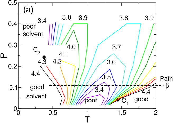
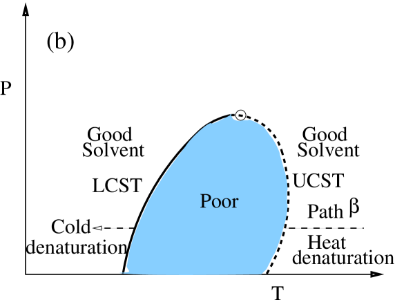
Figure 6: (a) Contours of equal $R_{g}$ in the P-T plane, showing regions of good and poor solvent; the numbers denote the value of $R_{g}$. The filled circles $C_{1}$ and $C_{2}$ indicate the liquid-gas and liquid-liquid critical points. Note that at low $P$, on decreasing $T$ along path $\beta$, one passes from a region of good solvent (swollen “denatured” polymers) to a region of poor solvent (collapsed polymers) and finally to a region of good solvent (“cold denaturation”). (b) Schematic illustration of the loci of the lower critical solution temperature (LCST) and the upper critical solution temperature (UCST) for a polymer chain such as studied here. The UCST delineates the region of high-$T$ swelling (“heat denaturation of a protein”) while LCST delineates the region of low-$T$ swelling (“cold denaturation of a protein”) sampled by path $\beta$.

where $\nu\approx 0.588$ is the Flory exponent for $R_{g}$. Values of $\chi<1/2$ correspond to a “poor” solvent, in which the polymer chain is collapsed and $R_{g}\sim N^{1/3}$. Values of $\chi>1/2$ correspond to a “good” solvent where the polymer swells and $R_{g}\sim N^{\nu}$. The value $\chi=1/2$ corresponds to the “theta condition” with $R_{g}\sim N^{1/2}$. Thus for a polymer of a given length, the radius of gyration monotonically increases with solvent quality and can be used to calculate lines of the equal solvent quality in the $P-T$ plane. We tested numerically that near the minimum of $R_{g}$ for $P\leq 0.2$, $R_{g}\sim N^{1/3}$, so the solvent quality is poor. For $T\leq 0.5$, $R_{g}$ is comparable with $R_{gv}=4.77$ in a vacuum, and hence the solvent quality is good. Thus the theta condition corresponds to some temperature between $T=0.5$ and the value of $T$ at which $R_{g}$ has a minimum. Accordingly, the LCST which differs from the theta point by a term of the order of $1/\sqrt{M}$ Rubinstein03 is also located in this region. Assuming that $R_{g}=3.5$ for $N=44$ corresponds to the theta point, we construct a region in the $P-T$ plane of approximate location of the LCST which merges with the upper critical solution temperature (UCST) at $P=0.12$ and $T=1.25$ (Fig. 6). The region of the $P-T$ plane below this line corresponds to the poor solvent in which sufficiently long polymer chains segregate from the sufficiently concentrated solution. This region lies below $P_{c_{2}}$ and significantly above the $T_{\rm MD}$ line in the $P-T$ plane. On the high temperature side, the region where $R_{g}<3.5$ is bounded by the liquid-gas critical point.

Since the driving force of the folding of globular proteins is the formation of the hydrophobic core, one can imagine that the regions in the $P-T$ plane in which the various proteins can fold into their native states must have similar shapes.

VI Discussion and Conclusions

Our work suggests a physical mechanism for the increase of solubility of nonpolar solvents upon cooling (Fig. 2) connecting the cold denaturation of a polymer to the LCST. These phenomena are related to thermodynamic anomalies of pure water because both thermodynamic and solubility properties are reproduced in the simple Jagla solvent model. Both of these are caused by the existence of two repulsive scales in the effective model potential, the hard core corresponding to the first tetrahedral shell of water molecules and the soft core corresponding to the second shell of water molecules. However, the temperature range in which cold denaturation and the solubility minimum occur does not directly coincide with the regions of other water anomalies, which are generally placed at lower temperatures.

Interestingly, the region of poor solvent, corresponding to the sharp minimum in $R_{g}$ lies below the critical pressure of the second critical point. Above this pressure, the behavior of the solvent quality changes, being almost constant in the wide range of temperatures much above $T_{c2}$, but dramatically decreasing as we approach $T_{c2}$, indicating that the HDL in the Jagla model is a poor solvent, while the LDL is a good solvent. This behavior is in accord with the thermodynamic studies of Section IV where a sharp increase in $\Delta g$ upon cooling near the Widom line is found. The physical reason for this is that LDL in the Jagla model has a larger free volume for the hard spheres to enter and is also less ordered than HDL, so entering of the hard spheres does not destroy this order. Whether this situation for water is the same as or the opposite is not clear, since LDL in water, although having larger volume, is more ordered than HDL. New simulations, underway, involving water models that have a liquid-liquid critical point in the accessible region and a chain of Lennard-Jones monomers may answer this question.

Acknowledgments

We thank C. A. Angell, P. G. Debenedetti, M. Marqués, P. J. Rossky, S. Sastry, and Z. Yan for helpful discussions, the Office of Academic Affairs of Yeshiva University for sponsoring the high performance cluster, and NSF for financial support.

Figure 2: (a) Symbols indicate our simulation results of the inverse Henry constant of hard sphere solutes in the Jagla liquid solvent for three different pressures. Lines indicate our theoretical predictions based on calculations of excess thermodynamic state functions—see Eq. (6) and Fig. 3. Note the failure of the theoretical predictions for both high and low temperatures in the $P=0.3$ case caused by the fact that Eq. (6) is valid only in the limit of small liquid mole fraction $\Phi_{\ell}$ of solute in liquid. (b) The solubility of the hard sphere solutes in the Jagla solvent as function of temperature. The solubility minimum roughly coincides with the minimum of the inverse Henry constant.

Figure 5: Dependence on temperature of the average radius of gyration of $M=44$ polymer comprising $M=44$ hard sphere monomers for different pressures. The dashed vertical lines show $T_{\rm MH}(P)$ of the maximum of the Henry constant. We also show that for the lowest pressures the solubility minimum of the hard sphere solute particles roughly coincides with the $R_{g}$ minimum. We find the rms radius of gyration in a vacuum is $R_{gv}=4.77$. The evolution of the polymer chain in the solvent is much slower than in a vacuum, so to calculate a reliable $R_{g}$, we must carefully estimate the error bars. In order to do so we divide the entire set of $m$ measurements into $m/n$ equal groups of $n\leq m/2$ subsequent values $R_{g}^{2}(t_{k})$, and find the average for each group $\langle R_{g}^{2}\rangle_{i}$, $i=1,2,...,m/n$ and the standard deviation $\sigma_{n}$ of $\langle R_{g}^{2}\rangle_{i}$. If the values $\langle R_{g}^{2}\rangle_{i}$ were independent, the error bars on their average could be determined as $\sigma_{n}/\sqrt{m/n-1}$, and this estimate would not depend on $n$. In fact, for small $n$, $\sigma_{n}/\sqrt{m/n-1}$ is an increasing function of $n$, which reaches the plateau at $n=\tau/\Delta t$, where $\tau$ is the correlation time. Accordingly, we determine the error bar as $\max_{n}[\sigma_{n}/\sqrt{m/n-1}]$, checking that this quantity indeed reaches a plateau for a given number of observations $m$. If this quantity does not reach the plateau, it means that the time of averaging is insufficient and we must increase $m$.

References

- (1) S. S. Zumdahl, Chemistry, 4th Edition (Houghton Mifflin, Boston, 1997).
- (2) W. E. Acree Jr, Thermodynamic Properties of Nonelectrolyte solutions (Academic Press, Orlando, 1984).
- (3) O. Konrad and T. Lankau, J. Phys. Chem. B 109, 23596 (2005).
- (4) P. J. Lenart and A. Z. Panagiotopoulos, J. Phys. Chem. B 110, 17200 (2006).
- (5) P. E. Krouskop, A. Geiger, D. Paschek, and A. Krukau, J. Chem. Phys.124, 016102 (2006).
- (6) P. J. Flory, R. A. Orwoll, and A. Virj, J. Amer. Chem. Soc. 86, 3507 (1964).
- (7) P. J. Flory, J. Amer. Chem. Soc. 87, 1833 (1965).
- (8) I. Prigogine, The Molecular Theory of Solutions (North Holland, Amsterdam, 1957).
- (9) H. T. Van and D. Patterson, J. Solution Chem. 11, 793 (1984).
- (10) M. Costas and D. Patterson, J. Solution Chem. 11, 807 (1984).
- (11) D. Patterson and G. Delmas, Discussions Faraday Soc. 49, 98 (1970).
- (12) P. Paricaud, A. Galindo, and G. Jackson, Molecular Physics, 101, 2575 (2003).
- (13) C. N. Pace and Ch. Tanford, Biochemistry 7, 198 (1968).
- (14) P. L. Privalov and S. J. Gill, Adv. Protein Chem. 39, 191 (1988).
- (15) P. L. Privalov, Crit. Rev. Biochem. Mol. Biol. 25, 281 (1990).
- (16) J. Jonas, ACS Symp. S 676, 310 (1997).
- (17) D. Paschek, S. Nonn, and A. Geiger, Phys. Chem. Chem. Phys. 7. 2780 (2005).
- (18) M. I. Marqués, Physica Status Solidi. A 203, 1487 (2006).
- (19) M. S. Moghaddam, S. Shimizu, and H. S. Chan, J. Amer. Chem. Soc. 127, 303 (2005).
- (20) D. Pascheck, J. Chem. Phys. 120, 10605 (2004).
- (21) H. S. Frank and M. W. Evans, J. Chem. Phys. 13 507 (1945).
- (22) A. K. Soper, L. Dougan, J. Crain, and J. L. Finney, J. Phys. Chem. B 110, 3472 (2006).
- (23) J. R. Errington, G. C. Boulougouris, I. G. Economou, A. Z. Panagiotopoulos, and D. N. Theodorou, J. Phys. Chem. B 102, 8865 (1998).
- (24) Z. Yan, S. V. Buldyrev, N. Giovambattista, and H. E. Stanley, Phys. Rev. Lett. 95 130604 (2005).
- (25) L. Xu, S. V. Buldyrev, C. A. Angell, and H. E. Stanley, Phys. Rev. E 74, 031108 (2006)
- (26) E. A. Jagla, Phys. Rev. E 58, 1478 (1998).
- (27) L. Xu, P. Kumar, S. V. Buldyrev, S.-H. Chen, P. H. Poole, F. Sciortino, and H. E. Stanley, Proc. Natl. Acad. Sci. 102, 16558 (2005).
- (28) L. Xu, I. Enrenberg, S. V. Buldyrev, and H. E. Stanley, J. Phys.-Condens. Matt. 18, S2239 (2006).
- (29) B. J. Alder and T. E. Wainwright, J. Chem. Phys. 31, 459 (1959).
- (30) D. C. Rapaport, J. Phys. A 11, L213 (1978).
- (31) D. C. Rapaport, The Art of Molecular Dynamics Simulation (Cambridge University Press, Cambridge, 1997).
- (32) K. Huang, Statistical Mechanics, 2nd Edition (John Wiley & Sons, New York, 2000).
- (33) F. Sciortino, A. Geiger, and H. E. Stanley, Phys. Rev. Lett. 65, 3452 (1990); Nature (London) 354, 218 (1991); J. Chem. Phys. 96, 3857 (1992).
- (34) M. Rubinstein and R. H. Colby, Polymer Physics (Oxford University Press, Oxford, 2003).