Projected single-spin flip dynamics in the Ising Model

Abstract

We study transition matrices for projected dynamics in the energy-magnetization space, magnetization space and energy space. Several single spin flip dynamics are considered such as the Glauber and Metropolis canonical ensemble dynamics and the Metropolis dynamics for three multicanonical ensembles: the flat energy-magnetization histogram, the flat energy histogram and the flat magnetization histogram. From the numerical diagonalization of the matrices for the projected dynamics we obtain the sub-dominant eigenvalue and the largest relaxation times for systems of varying size. Although, the projected dynamics is an approximation to the full state space dynamics comparison with some available results, obtained by other authors, shows that projection in the magnetization space is a reasonably accurate method to study the scaling of relaxation times with system size. The transition matrices for arbitrary single-spin flip dynamics are obtained from a single Monte-Carlo estimate of the infinite temperature transition-matrix, for each system size, which makes the method an efficient tool to evaluate the relative performance of any arbitrary local spin-flip dynamics. We also present new results for appropriately defined average tunnelling times of magnetization and compute their finite-size scaling exponents that we compare with results of energy tunnelling exponents available for the flat energy histogram multicanonical ensemble.

I Introduction

The dynamical critical behavior of statistical physics models is a problem that attracts considerable attentionHH77 ; Sokal97 ; Nightingale96 ; Nightingale00 . From a fundamental point of view one is interested in the identification and characterization of the different dynamical universality classes, known to be more restricted than the static ones. Different algorithms for canonical ensemble simulations have been proposed belonging to different universality classescluster ; Wolff89 . Still, increasing relaxation times with system size are a major limitation to the statistical precision of the numerical estimates obtained in the simulations. New algorithms, aiming to estimate the number of states of a given energy, have also been proposedmulticanonical ; lee93 ; bhanot . These algorithms simulate a multicanonical ensemble with the advantage that a single simulation provides information on the properties of the system in a wide temperature range. However, such algorithms also suffer from slowing down with increasing system size and the study of their dynamical properties with simple and efficient methods is essential to ascertain their relative performance.

Many numerical methods have been used to study stochastic dynamics of statistical physics models. These methods measure the largest relaxation time of the dynamics, a time which increases with system size according to dynamic finite-size scaling theory. The exact diagonalization of the transition matrix in the full state space can be done only for very small systems. To overcome this limitation, one can instead estimate by Monte-Carlo methods the auto-correlation function of the slowest observable in the system, that whose long time behavior gives the largest relaxation time. Although this method is free of systematic errors, one needs to consider very long simulation runs to get a reasonably small statistical error in the auto-correlation function. Several other methods have been used, including a variational techniqueNightingale96 ; Nightingale00 allowing the estimation of the sub-dominant eigenvalue of the full state-space transition matrix.

Projected dynamics was proposed to study metastability and nucleation in the Ising modelLee95 ; Shteto97 ; Shteto99 ; Kolesik97 ; Kolesik98 ; Novotny01 . The idea behind this method is to derive a dynamics in a restricted space of one or several variables. Choosing appropriately such variables and neglecting non-Markovian memory terms one hopes that the resulting approximated Markovian dynamics is a good approximation to the full state space dynamics. The usefulness of the method has been proved in the context of the study of metastability in the Ising model where the direct dynamic Monte-Carlo simulation is unable to bare with the large time-scale of the problemNovotny01 . The non-lumpability of the the full state-space transition rate matrix with respect to energy and magnetization classification of the states leads to the upcoming of memory terms when projecting the dynamics in these restricted spacesKemeny76 ; Novotny01 . To recover the Markovian character of the dynamics, these memory terms are neglected and the resulting projected dynamics becomes only approximated.

In this article we study the projected dynamics behavior for the square lattice, nearest-neighbor, Ising model, in the energy and magnetization spaces for two local spin flip algorithms. Namely, the Glauber and the Metropolis et al.MetGl critical canonical ensemble dynamics, and three multicanonical algorithms: the flat energy-magnetization histogram, the flat energy histogram and the flat magnetization histogram dynamics. Although the dynamics associated with the transition rate matrices in these restricted spaces are only approximate, we show, by comparison with full state space results, that they can be used to get reasonably accurate estimates of the dynamical properties. From the numerical diagonalization of these matrices, and the determination of their sub-dominant eigenvalue, we compute the largest relaxation times for systems of varying size. The method proposed can be applied to other models and other dynamics thus leading to a simple and efficient estimation of the scaling with system size of the largest relaxation time. Such studies are needed to assess the relative performance of Monte-Carlo simulation algorithms.

Projected dynamics transition rate matrices were also considered in the context of the transition matrix Monte-CarloWang99 ; Wang01 . Using an acceptance probability written in terms of the infinite temperature energy space transition matrix it is possible to perform simulations that visit with equal probability the spectra of energies of the model thus doing flat energy histogram simulations. For the case of the Ising model that we consider in this work this algorithm is easily generalized to simulations with a flat energy and magnetization histogram. We use this flat energy-magnetization histogram ensemble to numerically estimate the infinite temperature transition rate matrix in the space of energy and magnetization from which all the results presented in this work were derived.

For multicanonical algorithms, average tunnelling times between the ground-state and states with higher energy (for example zero energy) have been considereddayal2004 . It has been shown that these tunnelling times may scale differently with system size when we consider going up (from a low energy to a high energy) or going down in the energycosta2005 . We present new results for average tunnelling times of magnetization, in several multicanonical ensembles, using projected dynamics, that show a similar behavior and that can be compared with results of other authors for tunnelling times in the energy space.

The new method proposed by us, to study approximately the local dynamics, is efficient because: (1) the dynamic exponents estimates are reasonably accurate when compared with corresponding quantities obtained by other methods; (2) any, arbitrary, single-spin flip dynamics can be studied from a single Monte-Carlo estimation of an infinite temperature transition matrix in the energy-magnetization space (corresponding to acceptance of all the proposed configurations); the consideration of a specific dynamics comes only from the weighting of this matrix with the corresponding acceptance probability; (3) the dimensional reduction achieved by the projection allows the application of matrix diagonalization techniques for bigger system sizes.

The outline of the paper is as follows: In section II we discuss the projection procedure, in section III we show how the infinite temperature transition matrix is computed from Monte-Carlo simulations for different system sizes and we define the projected transition matrices for the different ensembles and dynamics considered, in section IV we present results for the largest relaxation times and the corresponding dynamical exponents, in section V we define and compute tunnelling times in the magnetization space and their finite-size scaling exponents and, finally, in section VI we summarize our main conclusions.

II Projected dynamics

The Markov chain master equation in the full state space is:

$$\frac{dP(\vec{\sigma},t)}{dt}=\sum_{\vec{\sigma}^{\prime}}[W(\vec{\sigma},\vec{\sigma}^{\prime})P(\vec{\sigma}^{\prime},t)-P(\vec{\sigma},t)W(\vec{\sigma}^{\prime},\vec{\sigma})],$$ (1)

where $\vec{\sigma}$ denotes a state of the system, $P(\vec{\sigma},t)$ is the probability for the system to be in a given state at time $t$ and $W(\vec{\sigma},\vec{\sigma}^{\prime})$ is the transition rate from state $\vec{\sigma}^{\prime}$ to $\vec{\sigma}$. In the case of an Ising model $\vec{\sigma}\equiv(\sigma_{1},...,\sigma_{N})$ specifies the state of each of $N$ spins of the system, $\sigma_{i}$, that can take two values, $\sigma_{i}=\pm 1$. The transition rate obeys detailed balance

$$P_{st}(\vec{\sigma})W(\vec{\sigma}^{\prime},\vec{\sigma})=P_{st}(\vec{\sigma}^{\prime})W(\vec{\sigma},\vec{\sigma}^{\prime})$$ (2)

relatively to a stationary distribution, $P_{st}(\vec{\sigma})$, which we consider to be an arbitrary function $P_{st}(E(\vec{\sigma}),M(\vec{\sigma}))$, of the energy $E(\vec{\sigma})=-\sum_{\langle i,j\rangle}\sigma_{i}\sigma_{j}$ (where the sum is over all neighbor pairs, $\langle i,j\rangle$), and the magnetization $M(\vec{\sigma})=\sum_{i}\sigma_{i}$.

The detailed balance equation can be summed up relative to all $\vec{\sigma}$ states with a given energy $E=E(\vec{\sigma})$ and magnetization $M=M(\vec{\sigma})$, and all $\vec{\sigma}^{\prime}$ states with energy $E^{\prime}=E(\vec{\sigma}^{\prime})$ and magnetization $M^{\prime}=M(\vec{\sigma}^{\prime})$, to obtain:

$$\sum_{\vec{\sigma},\vec{\sigma}^{\prime}}P_{st}(\vec{\sigma})W(\vec{\sigma}^{\prime},\vec{\sigma})\delta_{E,E(\vec{\sigma})}\delta_{E^{\prime},E(\vec{\sigma}^{\prime})}\delta_{M,M(\vec{\sigma})}\delta_{M^{\prime},M(\vec{\sigma}^{\prime})} =$$ (3)

$$\sum_{\vec{\sigma},\vec{\sigma}^{\prime}}P_{st}(\vec{\sigma}^{\prime})W(\vec{\sigma},\vec{\sigma}^{\prime})\delta_{E,E(\vec{\sigma})} \delta_{E^{\prime},E(\vec{\sigma}^{\prime})} \delta_{M,M(\vec{\sigma})}\delta_{M^{\prime},M(\vec{\sigma}^{\prime})}$$

being $\delta_{a,b}$ the Kronecker delta. Since the stationary distribution is assumed to be a function of the energy and magnetization only, it can be taken out of the summation, giving

$$p(E,M)T(E^{\prime},M^{\prime};E,M)=p(E^{\prime},M^{\prime})T(E,M;E^{\prime},M^{\prime})$$ (4)

where $p(E,M)=P_{st}(E,M)\Omega(E,M)$ is the stationary probability for the system to have energy $E$ and magnetization $M$, and $\Omega(E,M)$ is the number of states with energy $E$ and magnetization $M$. In this expression, we have defined,

$$T(E^{\prime},M^{\prime};E,M)=\frac{1}{\Omega(E,M)}\sum_{\vec{\sigma},\vec{\sigma}^{\prime}}W(\vec{\sigma}^{\prime},\vec{\sigma})\delta_{E,E(\vec{\sigma})}\delta_{E^{\prime},E(\vec{\sigma}^{\prime})}\delta_{M,M(\vec{\sigma})}\delta_{M^{\prime},M(\vec{\sigma}^{\prime})}$$ (5)

as the transition matrix between energy and magnetization states $(E,M)$ and $(E^{\prime},M^{\prime})$.

Summing up the master equation in the same way we would obtain the evolution equation for the time dependent probability $p(E,M,t)$ for the system to have energy $E$ and magnetization $M$ at time $t$:

$$\frac{dp(E,M,t)}{dt}=\sum_{E^{\prime},M^{\prime}}[T(E,M;E^{\prime},M^{\prime};t)p(E^{\prime},M^{\prime},t)-p(E,M,t)T(E^{\prime},M^{\prime};E,M;t)],$$ (6)

with a time-dependent transition matrix:

$$T(E^{\prime},M^{\prime};E,M;t)=\frac{1}{p(E,M,t)}\sum_{\vec{\sigma},\vec{\sigma}^{\prime}}P(\vec{\sigma},t)W(\vec{\sigma}^{\prime},\vec{\sigma})\delta_{E,E(\vec{\sigma})}\delta_{E^{\prime},E(\vec{\sigma}^{\prime})}\delta_{M,M(\vec{\sigma})}\delta_{M^{\prime},M(\vec{\sigma}^{\prime})}$$ (7)

This time dependent matrix approaches the transition rate matrix in Eq. (5) for large times when $P(\vec{\sigma},t)/p(E,M,t)\rightarrow 1/\Omega(E,M)$. The so-called projected dynamics neglects this time dependence and considers instead the Markov process associated with $T(E^{\prime},M^{\prime};E,M)$:

$$\frac{dp(E,M,t)}{dt}=\sum_{E^{\prime},M^{\prime}}[T(E,M;E^{\prime},M^{\prime})p(E^{\prime},M^{\prime},t)-p(E,M,t)T(E^{\prime},M^{\prime};E,M)].$$ (8)

Starting with the projection operator technique, in a discrete time formulation, the approximation can be regarded as equivalent to dropping out some memory termsShteto99 . Note that the dynamics of the Markovian process associated with these transition matrices would be equivalent to the full state space dynamics if it were lumpableKemeny76 with respect to a classification of the states in terms of energy and magnetization. However, this is known not to be the case for canonical ensemble dynamicsNovotny01 , although the flat magnetization ensemble that we study later is lumpable with respect to a magnetization classification of the states.

Further projection on the energy space can be done by summing for all $M$ and $M^{\prime}$ the detailed balance condition in the $E,M$ space (Eq.4) :

$$p(E)\sum_{M,M^{\prime}}\frac{p(E,M)}{p(E)}T(E^{\prime},M^{\prime};E,M)=p(E^{\prime})\sum_{M,M^{\prime}}\frac{p(E^{\prime},M^{\prime})}{p(E^{\prime})},T(E,M;E^{\prime},M^{\prime})$$ (9)

which is a detailed balance relation $p(E)T(E^{\prime},E)=p(E^{\prime})T(E,E^{\prime})$ in the energy space with a projected transition matrix

$$T(E^{\prime};E)=\sum_{M,M^{\prime}}\frac{p(E,M)}{p(E)}T(E^{\prime},M^{\prime};E,M).$$ (10)

Note that for the ensembles where $P_{st}(\vec{\sigma})$ depends just on the energy (and not on the magnetization) the previous expression can be simplified to:

$$T(E^{\prime};E)=\frac{1}{\Omega(E)}\sum_{M,M^{\prime}}\Omega(E,M)T(E^{\prime},M^{\prime};E,M)=\frac{1}{\Omega(E)}\sum_{\vec{\sigma},\vec{\sigma}^{\prime}}W(\vec{\sigma}^{\prime},\vec{\sigma})\delta_{E,E(\vec{\sigma})}\delta_{E^{\prime},E(\vec{\sigma}^{\prime})}$$ (11)

with $\Omega(E)=\sum_{M}\Omega(E,M)$ is the number of states with energy $E$. If $P_{st}(\vec{\sigma})$ depends on energy and magnetization simultaneously the above simplification can not be done.

The transition matrix $T(E,E^{\prime})$ can be used to define a Markov chain dynamics in the restricted energy space:

$$\frac{dp(E,t)}{dt}=\sum_{E^{\prime}}[T(E;E^{\prime})p(E^{\prime},t)-p(E,t)T(E^{\prime};E)].$$ (12)

In the same way we can obtain a detailed balance relation in the magnetization space:

$$p(M)\sum_{E,E^{\prime}}\frac{p(E,M)}{p(M)}T(E^{\prime},M^{\prime};E,M)=p(M^{\prime})\sum_{E,E^{\prime}}\frac{p(E^{\prime},M^{\prime})}{p(M^{\prime})}T(E,M;E^{\prime},M^{\prime}),$$ (13)

which is a detailed balance relation $p(M)T(M^{\prime},M)=p(M^{\prime})T(M,M^{\prime})$ in the magnetization space with a projected transition matrix

$$T(M^{\prime};M)=\sum_{E,E^{\prime}}\frac{p(E,M)}{p(M)}T(E^{\prime},M^{\prime};E,M).$$ (14)

The transition matrix $T(M,M^{\prime})$ can be used to define a Markov chain dynamics in the restricted magnetization space:

$$\frac{dp(M,t)}{dt}=\sum_{M^{\prime}}[T(M;M^{\prime})p(M^{\prime},t)-p(M,t)T(M^{\prime};M)].$$ (15)

Nevertheless the approximation assumed in the projected dynamics, the detailed balance relations satisfied by the transition matrices defined above assure that the long time behavior of the related stochastic processeses defined by Eqs. (8), (12) and (15) are still characterized by the correct stationary probability distributions $p(E,M)$, $p(E)$ and $p(M)$, respectively.

In the following sections, we study single spin flip dynamics in the canonical ensemble characterized by the stationary distribution at inverse temperature $\beta$, $P_{st}(\vec{\sigma})=\exp(-\beta E(\vec{\sigma}))/Z$ as well as three multicanonical ensembles with flat energy-magnetization, flat energy and flat magnetization histograms with $P_{st}(\vec{\sigma})=1/\Omega(E,M)$, $P_{st}(\vec{\sigma})=1/\Omega(E)$ and $P_{st}(\vec{\sigma})=1/\Omega(M)$, respectively. Note that $\Omega(M)=\sum_{E}\Omega(E,M)$ is exactly known to be $\Omega(M)=\binom{N}{\frac{N+M}{2}}$ and that an efficient numerical scheme (not used by us in the present work) developed by Beale Beale96 allows to compute exactly $\Omega(E)$ for the two-dimensional Ising model for moderate system sizes $N$.

III Numerical calculation of transition matrices

We now explain our method to compute numerically the transition matrices $T(E^{\prime},M^{\prime};E,M)$, $T(E^{\prime},E)$ and $T(M^{\prime},M)$ defined in Eqs. (5), (10) and (14), respectively. We start by recalling that for single spin flip dynamics the transition rate $W(\vec{\sigma}^{\prime},\vec{\sigma})$ can be separated in a proposal step and an acceptance step. In the proposal step we choose, with equal probability, one of the spins of the system and propose to flip it. Thus a given system state may have a non-zero transition rate to $N$ other system states that differ in the state of a single spin. In the acceptance step we accept the proposed configuration with a probability $a(E^{\prime},M^{\prime};E,M)$ that we assume depends only on the energy and magnetization of the initial and final configurations.

Consider the detailed balance relation (4) when we accept all the proposed configurations. This is the case, for example, in the Metropolis et al. algorithm at infinite temperature. The probability to measure an energy $E$ and magnetization $M$ is then equal to $\Omega(E,M)/2^{N}$ since all states have equal probability. Thus we can write the relation,

$$\Omega(E,M)T_{\infty}(E^{\prime},M^{\prime};E,M)=\Omega(E^{\prime},M^{\prime})T_{\infty}(E,M;E^{\prime},M^{\prime})$$ (16)

known as the broad histogram equationbhm . For a general single spin flip algorithm characterized by $a(E^{\prime},M^{\prime};E,M)$we can write,

$$T(E^{\prime},M^{\prime};E,M)=T_{\infty}(E^{\prime},M^{\prime};E,M)a(E^{\prime},M^{\prime};E,M).$$ (17)

The numerical determination of $T_{\infty}(E^{\prime},M^{\prime};E,M)$ can be done from the estimator:

$$T_{\infty}(E^{\prime},M^{\prime};E,M)=\frac{1}{NH_{sim}(E,M)}\sum_{k=1}^{N_{m}}N(\vec{\sigma}_{k},\Delta E,\Delta M)\delta_{E,E(\vec{\sigma}_{k})}\delta_{M,M(\vec{\sigma}_{k})}$$ (18)

where the summation is done over the $N_{m}$ configurations generated by the Monte-Carlo procedure and $N(\vec{\sigma}_{k},\Delta E,\Delta M)$ is the number of configurations with energy $E^{\prime}=E+\Delta E$ and magnetization $M^{\prime}=M+\Delta M$ that can be obtained from configuration $\vec{\sigma}_{k}$ by flipping a single spin and the quantity $H_{sim}(E,M)$ is the energy and magnetization histogram of the simulation. The estimator in Eq. (18) is related to the average of $\langle N(\vec{\sigma},\Delta E,\Delta M)\rangle_{E,M}$ in the constant energy and magnetization ensemble,

$$\langle N(\vec{\sigma},\Delta E,\Delta M)\rangle_{E,M} = \frac{1}{\Omega(E,M)}\sum_{\vec{\sigma}}N(\vec{\sigma},\Delta E,\Delta M)\delta_{E,E(\vec{\sigma})}\delta_{M,M(\vec{\sigma})}$$

$$= \langle N(\vec{\sigma},\Delta E,\Delta M)\delta_{E,E(\vec{\sigma})}\delta_{M,M(\vec{\sigma})}/(P_{sim}(\vec{\sigma})\Omega(E,M))\rangle_{sim}$$

where $P_{sim}(\vec{\sigma})$ is the probability to visit a particular state in the simulation ensemble whose averages are denoted by, $\langle\dots\rangle_{sim}$. Since $H_{sim}(E,M)=N_{m}P_{sim}(\vec{\sigma})\Omega(E,M)$ with $P_{sim}(\vec{\sigma})$ dependent only on E and M, we see that Eq. (18) provides the correct estimator. For the two-dimensional square lattice, nearest-neighbor, Ising model each spin can have between zero and and four nearest neighbors in the same state of the spin. When this spin flips there are five possible energy changes, $\Delta E$ and two magnetization changes, $\Delta M$. Thus, one needs to count the number of spin flips that lead to a energy and magnetization change in each of these possible ten classes.

In this work we have estimated $T_{\infty}(E^{\prime},M^{\prime};E,M)$ by doing transition matrix Monte-Carlo simulations in a two-dimensional, nearest neighbor, Ising model of size $N=L^{2}$ with an acceptance probability given by, $a(E^{\prime},M^{\prime};E,M)=\min\left(1,\frac{T_{\infty}(E,M;E^{\prime},M^{\prime})}{T_{\infty}(E^{\prime},M^{\prime};E,M)}\right)$. From eqs. (4) and (17) we can see that this choice leads to a flat energy and magnetization histogram. The algorithm starts with an initial estimate of $T_{\infty}(E^{\prime},M^{\prime};E,M)$ that is improved as more configurations are generated. We have used the n-fold way simulation algorithm of Kalos and Lebowitzkalos ; Wang01 and the number of simulated spin flips per number of spins was $10^{8}$ for each of the systems studied, $L=3,...,21,30$. Note that, when one considers a n-fold way simulation, the histogram of energy and magnetization, $H_{sim}(E,M)$ is the average time spent in a given value of energy and magnetization that may differ from the average number of hits to a particular energy and magnetization value. In this case, the expression (18) should be modified to weight each of the generated configurations with the estimated average time spent in these configurations (a small but systematic error arises in the results if this weighting is not done).

The projected transition matrices in the energy-magnetization space, $T(E^{\prime},M^{\prime};E,M)$ are obtained from the simulation estimates of $T_{\infty}(E^{\prime},M^{\prime};E,M)$ by using eq. (17). We consider the following dynamics: (1) the Metropolis canonical ensemble dynamics with $a(E^{\prime},M^{\prime};E,M)=\min\left(1,\exp(-\beta(E^{\prime}-E))\right)$ (2) the Glauber canonical ensemble dynamics with $a(E^{\prime},M^{\prime};E,M)=\frac{1}{2}\left(1-\tanh(\frac{\beta}{2}(E^{\prime}-E))\right)$ (3) the flat energy and magnetization histogram Metropolis dynamics with $a(E^{\prime},M^{\prime};E,M)=\min\left(1,\frac{T_{\infty}(E,M;E^{\prime},M^{\prime})}{T_{\infty}(E^{\prime},M^{\prime};E,M)}\right)$, (4) the Metropolis flat energy dynamics also known as entropic sampling with $a(E^{\prime},M^{\prime};E,M)=\min\left(1,\frac{\Omega(E)}{\Omega(E^{\prime})}\right)$ and (5) the Metropolis flat magnetization dynamics with $a(E^{\prime},M^{\prime};E,M)=\min\left(1,\frac{\Omega(M)}{\Omega(M^{\prime})}\right)$.

For the energy magnetization-space with dimension $(N+1)^{2}\times(N+1)^{2}$ we have obtained results from the diagonalization of $T(E^{\prime},M^{\prime};E,M)$ up to $N=8^{2}$. For all the system sizes studied we have found the stationary probablities $p(E,M)$ after solving numerically for the steady state regime of the system of equations Eq.(8) :

$$\sum_{E^{\prime},M^{\prime}}[T(E,M;E^{\prime},M^{\prime})p(E^{\prime},M^{\prime})-p(E,M)T(E^{\prime},M^{\prime};E,M)]=0.$$ (20)

For the flat energy histogram dynamics we need to know $\Omega(E)$ to construct the corresponding acceptance probability. This quantity can be obtained from $\Omega(E,M)$ after the solution of the homogeneous linear system of equations

$$\sum_{E^{\prime},M^{\prime}}[T_{\infty}(E,M;E^{\prime},M^{\prime})\Omega(E^{\prime},M^{\prime})-\Omega(E,M)T_{\infty}(E^{\prime},M^{\prime};E,M)]=0.$$ (21)

Note that it is possible to compute,

$$T_{\infty}(E^{\prime};E)=\sum_{M^{\prime},M}\frac{\Omega(E,M)}{\Omega(E)}T_{\infty}(E^{\prime},M^{\prime};E,M),$$ (22)

and write $a(E^{\prime},M^{\prime};E,M)=\min\left(1,\frac{T_{\infty}(E;E^{\prime})}{T_{\infty}(E^{\prime};E)}\right)$ for a flat energy histogram ensemble which is completely equivalent to $a(E^{\prime},M^{\prime};E,M)=\min\left(1,\frac{\Omega(E)}{\Omega(E^{\prime})}\right)$.

IV Largest Relaxation times

We have considered a discrete time transition matrix defined as $\gamma(E,M;E^{\prime}M^{\prime})=T(E,M;E^{\prime}M^{\prime})$ for $(E,M)\neq(E^{\prime},M^{\prime})$ and $\gamma(E,M;E,M)=1-\sum_{E^{\prime},M^{\prime}}T(E^{\prime},M^{\prime};E,M)$ for $(E,M)\equiv(E^{\prime},M^{\prime})$. This corresponds to the Markov chain equation $p(E,M,t+1)=\sum_{E^{\prime},M^{\prime}}\gamma(E,M;E^{\prime}M^{\prime})p(E^{\prime},M^{\prime},t)$. The stationary probability distribution corresponds to an eigenvector with the largest eigenvalue $1$. The second largest eigenvalue, $\lambda$, determines the largest relaxation time in the system, $\tau=\frac{-1}{N\ln\lambda}$. The division by $N$ is needed in order for $\tau$ to be expressed in units of numbers of Monte-Carlo steps per total number of spins.The relaxation times increase as the system size increases as $\tau\sim L^{z}$ thus being characterized by a dynamic exponent, $z$.

Table 1: Sub-dominant eigenvalues of transition matrices for different system sides, $L$, and Glauber dynamics. The second column lists values for the matrix $W(\vec{\sigma},\vec{\sigma}^{\prime})$ taken from Ref. Nightingale96 ; Nightingale00 . The third and fourth columns are our results for the matrices $T(M;M^{\prime})$ and $T(E,M;E^{\prime}M^{\prime})$ respectively.

$L$	$\lambda^{W}$Ref Nightingale96 ; Nightingale00	$\lambda^{T(M;M^{\prime})}$	$\lambda^{T(E,M;E^{\prime},M^{\prime})}$
3	0.997409385126011	0.9973901755	0.99740630184576
			0.9974063007
4	0.999245567376453	0.9992429803	0.99924409354918
			0.9992441209
5	0.999708953624452	0.9997066202	0.99970673172786
			0.9997067351
6	0.9998657194	0.9998635780	0.9998637800
7	0.9999299708	0.9999281870	0.9999284453
8	0.9999600854	0.9999586566	0.9999589090
9	0.9999756630	0.9999744986
10	0.9999843577	0.9999834244
11	0.9999895056	0.9999887396
12	0.9999927107	0.9999921039
13	0.9999947840	0.9999942741
14	0.9999961736	0.9999957520
15	0.9999971315	0.9999967823
16	0.9999978080	0.9999975119
17	0.9999982987	0.9999980505
18	0.9999986606	0.9999984474
19	0.9999989315	0.9999987550
20	0.9999991370	0.9999989750
21	0.9999992955	0.9999991723
30		0.9999998016

We studied the critical behavior of the projected dynamics at the critical point of the square lattice Ising model, $\beta J=\frac{1}{2}\ln(1+\sqrt{2})$ for Glauber and Metropolis et al. acceptance probabilities. Our eigenvalue results for the matrix $T(M,M^{\prime})$, $\lambda^{T(M,M^{\prime})}$ and for the matrix $T(E,M;E^{\prime}M^{\prime})$, $\lambda^{T(E,M;E^{\prime}M^{\prime})}$ for the Glauber dynamics can be seen in Table 1 together with the results for the full state space dynamics, $\lambda^{W}$, obtained from Nightingale96 ; Nightingale00 for the Glauber dynamics using a variational method. For small systems $L=3,4,5$ we have computed $\lambda^{T(E,M;E^{\prime}M^{\prime})}$ from an exact enumeration of all the system states and the results are in close agreement with the ones obtained from the Monte-Carlo estimation of $T_{\infty}(E,M;E^{\prime},M^{\prime})$. The eigenvalues, for a given system side, $L$ are close to each other and are observed to obey the inequality $\lambda^{W}>\lambda^{T(E,M;E^{\prime}M^{\prime})}>\lambda^{T(M;M^{\prime})}$.

In Fig. 1 (a) we plot the logarithm of the relaxation time $\ln\tau_{M}$, as a function of $\ln L$, for the Glauber dynamics, and the Metropolis et al. dynamics, obtained from the sub-dominant eigenvalue of $T(M;M^{\prime})$, together with the full state space results of Nightingale96 ; Nightingale00 and also $\tau_{E}$ for the Glauber dynamics, obtained from $T(E;E^{\prime})$. The fitted straight lines were obtained neglecting data for $L<15$ and have slopes $z^{Gl.}=2.02$, $z^{Met.}=2.00$ and $z=2.18$. To estimate a reliable value of the exponent $z$ a careful analysis is needed taking into account corrections to scaling. In Nightingale00 the authors report their best estimate $z=2.1660(10)$ excluding the Domany conjecture $z=2$ with a logarithmic factor $\tau\sim L^{2}(1+b\ln L)$Domany . Further analysisArjunwadkara , by other authors, of the data of Nightingale and Blothe was not able to categorically exclude the validity of the Domany conjecture. The logarithmic dependence of $\tau_{E}$ on system size, in accordance with previously reported resultsWang99 , can be seen in Fig. 1 (a). We have not tried to make a detailed analysis of our results in order to have precise estimates of the dynamic exponent from the magnetization projected dynamics. However, in Fig. 1 (b) we show the local slope $z=\frac{\ln(\tau(L+1)/\tau(L))}{\ln((L+1)/L)}$ as a function of $L^{-2}$ which is the first order finite size correction to the leading behavior considered in Nightingale96 ; Nightingale00 , $\tau\sim L^{z}(1+bL^{-2})$. The results of the extrapolation to the infinite system size limit shown in figure Fig 1 (b) are $z^{Gl.}=1.99$, $z^{Met.}=2.00$ and $z=2.165$. The results for $z^{Gl.}$ and $z^{Met.}$ seem to be consistent with $z^{Gl.}\sim z^{Met.}\sim 2$.

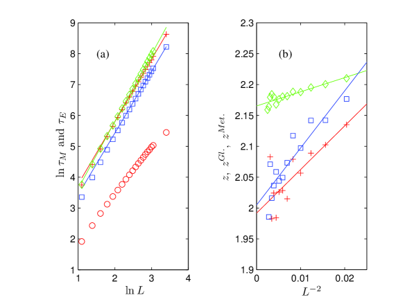
Figure 1: (a) Values of $\ln\tau_{M}$ for Glauber dynamics obtained from the results reported in Ref. Nightingale00 ($\diamond$) and values obtained from $T(M;M^{\prime})$ (+) as a function of $\ln L$. We also plot $\ln\tau_{M}$ for the Metropolis et al. dynamics ($\Box$) and $\tau_{E}$ for the Glauber dynamics obtained from the matrix $T(E;E^{\prime})$ ($\circ$). The fitted straight lines were obtained neglecting data for $L<15$ and have slopes $z^{Gl.}=2.02$, $z^{Met.}=2.00$ and $z=2.18$. (b) Estimations of the dynamic critical exponent from the local slopes of the graph in (a) as a function of $L^{-2}$. The symbols are as in (a). The extrapolated exponents are $z^{Gl.}=1.991$, $z^{Met.}=2.00$ and $z=2.165$.

In Fig. 2(a) we plot the relaxation times obtained from $T(M;M^{\prime})$ for the Metropolis et al. dynamics in the flat energy-magnetization ensembles, flat energy ensemble and flat magnetization ensemble. The fitted straight lines have slopes given by $z^{M}_{E,M}=2.11$, $z^{M}_{E}=2.69$ and $z^{M}_{M}=1.99$, respectively. In Fig. 2(b) we plot the relaxation times obtained from $T(E;E^{\prime})$ for the Metropolis et al. dynamics in the same ensembles. The slopes of the fitted straight lines are $z^{E}_{E,M}=2.14$, $z^{E}_{E}=2.13$ and $z^{E}_{M}=1.99$, respectively. We neglected the data for $L<15$ in all the fits shown in Figs. 2 (a) and (b).

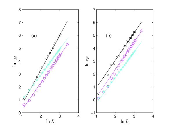
Figure 2: Relaxation times obtained for the Metropolis et al. dynamics in the flat energy-magnetization ensemble ($\circ$), flat magnetization ensemble ($*$) and flat energy ensemble ($\times$). In (a) we plot $\tau_{M}$ obtained from $T(M;M^{\prime})$ and the fitted straight lines have slopes $z^{M}_{E,M}=2.11$, $z^{M}_{E}=2.69$ and $z^{M}_{M}=1.99$. In (b) we plot $\tau_{E}$ obtained from $T(E;E^{\prime})$ and the fitted straight lines have slopes $z^{E}_{E,M}=2.14$, $z^{E}_{E}=2.13$ and $z^{E}_{M}=1.99$. Both in (a) and (b) data for $L<15$ were neglected in the fits.

In Fig. 3(a) we show the estimation of the dynamic exponent from the local slopes of the relaxation time plots in the magnetization projected space (Fig. 2(a)) as a function of $L^{-2}$. The estimates for $z_{E}^{M}$ (flat energy histogram) in Fig. 3(a) seem to have converged for the system sizes studied. The average value for system sides $L\geq 15$ is $z^{M}_{E}=2.68(2)$. This result is compatible with the availableguerra2004 result $z=2.80(13)$ obtained by a Monte Carlo estimate of the convergence time of the time-dependent energy histogram to the stationary flat distribution of the energy. The estimates for $z_{M}^{M}$ (flat magnetization histogram) plotted in the same figure show a dependence with system size approaching a value close to 2 for infinite system sides. The infinite size extrapolation for $z_{E,M}^{M}$ (flat energy and magnetization histogram) gives a value slightly larger than 2, $z^{M}_{E,M}=2.08$. For this multicanonical dynamics the results show an even-odd effect and it is important to do separate estimates for even and odd system sides. In Fig. 3(b) we also show the estimation of the dynamic exponent from the local slopes of the plots (Fig. 2(b)) for the energy projected dynamics. The infinite size extrapolation for $z_{E,M}^{E}$ for even and odd system side are very close to each other and given by, $z_{E,M}^{E}=2.07$. The extrapolations for $z_{E}^{E}$ for odd system side and even system side give $z_{E}^{E}=2.07$ and $1.99$,respectively. The difference between these two estimates may be a sign of the presence of corrections to scaling not properly accounted by our analysis. The estimates for $z_{M}^{E}$ show a size dependence that is compatible with a value close to 2.

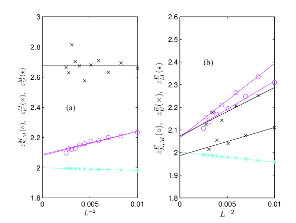
Figure 3: (a) Dynamic exponent estimates $z_{E,M}^{M}(\circ),\ \ z_{E}^{M}(\times),\ \ z_{M}^{M}(*)$ from local slopes of the plots shown in Fig. 2 (a) as a function of $L^{-2}$. For the estimates for the energy-magnetization flat multicanonical ensemble we made separate estimations for even and odd $L$ system sides. The infinite system size extrapolations give, $z_{E,M}^{M}=2.08$, $z_{E}^{M}=2.68$ and $z_{M}^{M}=2.00$. (b) $z_{E,M}^{E}(\circ),\ \ z_{E}^{E}(\times),\ \ z_{M}^{E}(*)$ from local slopes of the plots shown in Fig. 2 (b) as a function of $L^{-2}$. For the estimates for the flat $(E,M)$ ensemble and for the flat energy ensemble we made separate estimations for even and odd $L$ system sides. The infinite system size extrapolations give, $z_{E,M}^{E}=2.07$, $z_{E}^{E}=2.07$ and $1.99$ for odd and even L, respectively, and $z_{M}^{E}=2.00$.

The full state transition rate matrix $W$, in the flat magnetization ensemble is lumpable with respect to the classification of the states according to their magnetization. Consequently, the result $z^{M}_{M}=2.00$ does not suffer from the approximation inherent to the projection procedure. A sufficient and necessary condition for lumpabilityKemeny76 , is that the total probability to go from a state belonging to a given magnetization class to another class with different magnetization is the same for every state in the starting class. For each state in the starting class with magnetization M there are $n_{\pm}$ states in the final class $M\pm 2$ where $n_{\pm}$ is the number of up/down spins in the initial configuration. The probability to move to each of these final states in the final class has a constant value that depends only on the initial $M$ and on the final $M\pm 2$. All the states in the starting class have the same number of up spins and down spins so the probability to move to $M\pm 2$ is the same for every state in the starting class. The matrix $T(M;M^{\prime})$ is a tridiagonal symmetric matrix with matrix elements given by, $T(M+2;M)=T(M;M+2)=\frac{n_{+}+1}{N}$ for $M<0$, and $T(M+2;M)=T(M;M+2)=\frac{n_{-}}{N}$ for $M\geq 0$.

V Magnetization tunnelling times

As a measure of performance for multicanonical methods the average tunnelling times were introduceddayal2004 . These tunnelling times measure the time required to sample the whole phase space and scale with system size differently than the relaxation time. It was shown that it is important to distinguish between tunnelling from ground-sate to maximum energy, the up direction, and from the high energy to the ground-state, the down directioncosta2005 .

All the tunnelling times reported by us are calculated for the projected dynamics associated with $T(M;M^{\prime})$. We calculate the average time, $\tau_{t}$ for the system to go from magnetization $M=-N$ to $M=N$. We also consider two other average times: The time $\tau_{u}$ for the system to go from $M=-N$ to zero magnetization, and the time $\tau_{d}$ for the system to go either to $M=+N$ or $M=-N$ when it starts from $M=0$. This definition of $\tau_{u}$ and $\tau_{d}$ apply only to systems with even $L$ (and $N$) such that $M=0$ is an accessible value of the magnetization.

The tunnelling times above defined obey the relation $\tau_{u}+\tau_{d}=\tau_{t}/2$ that follows from the following simple argument: For the system to go from $M=-N$ to $M=N$ it has to reach $M=0$ at some point. It will do so for the first time using an average time $\tau_{u}$. Then with probability $1/2$ it will reach for the first time $M=N$ and the tunnelling time would be $\tau_{u}+\tau_{d}$ or it will return to $M=-N$ and it will reach later $M=N$ taking a time $\tau_{t}$. Consequently the tunnelling times obey the relation $\frac{1}{2}(\tau_{u}+\tau_{d})+\frac{1}{2}\tau_{t}=\tau_{t}$. This argument uses the fact that the matrix $T(M;M^{\prime})$ has the symmetry property $T(M\pm 2;M)=T(-M\mp 2;-M)$ and so the walk along positive values of the magnetization has the same statistical properties of the walk along negative values of the magnetization.

The time to go from $M=-N$ to $M=N$ can be easily computed taking advantage of the fact that $T(M;M^{\prime})$ is non zero only when $M=M^{\prime}\pm 2$ and $M^{\prime}=M$. If we do not allow transitions from $M=N$ to $M=N-2$ the $M=N$ becomes an absorbing site for every walk along the magnetization axis meaning that it will end there upon a first visit. Defining $h(M)$ as the average time spent at magnetization value $M$ Novotny01 , we can write:

$$h(M-2)T(M;M-2)-h(M)T(M-2;M)=1$$ (23)

which means that the difference between the average number of jumps in the positive direction ($M-2\rightarrow M$) and the average number of jumps in the negative direction ($M\rightarrow M-2$) should be equal to one since the system will eventually reach $M=N$ by moving one time in excess in the positive direction through the bond connecting the sites $M-2$ and $M$. At $M=N$ there are no jumps in the negative direction and so $h(N-2)T(N;N-2)=1$. It is then simple to calculate $h(M)$ and the average tunnelling time for the system to go from $M=-N$ to $M=N$ is given by,$\tau_{t}=\sum_{M=-N}^{M=N-2}h(M)$.

The time $\tau_{u}$ to reach for the first time $M=0$ starting from $M=-N$ is obtained using the recursion (23) together with the equation $h(-2)T(0;-2)=1$ to get $\tau_{u}=\sum_{M=-N}^{M=-2}h(M)$. Finally, the average time required to start from $M=0$ and reach for the first time either $M=-N$ or $M=N$, $\tau_{d}$ is obtained from the recursion

$$h(M)T(M-2;M)-h(M-2)T(M;M-2)=1$$ (24)

with a modified rate $T(-2;0)$ equal to $T(-2;0)+T(2;0)$ and $h(-N+2)T(-N;-N+2)=1$. The average time $\tau_{d}$ is then given by $\tau_{d}=\sum_{M=-N+2}^{M=0}h(M)$. The average tunnelling times obtained by this method could also have been obtained from the calculation of the probability of first visit to the absorbing site that can be computed from the eigenstates and eigenvectors of the associated absorbing Markov chain matrix ( see costa2005 ).

The tunnelling times are characterized by dynamic exponentsdayal2004 , $\tau_{t}\sim L^{d+z_{t}}$, $\tau_{u}\sim L^{d+z_{u}}$, $\tau_{d}\sim L^{d+z_{d}}$. The relation between these tunnelling times imply that $z_{t}$ is equal to the biggest of the two exponents, $z_{u}$ and $z_{d}$, $z_{t}=\max(z_{d},z_{u})$. Note that the tunnelling times reported by us are measured in units of lattice sweeps and not in units of single site updates.

In Fig. 4(a) we show the size dependence of the tunnelling times, $\tau_{t}$, $\tau_{u}$ and $\tau_{d}$ for the Metropolis et al. dynamics in a flat magnetization-energy histogram ensemble obtained from the matrix $T(M;M^{\prime})$. We see that $\tau_{t}\sim\tau_{d}\gg\tau_{u}$. The scaling exponent of $\tau_{u}$ obtained from the plot is $z_{u}=0.15$ which predicts a scaling $\tau_{u}\sim L^{2.15}$ close to the exponent of the relaxation time $z^{M}_{E,M}=2.11$ reported in the previous section. This behavior is similar to the one found in costa2005 where $\tau_{u}$ (in the energy space) was found to scale like the relaxation time of the system. For the other two exponents we have obtained $z_{t}\sim z_{d}\sim 2.12$. Note that for a random walk in the magnetization axis a value for these exponents equal to 0 is expected. In Fig. 4(b) we show the local slopes for the plots in Fig. 4(a) as a function of $L^{-2}$. The estimates for $z_{t}$ and $z_{d}$ seem to follow a straight line predicting an infinite system value $2.11$ and $2.08$, respectively. The infinite size extrapolation for $z_{u}$ is $0.14$.

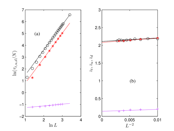
Figure 4: (a) Tunnelling times, $\tau_{t}$ ($\circ$), $\tau_{u}$(+) and $\tau_{d}$ (*) as a function of system size $L$ for the Metropolis et al. dynamics in a flat magnetization-energy histogram ensemble obtained from the matrix $T(M;M^{\prime})$. The fitted straight lines were obtained neglecting data for $L<15$ and have slopes, $z_{t}=2.12$, $z_{u}=0.15$ and $z_{d}=2.12$, respectively. In (b) we plot the corresponding local slopes as a function of $L^{-2}$. Even and odd system sides were treated separately. The infinite system extrapolation gives, $z_{t}=2.11$, $z_{u}=0.14$ and $z_{d}=2.08$.

In Fig. 5(a) we show the size dependence of the tunnelling times, $\tau_{t}$, $\tau_{u}$ and $\tau_{d}$ for the Metropolis et al. dynamics in a flat energy histogram ensemble obtained from the matrix $T(M;M^{\prime})$. The slopes of the fitted straight lines give $z_{t}=0.69$, $z_{u}=0.64$ and $z_{d}=0.63$. The result for $z_{t}$ can be compared with the value $0.78$ reported in Ref. vianalopes2006 and the value $0.743(7)$ reported in Ref. dayal2004 by measuring average times for energy excursions. An exponent $z_{u}=0.6$, also obtained from Monte-Carlo estimates of energy tunnelling times was previously reportedtesejoao in very good agreement with our result. In Fig. 5(b) we make infinite size extrapolations giving, $z_{t}=0.70$ and 0.65 for odd and even system sides, respectively, $z_{u}=0.63$ and $z_{d}=0.66$.

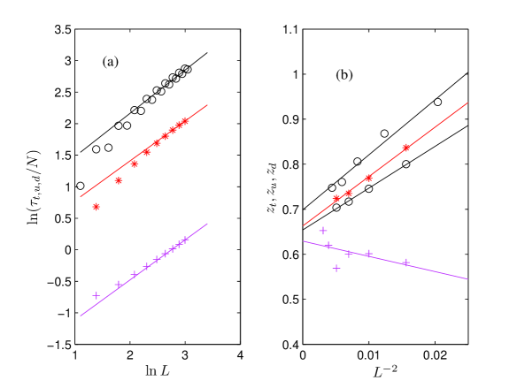
Figure 5: (a) Tunnelling times, $\tau_{t}$ ($\circ$), $\tau_{u}$(+) and $\tau_{d}$ (*) as a function of system size $L$ for the Metropolis et al. dynamics in a flat energy histogram ensemble obtained from the matrix $T(M;M^{\prime})$. The fitted straight lines were obtained neglecting data for $L<15$ and have slopes, $z_{t}=0.69$, $z_{u}=0.64$ and $z_{d}=0.63$, respectively. In (b) we plot the corresponding local slopes as a function of $L^{-2}$. For the $z_{t}$ estimates even and odd system sides were treated separately. The infinite size extrapolations are, $z_{t}=0.70$ and 0.65 for odd and even system sides, respectively, $z_{u}=0.63$ and $z_{d}=0.66$.

Finally, we consider the Metropolis et al. dynamics for the flat magnetization histogram ensemble. For this case it is possible to compute analytically the tunnelling times from the recursion relations given above, Eqs. (23,24) and the knowledge of the matrix $T(M;M^{\prime})$. The analytical results are, $\tau_{u}=N/2$, $\tau_{t}=(N+1)H(N/2)$ and $\tau_{d}=\frac{1}{2}\bigl{(}(N+1)H(N/2)-N\bigr{)}$ where, $H(n)=\sum_{k=1}^{n}1/k$ is the Harmonic number. Using the known asymptotic result, for large $n$, $H(n)\sim(\ln n+\gamma)$ where $\gamma=0.5772156649...$ is the Euler constant we have asymptotic expressions for the tunnelling times that predict, $\tau_{t}/N\sim\tau_{d}/N\sim\ln N$ and the tunnelling exponents are, $z_{t}=z_{d}=z_{u}=0$. In Fig. 6(a) we compare the numerical results for the tunnelling times, $\tau_{t}$, $\tau_{u}$ and $\tau_{d}$ with the analytical results. Note that, because of the logarithmic dependence of $\tau_{t}$ and $\tau_{u}$ the estimates for the exponents $z_{t}$ and $z_{d}$ that we could obtain for the slopes of the data shown in Fig. 6(a) give effective values around $0.35$ that would slowly approach zero only if larger systems were considered.

From the three multicanonical ensembles studied we see that the flat magnetization ensemble is the one with smaller tunnelling exponents and relaxation time exponent. Recently, it was shown that it is possible to optimize the ensemble in multicanonical simulations such that the tunnelling exponent, $z_{t}$ is also reduced to zerotrebst2004 ; vianalopes2006 .

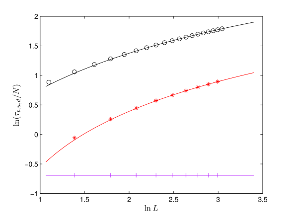
Figure 6: (a) Tunnelling times, $\tau_{t}$ ($\circ$), $\tau_{u}$(+) and $\tau_{d}$ (*) as a function of system size $L$ for the Metropolis et al. dynamics in a flat magnetization histogram ensemble obtained from the matrix $T(M;M^{\prime})$. The lines are the analytical asymptotic results given in the text.

VI Concluding Remarks

We have shown that projected dynamics in the magnetization space is a reasonably good approximation to the full state space single spin flip dynamics studied in this work: canonical ensemble Glauber and Metropolis et al. dynamics and three multicanonical ensemble dynamics with flat energy-magnetization, flat energy and flat magnetization histograms. The energy projected dynamics is generally a worse approximation being not able to preserve the power-law size increase of the relaxation time for canonical ensemble dynamics. From all the studied dynamics only the flat energy histogram dynamics show a z exponent clearly larger than 2 and near $2.7$. For the case of the flat magnetization histogram the projection in the magnetization space is exact and it is possible to obtain analytical results for the tunnelling times predicting a zero value for the exponents, $z_{t},z_{d}$ and $z_{u}$. The tunnelling exponents, $z_{t}$ (and $z_{d}$) for the energy and magnetization flat histogram ensemble are much bigger, $z_{t}=z_{d}\sim 2$ and larger than the exponent $z_{u}\sim 0$. For the flat energy histogram dynamics these three exponents are not very different and the estimates fall between the values, $z_{u}\sim 0.63$ and $z_{t}\sim 0.70$ for odd system sides. These results were obtained from the tunnelling properties of the projected dynamics in the magnetization space that were found to be in rough agreement with ones obtained by independent methods for excursions in the energy space for the flat energy multicanonical ensemble.

Finally, the results show that the evaluation of the relative performance of single-spin flip dynamics in Ising like models can be done very efficiently by studying the projected dynamics in the magnetization space: the approximation gives reasonably accurate dynamic exponents; any, arbitrary, single-spin flip dynamics can be studied from Monte-Carlo estimations of $T_{\infty}(E,M;E^{\prime},M^{\prime})$ for several system sizes in the energy-magnetization space and the large dimensional reduction achieved by the projection in the magnetization space allows the application of matrix diagonalization techniques for bigger system sizes.

Furthermore, the application of projection methods to cluster dynamics in Ising models and also to other models projected along their slowest mode may be of considerable interest.

- (1) P. C. Hohenberg and B. I. Halperin Rev. Mod. Phys. 49, 435 (1977).
- (2) A.D. Sokal, in C. DeWitt-Morette, P. Cartier and A. Folacci, eds., Functional Integration: Basics and Applications (Plenum, New York, 1997), pp. 131 192.
- (3) M. P. Nightingale and H. W. J. Blöte, Phys. Rev. Lett. 76, 4548 (1996).
- (4) M. P. Nightingale and H. W. J. Bl te, Phys. Rev. B 62, 1089 (2000).
- (5) R H Swendsen and J S Wang, Phys. Rev. Lett. 58,86 (1987).
- (6) U. Wolff, Phys Rev. Lett. 62,361 (1989).
- (7) B A Berg and T. Neuhaus, Phys. Rev. Lett 68, 9 (1992).
- (8) J. Lee Phys.Rev. Lett 71, 211 (1993).
- (9) G.Bhanot, R.Salvador, S.Black, P.Carter and R.Toral, Phy. Rev. Lett. 59, 803 (1987).
- (10) J. Lee, M. A. Novotny, and P. A. Rikvold, Phys. Rev. E 52, 356 (1995).
- (11) I. Shteto, J. Linares, and F. Varret, Phys. Rev. E 56 5128 (1997).
- (12) I. Shteto, K. Boukheddaden, and F. Varret, Phys. Rev. E 60 5139 (1999).
- (13) M. Kolesik, M. A. Novotny, and P. A. Rikvold, Phys. Rev. Lett. 80, 3384 (1998).
- (14) M. A. Novotny M.A. Novotny, Annual Reviews of Computational Physics IX, edited by D. Stauffer, (World Scientific, Singapore, 2001), pages 153-210.
- (15) M Kolesik, M. A. Novotny, P. A. Rikvold and D. M. Townsley, in Computer simulation studies in Condensed Matter Physics X, edited by D. P. Landau, K.K. Mon and H.-B. Schüuttler (Springer, Berlin, 1998), 246.
- (16) J. G. Kemeny and J. L. Snell, Finite Markopv Chains, (Springer, New York, 1976).
- (17) J. S. Wang, T. K. Tay and R. H. Swendsen, Phys.Rev.Lett, 82, 476 (1999).
- (18) J. S. Wang and R. H. Swendsen, J. Stat. Phys. 106, 245 (2002).
- (19) N. Metropolis et. al, J. Chem Physics, 21, 1087-92 (1958); R. J. Glauber, J. of Math. Physycs 4, 294-307 (1963)
- (20) P Dayal et. al, Phys. Rev. Lett. 92, 097201 (2004).
- (21) M D Costa, J V Lopes and J M B Lopes dos Santos, Eur. Phys. Lett. 72(5), 802-808 (2005).
- (22) P. D. Beale Phys. Rev. Lett. 76, 78 (1996).
- (23) P M C de Oliveira, Braz. J. Phys. 30, 195 (2000).
- (24) A Bortz, M H Kalos and J L Lebowitz, J. Comp. Phys. 17(1), 10-18 (1975).
- (25) E. Domany, Phys. Rev. Lett. 52, 871,(1984).
- (26) M Arjunwadkara, et. al. Physica A 323, 487-503 (1995).
- (27) M L Guerra and J D Muñoz, Int. J. Mod. Physics C, 15(3):471-478 (2004).
- (28) J V Lopes M.D. Costa, J.M.B. Lopes dos Santos and R. Toral, Phys. Rev. E 74, 046702 (2006).
- (29) J V Lopes, Phd Thesis, Universidade do Porto (2006).
- (30) S Trebst, D Huse, and M. Troyer, Phys. Rev. E 70, 046701 (2004).