Ab initio calculations of third-order elastic constants and related properties for selected semiconductors

Abstract

We present theoretical studies for the third-order elastic constants $C_{ijk}$ in zinc-blende nitrides AlN, GaN, and InN. Our predictions for these compounds are based on detailed ab initio calculations of strain-energy and strain-stress relations in the framework of the density functional theory. To judge the computational accuracy, we compare the ab initio calculated results for $C_{ijk}$ with experimental data available for Si and GaAs. We also underline the relation of the third-order elastic constants to other quantities characterizing anharmonic behaviour of materials, such as pressure derivatives of the second-order elastic constants $c^{\prime}_{ij}$ and the mode Grüneisen constants for long-wavelength acoustic modes $\gamma({\bf q},{\bf j})$.
Paper accepted to Phys. Rev. B.

I Introduction

Third-order elastic constants $C_{ijk}$ are important quantities characterizing nonlinear elastic properties of materials and the interest in them dates back to the beginning of modern solid state physics. Birch (1947); Murnaghan (1951); Bhagavantam (1966); Thurston and Brugger (1964); Brugger (1964) Third- and higher-order elastic constants are useful not only in describing mechanical phenomena when large stresses and strains are involved (e.g., in heterostructures of optoelectronic devices), but they can also serve as a basis for discussion of other anharmonic properties. The applications include phenomena such as thermal expansion, temperature dependence of elastic properties, phonon-phonon interactions etc. Hiki (1981)

As far as theoretical studies are concerned, at the beginning the third-order elastic constants were calculated in the framework of the valence force Keating model. Keating (1966) Later on, many other more sophisticated microscopic theories were employed to describe and predict nonlinear elastic properties of crystals on the basis of their atomic composition.Hiki (1981) Nowadays, precise ab initio calculations seem to be the most promising approach to handle this task. Such applications of density functional theory (DFT) on the local density approximation level (LDA) were already reported. Nielsen and Martin (1985); Sörgel and Scherz (1998)

Recently, one observes increased interest in nonlinear effects in elastic Kato and Hama (1994); Łepkowski and Majewski (2004); Łepkowski et al. (2005) and piezoelectric properties. Shimada et al. (1998); Bester et al. (2006) This is strongly connected to the fact that research focuses nowadays on the semiconductor nanostructures. In such systems these nonlinear effects are not only more pronounced than in bulk materials, but very often their reliable quantitative description is a prerequisite for correct theoretical explanation of the experimental data. Frogley et al. (2000); Ellaway and Faux (2002); Ma et al. (2004); Luo et al. (2005); Łepkowski et al. (2005); Bester et al. (2006) In this paper, we perform ab initio calculations of the unknown third-order elastic constants in cubic nitrides. The nitrides are technologically important group of materials for which the nonlinear effects are particularly significant. Kato and Hama (1994); Vaschenko et al. (2003); Łepkowski et al. (2005); Łepkowski and Majewski (2006) Therefore, the knowledge of the third-order elastic moduli will definitely improve the modeling of nitride based nanostructures. In this work we also briefly discuss the applications of $C_{ijk}$ to determination of other anharmonic properties, namely, pressure derivatives of second-order elastic moduli $c^{\prime}_{ij}$ and mode Grüneisen constants $\gamma({\bf q},{\bf j})$. Since the third-order effects are rather subtle, their computational determination can also serve as a precise test of accuracy for modern ab initio codes based on DFT approach.

The paper is organized as follows. In Sec. II we give a general overview of the nonlinear elasticity theory. Sec. III contains a description of employed methodology. Also results for third-order elastic constants obtained from ab initio calculations are presented there. Our findings for Si and GaAs are compared with previous numerical calculations and measurements, later on theoretical predictions for zinc-blende nitrides AlN, GaN, and InN are given. Secs. IV and V deal with the determination of quantities related to third-order elastic constants, namely, the pressure dependent elastic constants and mode Grüneisen constants, respectively. Finally, we conclude the paper in Sec. VI.

II Overview of nonlinear elasticity theory

Here we will recall some basic facts from nonlinear theory of elasticity. Birch (1947); Murnaghan (1951); Bhagavantam (1966); Thurston and Brugger (1964); Brugger (1964); Hiki (1981) Let us consider point ${\bf a}$ which, after applying strain to a crystal, moves to the position ${\bf x}$. After introducing the Jacobian matrix ${\bf J}$

$$J_{ij}=\frac{\partial x_{i}}{\partial a_{j}}$$ (1)

we may define the Lagrangian strain

$$\bm{\eta}=\frac{1}{2}(\bm{J}^{T}\bm{J}-{\bf 1}),$$ (2)

which is a convenient measure of deformation for an elastic body.

The energy per unit mass $E(\bm{\eta})$ corresponding to the applied strain may be developed in power series with respect to $\bm{\eta}$. This leads to the expression

$$\rho_{0}E(\bm{\eta})=\frac{1}{2!}\sum_{i,j=1,6}c_{ij}\eta_{i}\eta_{j}+\frac{1}{3!}\sum_{i,j,k=1,6}C_{ijk}\eta_{i}\eta_{j}\eta_{k}+\dots,$$ (3)

where we applied Voigt convention ($\eta_{11}\to\eta_{1}$, $\eta_{22}\to\eta_{2}$, $\eta_{33}\to\eta_{3}$, $\eta_{23}\to\eta_{4}/2$, $\eta_{13}\to\eta_{5}/2$, $\eta_{12}\to\eta_{6}/2$) and introduced the density of unstrained crystal $\rho_{0}$. The $c_{ij}$ and $C_{ijk}$ denote here second- and third-order elastic constants respectively. If we introduce $\bm{J}=(\bm{1}+\bm{\epsilon})$ and assume that $\bm{\epsilon}$ is symmetric (rotation free) linear strain tensor, the definition of $\eta$ [Eq. (2)] yields

$$\bm{\eta}=\bm{\epsilon}+\frac{1}{2}\bm{\epsilon}^{2}.$$ (4)

Substituting the above result to the expansion in Eq. (3) and leaving only terms up to second order with respect to components of $\bm{\epsilon}$ recover the infinitesimal theory of elasticity.

Naturally, the general expression for energy of strained crystal, as given by Eq. (3), can be simplified by employing symmetry considerations. For cubic crystals, this procedure yields the following formula:

$$\rho_{0}E(\bm{\eta}) = \frac{1}{2}c_{11}\left(\eta_{1}^{2}+\eta_{2}^{2}+\eta_{3}^{2}\right)+\frac{1}{2}c_{44}\left(\eta_{4}^{2}+\eta_{5}^{2}+\eta_{6}^{2}\right)+$$

$$+c_{12}(\eta_{1}\eta_{2}+\eta_{3}\eta_{2}+\eta_{1}\eta_{3})+$$

$$\frac{1}{6}C_{111}\left(\eta_{1}^{3}+\eta_{2}^{3}+\eta_{3}^{3}\right)+$$

$$\frac{1}{2}C_{112}\left(\eta_{2}\eta_{1}^{2}+\eta_{3}\eta_{1}^{2}+\eta_{2}^{2}\eta_{1}+\eta_{3}^{2}\eta_{1}+\eta_{2}\eta_{3}^{2}+\eta_{2}^{2}\eta_{3}\right)+$$

$$C_{123}\eta_{1}\eta_{2}\eta_{3}+\frac{1}{2}C_{144}\left(\eta_{1}\eta_{4}^{2}+\eta_{2}\eta_{5}^{2}+\eta_{3}\eta_{6}^{2}\right)+$$

$$\frac{1}{2}C_{155}\left(\eta_{2}\eta_{4}^{2}+\eta_{3}\eta_{4}^{2}+\eta_{1}\eta_{5}^{2}+\eta_{3}\eta_{5}^{2}+\eta_{1}\eta_{6}^{2}+\eta_{2}\eta_{6}^{2}\right)+$$

$$C_{456}\eta_{4}\eta_{5}\eta_{6}+\dots$$

Another fundamental quantity in the theory of finite deformations is Lagrangian stress

$$t_{ij}=\rho_{0}\frac{\partial E}{\partial\eta_{ij}},$$ (6)

which can be expressed in terms of linear stress tensor $\bm{\sigma}$ using the following formula

$$\bm{t}=\det(\bm{J})\bm{J}^{-1}\bm{\sigma}\left(\bm{J}^{T}\right)^{-1}.$$ (7)

Again, Voigt convention ($t_{11}\to t_{1}$, $t_{22}\to t_{2}$, $t_{33}\to t_{3}$, $t_{23}\to t_{4}$, $t_{13}\to t_{5}$, $t_{12}\to t_{6}$) is used here.

III Determination of third-order elastic constants

III.1 Methodology and computational details

In this work, we have determined third-order elastic constants for Si, GaAs, and zinc-blende nitrides (AlN, GaN, and InN) on the basis of quantum DFT calculations for deformed crystals. The results were obtained in two ways - employing strain-energy formula [Eq. (II)] and from strain-stress relation [Eqs. (6) and (7)].

The detailed procedure was as follows. We considered six sets of deformations parametrized by $\eta$

$$\bm{\eta}_{A} = (\eta,0,0,0,0,0),$$

$$\bm{\eta}_{B} = (\eta,\eta,0,0,0,0),$$

$$\bm{\eta}_{C} = (\eta,0,0,\eta,0,0),$$

$$\bm{\eta}_{D} = (\eta,0,0,0,\eta,0),$$ (8)

$$\bm{\eta}_{E} = (\eta,\eta,\eta,0,0,0),$$

$$\bm{\eta}_{F} = (0,0,0,\eta,\eta,\eta).$$

In every case, $\eta$ was varied between $-0.08$ and $0.08$ with step $0.008$. For every deformed configuration, the positions of atoms were optimized and both energy and stress tensors were calculated on the basis of quantum DFT formalism. In this way, for each type of distortion, dependencies of energy $E(\eta)$ and stress tensor $\bm{t}(\eta)$ on strain parameter $\eta$ were obtained. The numerical results have been in turn compared with the expressions from the nonlinear theory of elasticity, which are summarized in Table 1. This allows to extract the values of the second- and third-order elastic constants, by performing suitable polynomial fits.

Table 1: Dependencies of energy and stress on deformation parameter $\eta$ for considered types of deformation $\bm{\eta}_{A},\dots,\bm{\eta}_{F}$, which have been used to determine second- and third-order elastic constants.

Energy:
	$\rho_{0}E(\bm{\eta}_{A})=\frac{1}{6}C_{111}\eta^{3}+\frac{1}{2}c_{11}\eta^{2}\doteq f_{A}(\eta)$
	$\rho_{0}E(\bm{\eta}_{B})=\left(\frac{1}{3}C_{111}+C_{112}\right)\eta^{3}+(c_{11}+c_{12})\eta^{2}\doteq f_{B}(\eta)$
	$\rho_{0}E(\bm{\eta}_{C})=\left(\frac{1}{6}C_{111}+\frac{1}{2}C_{144}\right)\eta^{3}+\left(\frac{1}{2}c_{11}+\frac{1}{2}c_{44}\right)\eta^{2}\doteq f_{C}(\eta)$
	$\rho_{0}E(\bm{\eta}_{D})=\left(\frac{1}{6}C_{111}+\frac{1}{2}C_{155}\right)\eta^{3}+\left(\frac{1}{2}c_{11}+\frac{1}{2}c_{44}\right)\eta^{2}\doteq f_{D}(\eta)$
	$\rho_{0}E(\bm{\eta}_{E})=\left(\frac{1}{2}C_{111}+3C_{112}+C_{123}\right)\eta^{3}+\left(\frac{3}{2}c_{11}+3c_{12}\right)\eta^{2}\doteq f_{E}(\eta)$
	$\rho_{0}E(\bm{\eta}_{F})=C_{456}\eta^{3}+\frac{3}{2}c_{44}\eta^{2}\doteq f_{F}(\eta)$
Stress:
	$t_{1}(\bm{\eta}_{A})=\frac{1}{2}C_{111}\eta^{2}+c_{11}\eta\doteq g_{A1}(\eta)$
	$t_{2}(\bm{\eta}_{A})=\frac{1}{2}C_{112}\eta^{2}+c_{12}\eta\doteq g_{A2}(\eta)$
	$t_{3}(\bm{\eta}_{B})=\left(C_{123}+C_{112}\right)\eta^{2}+2c_{12}\eta\doteq g_{B}(\eta)$
	$t_{4}(\bm{\eta}_{C})=C_{144}\eta^{2}+c_{44}\eta\doteq g_{C}(\eta)$
	$t_{5}(\bm{\eta}_{D})=C_{155}\eta^{2}+c_{44}\eta\doteq g_{D}(\eta)$
	$t_{4}(\bm{\eta}_{F})=C_{456}\eta^{2}+c_{44}\eta\doteq g_{F}(\eta)$

The DFT calculations have been performed using the ab initio total energy code VASP developed at the Institut für Materialphysik of Universität Wien. Kresse and Hafner (1993); Kresse and Furthmüller (1996, 1996) The projector augmented wave (PAW) approach Blöchl (1994) has been used in its variant available in the VASP package. Kresse and Joubert (1999) For the exchange-correlation functional generalized gradient approximation (GGA) according to Perdew, Burke and Ernzerhof (PBE) Perdew et al. (1996a, b) has been applied. For Ga and In, semicore 3d and 4d electrons have been explicitly included in the calculations.

Since the determination of subtle third-order effects requires high precision, we have performed careful convergence tests for parameters governing the accuracy of computations. On the basis of our tests we have chosen the following energy cutoffs $E_{\rm{cutoff}}^{\rm{Si}}=600\;\rm{eV}$, $E_{\rm{cutoff}}^{\rm{GaAs}}=700\;\rm{eV}$, and $E_{\rm{cutoff}}^{\rm{AlN}}=E_{\rm{cutoff}}^{\rm{GaN}}=E_{\rm{cutoff}}^{\rm{InN}}=800\;\rm{eV}$. For the Brillouin zone integrals we have followed the Monkhorst-Pack schemeMonkhorst and Pack (1976), in Si and GaAs we have used $13\times 13\times 13$ mesh, whereas for AlN, GaN, and InN we have applied $11\times 11\times 11$ sampling. One example of performed tests for GaN is presented in Fig. 1. It illustrates the dependence of two sample elastic moduli $C_{111}$ and $C_{144}$ on the energy cutoff and density of Monkhorst-Pack k-point mesh. For the chosen parameters ($E_{\rm{cutoff}}^{\rm{GaN}}=800\;\rm{eV}$ and $11\times 11\times 11$ k-point mesh) the difference between successive values of examined constants in our test is lower than $1\;\rm{GPa}$. This difference is smaller than e.g. discrepancies observed between results obtained from strain-energy and strain-stress approach which, in the opinion of the authors, indicates that the convergence with respect to parameters responsible for numerical accuracy is very reasonable.

Figure 1: Sample convergence tests for the third-order elastic constants in zinc-blende GaN. Panel (a) illustrates the dependence of $C_{111}$ and $C_{144}$ on energy cutoff (Monkhorst-Pack sampling $11\times 11\times 11$ was applied for all points). Panel (b) shows the analogous dependence on the density of k-points mesh (energy cutoff 800 eV was used for all points). Note different scales for $C_{111}$ and $C_{144}$. Later on, all calculations for GaN have been performed with the energy cutoff 800 eV and the Monkhorst-Pack sampling $11\times 11\times 11$.

III.2 Results and discussion

Results are presented in Tables 2 and 3. Table 2 contains our findings for benchmark materials Si and GaAs, accompanied by available experimental data and previous theoretical findings within LDA-DFT theory. Table 3 gives our prediction for the unknown values of $C_{ijk}$ for cubic nitrides. For completeness, we also provide there our prediction for second-order elastic moduli and compare them with previous calculations. Łepkowski et al. (2005) For $c_{ij}$ values, sometimes it was possible to determine one constant from a few fits [e.g., $c_{44}$ from coefficients in $f_{C}(\eta)$, $f_{D}(\eta)$, and $f_{F}(\eta)$], obtaining slightly different results [e.g., for GaN, $c_{44}=145,151,147$ GPa from $f_{C}(\eta)$, $f_{D}(\eta)$, and $f_{F}(\eta)$ respectively]. In such cases the average of all obtained values was given in the tables. The sample plots of both energy and stress dependencies for GaN together with fitted polynomials are depicted in Figs. 2 and 3.

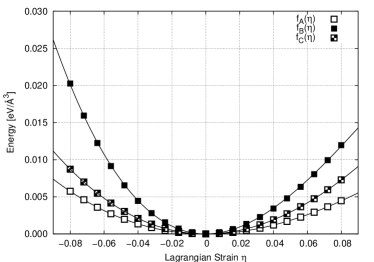
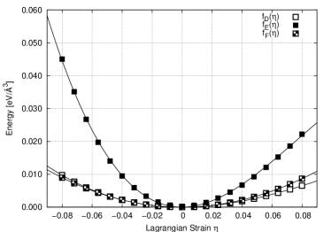
Figure 2: Plots of strain-energy relations for GaN. Squares denote results of DFT computations, solid line represents a polynomial fit. See main text for details and Table 1 for definitions of $f_{A}(\eta)$,$f_{B}(\eta)$,…,$f_{F}(\eta)$.

Figure 3: Plots of strain-stress relations for GaN. Circles denote results of DFT computations, solid line represents a polynomial fit. See main text for details and Table 1 for definitions of $g_{A1}(\eta)$,$g_{A2}(\eta)$,…, $g_{F}(\eta)$). Curves for $g_{C}(\eta)$ and $g_{F}(\eta)$ coincide because of very similar values of $C_{144}$ and $C_{456}$ in GaN.

When analyzing the above results, one has to bear in mind that both measurements and calculations of the third-order elastic constants are difficult. The reported experimental results for $C_{ijk}$ are determined with significant uncertainties and quite often exhibit discrepancies between findings of different groups (see, e.g., GaAs in Table 2). On the other hand, calculations of subtle third-order effects require reaching the limits of accuracy of modern quantum codes.

When comparing experimental values with DFT results, it is also worth noticing that ab initio calculations are strictly valid for perfect crystalline structure and in the limit of $0K$ temperature. The experiments, however, are often performed in conditions far from this idealized case. Particularly, the importance of temperature factor can be verified when comparing the results of measurements for $C_{ijk}$ of Si in temperatures $T=298K$ and $T=4K$ given in Table 2 (see Ref. McSkimin and Andreatch, 1964 for detailed experimental study). One can observe that for this semiconductor the values of constants $C_{144}$ and $C_{123}$ even change their sign, when the material is cooled down.

As far as calculations of third-order elastic moduli are concerned, they also pose a difficult test to ab initio methods. The determination of $C_{ijk}$ is sensitive to errors in energy and stress tensor and requires extremely good convergence of parameters governing the accuracy of computations, which we believe has been reached in our calculations (see Fig. 1). The usage of PAW formalism chosen to solve Kohn-Sham equations seems also not to influence the results significantly, since it has been demonstrated that properly performed calculations of the static and dynamical properties for broad range of solids within the PAW, pseudopotential, and LAPW schemes lead to essentially identical results.Holzwarth et al. (1997) In our opinion, the main problem lies in the approximations to the exchange-correlation functionals employed in various calculations. In the present calculations we use GGA-PBE exchange-correlation functional that is commonly believed to be one of the best in the market. However, even for the second-order elastic constants for GaAs (see Table 2), one observes significant differences between the calculated and measured values. One possible origin of these discrepancies might be the commonly known tendency of calculations based on GGA functional to underestimate binding strength, and therefore to overestimate lattice constant. Indeed, our calculations predict the equilibrium lattice constant of GaAs to be $5.75\;\AA$, considerably larger than the experimental value of $5.65\;\AA$.Blakemore (1982) This is opposite to the local density approximation (LDA), which overestimates the binding and leads to lattice constants smaller than experimental.

Keeping all the above in mind, we find that the agreement between our computations and measurements for test cases Si and GaAs is reasonably good (see Table 2 for details). It is also important to note that values of $C_{ijk}$ calculated both from strain-energy and strain-stress relations are consistent with each other. As a cross-check we additionally verified our approach by calculating second-order elastic moduli for GaAs with the aid of the MedeA package. It uses its own methodology of calculating $c_{ij}$ on the basis of stress computed by the VASP code. LePage and Saxe (2002) We obtained values $c_{11}=99$ GPa, $c_{12}=41$ GPa, $c_{44}=51$ GPa, which are in agreement with the results given in Table 2.

Next interesting issue is to examine for which range of deformations the third-order effects really matter. In Fig. 4 we compare energy and stress for the particular deformation $\eta_{B}$ in GaN crystal with energy and stress values obtained within linear and nonlinear elasticity theories. One can clearly see that the linear approach is not sufficient for strains larger than approximately 2.5%. It is also worth noting that for all studied semiconductors and examined range of deformations (i.e., with Lagrangian strains up to 8%) including the terms up to third-order in energy expansion [Eq. (3)] sufficed to obtain good agreement with DFT results.

It is also important to note that a quadratic term in $\bm{\epsilon}$ in the expression for Lagrangian strain $\bm{\eta}$ [see Eq. (4)] is usually neglected when the second-order elastic constants are determined. For the third-order elastic constants, such omission is completely unjustified. For example, the approximation $\bm{\eta}\approx\bm{\epsilon}$ leads to the following third-order elastic constants for Si, $C_{111}^{\rm{wrong}}=-256\;\rm{GPa}$, $C_{112}^{\rm{wrong}}=-375\;\rm{GPa}$, $C_{144}^{\rm{wrong}}=94\;\rm{GPa}$, $C_{155}^{\rm{wrong}}=-130\;\rm{GPa}$, $C_{123}^{\rm{wrong}}=-105\;\rm{GPa}$, and $C_{456}^{\rm{wrong}}=-2\;\rm{GPa}$, which show significant disagreement with the results obtained without the aforementioned simplification (compare results in Table 2). As one would expect, the second-order elastic constants remain virtually unaffected by the approximation $\bm{\eta}\approx\bm{\epsilon}$, now being $c_{11}=150$ GPa, $c_{12}=62$ GPa, and $c_{44}=73$ GPa.

Table 2: Comparison of the calculated second- and third-order elastic constants for Si and GaAs with the experimental values and previous calculations. All data are in GPa.

	Present results		Previous calculations	Experiment
	strain-energy	strain-stress
Si
$c_{11}$	153	153	159	167
$c_{12}$	65	57	61	65
$c_{44}$	73	75	85	80
$C_{111}$	-698	-687	-750	-880	-834	-825
$C_{112}$	-451	-439	-480	-515	-531	-451
$C_{144}$	74	72		74	-95	12
$C_{155}$	-253	-252		-385	-296	-310
$C_{123}$	-112	-92	0	27	-2	-64
$C_{456}$	-57	-57	-80	-40	-7	-64
$C_{144}+2C_{155}$	-430	-432	-580	-696	-687	-608
GaAs
$c_{11}$	100	99	126	113
$c_{12}$	49	41	55	57
$c_{44}$	52	51	61	60
$C_{111}$	-561	-561	-600	-675	-622	-620
$C_{112}$	-337	-318	-401	-402	-387	-392
$C_{144}$	-14	-16	10	-70	2	8
$C_{155}$	-244	-242	-305	-320	-269	-274
$C_{123}$	-83	-70	-94	-4	-57	-62
$C_{456}$	-22	-22	-43	-69	-39	-43

Table 3: Theoretical predictions for the third-order elastic constants of zinc-blende nitrides - AlN, GaN, and InN. The second-order elastic constants are included and compared with previous calculations. All data are in GPa.

	Present results		Previous calculations
	strain-energy	strain-stress
AlN
$c_{11}$	284	282	267
$c_{12}$	167	149	141
$c_{44}$	181	179	172
$C_{111}$	-1070	-1073
$C_{112}$	-1010	-965
$C_{144}$	63	57
$C_{155}$	-751	-757
$C_{123}$	-78	-61
$C_{456}$	-11	-9
GaN
$c_{11}$	255	252	252
$c_{12}$	147	129	131
$c_{44}$	148	147	146
$C_{111}$	-1209	-1213
$C_{112}$	-905	-867
$C_{144}$	-45	-46
$C_{155}$	-603	-606
$C_{123}$	-294	-253
$C_{456}$	-48	-49
InN
$c_{11}$	160	159	149
$c_{12}$	115	102	94
$c_{44}$	78	78	77
$C_{111}$	-752	-756
$C_{112}$	-661	-636
$C_{144}$	16	13
$C_{155}$	-268	-271
$C_{123}$	-357	-310
$C_{456}$	14	15

Figure 4: Energy (a) and stress component $t_{3}$ (b) as a function of linear strain parameter $\epsilon$ for particular deformation $\bm{\eta}_{B}$ for GaN cubic crystal. Full points denote results of DFT computations, solid and dashed lines indicate the curves obtained from nonlinear and linear elasticity theory respectively.

IV Relation to pressure dependent elastic constants

In the case of materials under large hydrostatic pressure it is useful to describe the nonlinear elastic properties using the concept of pressure dependent elastic constants $c_{ij}(P)$. For many applications, it is sufficient to consider only terms linear in the external hydrostatic pressure

$$c_{11}^{P}(P) \approx c_{11}+{c^{\prime}}_{11}P,$$

$$c_{12}^{P}(P) \approx c_{12}+{c^{\prime}}_{12}P,$$ (9)

$$c_{44}^{P}(P) \approx c_{44}+{c^{\prime}}_{44}P,$$

with pressure derivatives ${c^{\prime}}_{ij}$ being material parameters. Naturally, the information about ${c^{\prime}}_{ij}$ can be recovered from third-order elastic constants. The necessary formulas are given below Birch (1947)

$${c^{\prime}}_{11} = -\frac{2C_{112}+C_{111}+2c_{12}+2c_{11}}{2c_{12}+c_{11}},$$

$${c^{\prime}}_{12} = -\frac{C_{123}+2C_{112}-c_{12}-c_{11}}{2c_{12}+c_{11}},$$ (10)

$${c^{\prime}}_{44} = -\frac{2C_{155}+C_{144}+c_{44}+2c_{12}+c_{11}}{2c_{12}+c_{11}}.$$

Results for pressure derivatives ${c^{\prime}}_{ij}$ calculated on the basis of our estimates for second- and third-order elastic constants are shown in Tables 4 and 5.

Table 4 provides comparison with experimental results for Si Beattie and Schirber (1970) and GaAs.McSkimin et al. (1967) The agreement is very good and shows that the results from the strain-energy relation reproduce the experimental values slightly better than findings based on strain-stress formula.

Table 5 contains values of ${c^{\prime}}_{ij}$ for zinc-blende nitrides and compares the present calculation with our previous work. Łepkowski et al. (2005) In Ref. Łepkowski et al., 2005, the following approach for the determination of pressure dependence of the second-order elastic constants has been used. First, the hydrostatic strain (corresponding to the external pressure $P$) has been applied to a crystal, and then the crystal has been additionally deformed to determine the pressure dependent elastic constants. The DFT results for the total elastic energy combined with the strain-energy relation have enabled us to determine $c_{ij}(P)$ as well as ${c^{\prime}}_{ij}$. We would like to stress that the additional noninfinitesimal strain has not always been trace-free just leading to a spurious hydrostatic component that has modified external hydrostatic pressure. Therefore, we believe that the approach employed in the present paper is not only more direct, but also slightly more accurate. The discrepancies between our present and previous results can also be partly ascribed to the methodological differences, such as different exchange-correlation functional used and slightly different calculation parameters (Brillouin zone sampling, energy cutoffs etc.).

Table 4: Pressure derivatives of second-order elastic constants for Si and GaAs calculated on the basis of Eqs. (IV) . For comparison experimental findings are included.

	Present results		Experiment
	strain-energy	strain-stress
Si
${c^{\prime}}_{11}$	4.09	4.30	4.19
${c^{\prime}}_{12}$	4.34	4.43	4.02
${c^{\prime}}_{44}$	0.27	0.34	0.80
GaAs
${c^{\prime}}_{11}$	4.71	5.06	4.63
${c^{\prime}}_{12}$	4.56	4.67	4.42
${c^{\prime}}_{44}$	1.27	1.48	1.10

Table 5: Prediction of pressure derivatives of second-order elastic constants for zinc-blende nitrides AlN, GaN, and InN calculated on the basis of Eqs. (IV). For comparison, results of previous calculations employing different methodology are included.

	Present results		Previous calculations
	strain-energy	strain-stress
AlN
${c^{\prime}}_{11}$	3.53	3.68	5.21
${c^{\prime}}_{12}$	4.12	4.17	4.26
${c^{\prime}}_{44}$	1.03	1.20	1.69
GaN
${c^{\prime}}_{11}$	4.03	4.28	4.17
${c^{\prime}}_{12}$	4.56	4.64	3.50
${c^{\prime}}_{44}$	1.01	1.18	1.12
InN
${c^{\prime}}_{11}$	3.89	4.15	4.58
${c^{\prime}}_{12}$	5.00	5.08	4.37
${c^{\prime}}_{44}$	0.13	0.24	0.66

V Relation to Grüneisen constants of long-wavelength acoustic modes

The mode Grüneisen constants constitute a group of important coefficients, which characterize anharmonic properties of crystals. These quantities are frequently encountered in theory of phonons and in the description of thermodynamical properties of solids. The mode Grüneisen constants are defined as follows:

$$\gamma(\mathbf{q},\mathbf{j})=-\frac{\partial\ln\omega(\mathbf{q},\mathbf{j})}{\partial\ln V}=-\frac{V}{\omega(\mathbf{q},\mathbf{j})}\frac{\partial\omega(\mathbf{q},\mathbf{j})}{\partial V},$$ (11)

where $\omega$ denotes the frequency of phonon with wave vector $\bf{q}$ and polarization vector $\mathbf{j}$. $V$ stands here for volume of the crystal.

On the basis of continuum limit, one may express mode Grüneisen constants for long-wavelength acoustic modes in terms of second- and third-order elastic constants. The necessary expressions used here have been given by Mayer and Wehner. Mayer and Wehner (1984) The results for $\gamma({\bf q},{\bf j})$ obtained from our strain-energy estimates of elastic moduli are given in Table 6.

Comparison with the experimental data available for Si shows that results calculated by us often differ significantly from experimental findings. The discrepancy is particularly pronounced for transverse modes (i.e., $\gamma((\epsilon,0,0),\rm{TA})=\gamma((\epsilon,\epsilon,0),\rm{TA}_{z})$ and $\gamma((\epsilon,\epsilon,0),\rm{TA}_{xy})$) for which the magnitudes of Grüneisen constants are much smaller than for longitudinal modes. In our opinion, this indicates that $\gamma({\bf q},{\bf j})$ are quite sensitive to inaccuracies in $C_{ijk}$ values. Therefore, one has to treat our prediction for mode Grüneisen constants in zinc-blende nitrides rather as a quite crude approximation. Nevertheless, it could be an interesting subject of further studies to compare the above results with ab initio phonon calculations performed via density functional perturbation theory. More detailed experimental studies for a broader range of materials could also shed more light on the value of the presented theoretical predictions.

Table 6: Grüneisen constants $\gamma({\bf q},{\bf j})$ for long-wavelength acoustic modes. Experimental results for Si were given in Ref. Mayer and Wehner, 1984 on the basis of ultrasound measurements data from Ref. McSkimin and Andreatch, 1964. Theoretical prediction for $\gamma({\bf q},{\bf j})$ were calculated on the basis of strain-energy values for $c_{ij}$ and $C_{ijk}$.

	Experiment	Theory	Theory
	Si	Si	AlN	GaN	InN
${\bf q}=(\epsilon,0,0)$
$\gamma(\rm{LA})$	1.108	1.098	1.115	1.279	1.415
$\gamma(\rm{TA})$	0.324	0.006	0.423	0.459	-0.055
${\bf q}=(\epsilon,\epsilon,0)$
$\gamma(\rm{LA})$	1.109	0.999	1.066	1.226	1.218
$\gamma(\rm{TA_{xy}})$	-0.049	-0.301	-0.684	-0.613	-1.771
$\gamma(\rm{TA_{z}})$	0.324	0.006	0.423	0.459	-0.055
${\bf q}=(\epsilon,\epsilon,\epsilon)$
$\gamma(\rm{LA})$	1.081	0.973	1.056	1.214	1.173

VI Conclusions

We have presented a detailed ab initio study of third-order elastic constants $C_{ijk}$ for selected semiconductors - Si, GaAs, and zinc-blende nitrides AlN, GaN, and InN. Even though third-order effects are very subtle, we showed that it is possible to estimate them by means of density functional theory on the GGA level. We have used two approaches involving either strain-energy or strain-stress relations, obtaining consistent results from both of them. To benchmark the reliability of the presented method, we have compared our theoretical results for Si and GaAs with available experimental findings. The agreement is reasonable, however, particularly for moduli of smaller magnitude (e.g., for examined cases typically $C_{144}$ and $C_{456}$) relative differences are significant. In our opinion, they can be ascribed to three main factors: shortcomings of GGA-DFT theory, lack of temperature effects in our calculations (experimental results for $C_{ijk}$ are usually obtained in room temperature), and measurement uncertainties. We have also underlined the relation of third-order elastic constants to other anharmonic properties. On the basis of the ab initio results for $C_{ijk}$, we have computed the pressure derivatives of second-order elastic moduli and provided rough estimations for Grüneisen constants of long-wavelength acoustic modes. We believe that DFT estimates of third-order elastic constants can be a very useful tool in modeling semiconducting nanostructures, in which nonlinear effects often play an important role.