Abstract

Bose-condensed gases are considered with an effective interaction strength varying in the whole range of the values between zero and infinity. The consideration is based on the usage of a representative statistical ensemble for Bose systems with broken global gauge symmetry. Practical calculations are illustrated for a uniform Bose gas at zero temperature, employing a self-consistent mean-field theory, which is both conserving and gapless.

PACS: 03.75.Hh, 03.75.Kk, 03.75.Nt, 05.30.Ch

1 Introduction

The properties of systems with Bose-Einstein condensate are currently a topic of great interest, both experimentally and theoretically (see review articles [1–7]). One usually considers weakly interacting Bose gases, whose theory was pioneered by Bogolubov [8,9]. Binary atomic interactions in such gases can be modelled by contact potentials expressed through effective scattering lengths. But the latter can also be made rather large by means of the Feshbach resonance technique, so that effective atomic interactions could become quite strong [7,10,11]. Extension of the Bogolubov theory to Bose systems with strong interactions confronts the well known problem of conserving versus gapless approximations, as was formulated by Hohenberg and Martin [12]. This dilemma has recently been discussed in detail in the review paper by Andersen [5].

The Hohenberg-Martin dilemma of conserving versus gapless theories can be resolved by employing representative statistical ensembles [13]. Using such an ensemble for Bose systems with broken global gauge symmetry makes it straightforward to get a self-consistent theory, both conserving as well as gapless in any given approximation. In particular, the Hartree-Fock-Bogolubov (HFB) approximation, which is by construction conserving, can also be made gapless [14].

In the present paper, we consider an equilibrium Bose system with Bose-Einstein condensate. The main new results are twofold. First, we give a general mathematical foundation for the construction of the grand Hamiltonian for an arbitrary equilibrium system with broken gauge symmetry. The derivation of the grand Hamiltonian and the corresponding equations of motion are valid for any Bose system, whether uniform or nonuniform. Second, in the frame of a self-consistent mean-field theory for a uniform Bose gas, we study, both analytically and numerically, the zero-temperature characteristics as functions of the gas parameter, varying the latter from zero to infinity. Specifically, the condensate fraction, sound velocity, normal and anomalous averages, and the ground-state energy as functions of the gas parameter are investigated. The results are in good agreement with available computer Monter Carlo simulations.

We use the system of units, where $\hbar\equiv 1$ and $k_{B}\equiv 1$.

2 Representative Ensemble for Bose-Condensed Systems

The description of a spinless Bose system at temperature $T>T_{c}$ above the condensation temperature $T_{c}$ can be done in terms of the field operators $\psi({\bf r},t)$ and $\psi^{\dagger}({\bf r},t)$ dependeing on the spatial vector ${\bf r}$ and time $t$. The operators from the algebra of observables and other physical operators are defined in the Fock space ${\cal F}(\psi)$ generated by the field operator $\psi^{\dagger}$. The related mathematical details of constructing the Fock space ${\cal F}(\psi)$ can be found in books [15,16]. Under the total number of particles $N=<\hat{N}>$, being the average of the number-of-particle operator $\hat{N}$, the grand Hamiltonian has the standard form

$$H[\psi]=\hat{H}[\psi]-\mu\hat{N}\qquad(T>T_{c})\;,$$

where $\hat{H}[\psi]$ is the Hamiltonian energy, which is invariant under the global gauge transformations from the $U(1)$ symmetry group.

At temperatures $T<T_{c}$, the global gauge symmetry becomes broken. This is achieved by means of the Bogolubov shift [17,18] for the field operators

$$\psi({\bf r},t)\;\longrightarrow\;\hat{\psi}({\bf r},t)\equiv\eta({\bf r},t)+\psi_{1}({\bf r},t)\;,$$ (1)

in which $\eta({\bf r},t)$ is the condensate wave function and $\psi_{1}({\bf r},t)$ is the field operator of uncondensed atoms, enjoying the same Bose commutation relations as $\psi$. The condensate wave function $\eta({\bf r},t)$ is the system order parameter. Now all operators of physical quantities are defined on the Fock space ${\cal F}(\psi_{1})$ generated by the field operator $\psi_{1}^{\dagger}$. It is important to emphasize that the Fock spaces ${\cal F}(\psi)$ and ${\cal F}(\psi_{1})$ are mutually orthogonal [13,19].

Thus, below $T_{c}$, instead of one operator variable $\psi$, there appear two variables, $\eta$ and $\psi_{1}$. These are linearly independent, being orthogonal to each other,

$$\int\eta^{*}({\bf r},t)\psi_{1}({\bf r},t)\;d{\bf r}=0\;.$$ (2)

For two linearly independent variables, there are two normalization conditions. One is the normalization of the condensate function to the number of condensed atoms

$$N_{0}=\int|\eta({\bf r},t)|^{2}\;d{\bf r}\;.$$ (3)

And another normalization condition is for the operator

$$\hat{N}_{1}\equiv\int\psi_{1}^{\dagger}({\bf r},t)\psi_{1}({\bf r},t)\;d{\bf r}\;,$$ (4)

whose average yields the number of uncondensed atoms

$$N_{1}\;=\;<\hat{N}_{1}>\;.$$ (5)

The normalization condition (3) can be represented in the same form of the statistical average (5) by using the operator

$$\hat{N}_{0}\equiv N_{0}\hat{1}_{\cal F}\;,$$

where $\hat{1}_{\cal F}$ is the unity operator in ${\cal F}(\psi_{1})$. Then Eq. (3) is equivalent to the normalization

$$N_{0}\;=\;<\hat{N}_{0}>\;.$$ (6)

The statistical average of an operator $\hat{A}$ is defined in the standard way as

$$<\hat{A}>\;\equiv\;{\rm Tr}\;\hat{\rho}\;\hat{A}\;,$$

where $\hat{\rho}$ is a statistical operator and the trace is over ${\cal F}(\psi_{1})$.

One more restriction is

$$<\psi_{1}({\bf r},t)>\;=\;0\;,$$ (7)

which guarantees the conservation of quantum numbers. This can also be rewritten as the quantum conservation condition

$$<\hat{\Lambda}>\;=\;0$$ (8)

for the self-adjoint operator

$$\hat{\Lambda}\equiv\int\left[\lambda({\bf r},t)\psi_{1}^{\dagger}({\bf r},t)+\lambda^{*}({\bf r},t)\psi_{1}({\bf r},t)\right]\;d{\bf r}\;,$$ (9)

in which $\lambda({\bf r},t)$ is a complex function.

Two other common conditions is the normalization of the statistical operator $\hat{\rho}$,

$$<\hat{1}_{\cal F}>\;=\;1\;,$$ (10)

and the definition of the internal energy

$$E\;=\;<\hat{H}>$$ (11)

as the average of the Hamiltonian energy operator $\hat{H}\equiv\hat{H}[\hat{\psi}]$, which is a functional of the shifted field operator (1).

An equilibrium statistical ensemble for a Bose-condensed system is the pair $\{{\cal F}(\psi_{1}),\hat{\rho}\}$ of the space of microstates ${\cal F}(\psi_{1})$ and a statistical operator $\hat{\rho}$. The notion of a representative ensemble stems from the works of Gibbs [20], who emphasized that for the correct description of the given statistical system, in addition to the standard conditions (10) and (11), it is necessary to take into account all other constraints that uniquely define the considered system. The corresponding statistical operator can be found from the maximization of the Gibbs entropy $S\equiv-{\rm Tr}\hat{\rho}\ln\hat{\rho}$ under the given statistical conditions. The conditional maximization of the entropy is equivalent to the unconditional minimization of the information functional [16,21]. In the present case, in addition to conditions (10) and (11), we must also take into account the normalization conditions (5) and (6) and the conservation constraint (8). Hence the information functional is

$$I[\hat{\rho}]={\rm Tr}\;\hat{\rho}\;\ln\hat{\rho}+\lambda_{0}({\rm Tr}\;\hat{\rho}-1)+$$

$$+\beta({\rm Tr}\;\hat{\rho}\;\hat{H}-E)-\beta\mu_{0}({\rm Tr}\;\hat{\rho}\;\hat{N}_{0}-N_{0})-\beta\mu_{1}({\rm Tr}\;\hat{\rho}\;\hat{N}_{1}-N_{1})-\beta{\rm Tr}\;\hat{\rho}\;\hat{\Lambda}\;,$$ (12)

in which $\lambda_{0}$, $\beta$, $\beta\mu_{0}$, $\beta\mu_{1}$, and $\beta\lambda$ are the appropriate Lagrange multipliers guaranteeng the validity of conditions (5), (6), (8), (10), and (11). Minimizing functional (12), we get the statistical operator

$$\hat{\rho}=\frac{1}{Z}\;e^{-\beta H}\;,$$ (13)

with the inverse temperature $\beta\equiv 1/T$, the partition function

$$Z=\exp(1+\lambda_{0})={\rm Tr}\;e^{-\beta H}\;,$$

and the grand Hamiltonian

$$H\equiv\hat{H}-\mu_{0}\hat{N}_{0}-\mu_{1}\hat{N}_{1}-\hat{\Lambda}\;.$$ (14)

Let us explain in more detail the role played by the Lagrange multipliers $\mu_{0}$ and $\mu_{1}$. Above the Bose-Einstein condensation point, when $N_{0}=0$ and $\hat{N}_{1}=\hat{N}$, one needs just one Lagrange multiplier $\mu_{1}=\mu$, coinciding with the system chemical potential, whose role is to preserve the total average number of particles $N=<\hat{N}>$. However, below the condensation point, when the global gauge symmetry is broken, there are two types of particles, condensed and uncondensed ones. The number of condensed particles $N_{0}$, according to the Bogolubov theory [8,9,17,18], has to be such that to make the system stable by minimizing the thermodynamic potential. For an equilibrium statistical system with the statistical operator (13), the grand thermodynamic potential is

$$\Omega=-T\ln{\rm Tr}e^{-\beta H}\;,$$ (15)

with the grand Hamiltonian (14). Extremizing the grand potential (15) with respect to the number of condensed particles, from the equation

$$\frac{\partial\Omega}{\partial N_{0}}=0$$

one obtains

$$\mu_{0}=\;<\frac{\partial\hat{H}}{\partial N_{0}}>\;.$$

This means that the Lagrange multiplier $\mu_{0}$ is responsible for the thermodynamic stability of the system. Another Lagrange multiplier, $\mu_{1}$, guarantees the normalization condition (5) for the number of uncondensed particles $N_{1}$. But the latter, since $N_{1}=N-N_{0}$, implies that $\mu_{1}$ preserves the total average number of particles $N$. In this way, for a Bose-condensed system, contrary to the system without the Bose-Einstein condensate, there are two conditions on the number of particles. One condition, as earlier, is that the total number of particles be $N$. And another condition is that the number of condensed particles, $N_{0}$, would be such that to provide the stability of the system by minimizing the thermodynamic potential. This is why one needs two Lagrange multipliers in order to guarantee the validity of these two conditions at each step of any calculational procedure. As is shown below by practical calculations, the use of two Lagrange multipliers makes the theory self-consistent, avoiding the Hohenberg-Martin dilemma and yielding the results that are in agreement with those derived analytically for the weak-coupling limit as well as obtained by Monte-Carlo computer simulations for strong interactions.

It is also important to keep in mind that the introduction of Lagrange multipliers is a technical method allowing us to simplify calculations. The number of the introduced multipliers is connected with the concrete properties of the employed approach. Thus, in the Bogolubov theory [8,9,17,18] one deals with two independent field variables, the condensate wave function $\eta({\bf r},t)$ and the operator of uncondensed particles $\psi_{1}({\bf r},t)$. This is why, as is explained above, it is convenient to introduce two Lagrange multipliers.

One could ask whether we could limit ourselves by introducing a sole Lagrange multiplier. The answer is straightforward: Yes, we could, but the calculational procedure should then be changed. For instance, we could follow the way of Hugenholtz and Pines [22], which was also used by Gavoret and Nozieres [23]. They consider a uniform equilibrium system at zero temperature, defining the number of condensed particles $N_{0}=N_{0}(\rho,T)$ as a function of density $\rho$ and temperature $T$ from the extremization of the internal energy $E\equiv<\hat{H}>$. The found $N_{0}(\rho,T)$ is substituted explicitly into the Hamiltonian $\hat{H}$, after which one works with the grand Hamiltonian $H=\hat{H}-\mu\hat{N}_{1}$, where $\hat{N}_{1}$ is the operator for the number of uncondensed particles. Since the number of condensed atoms has already been defined earlier from the stability condition, one requires now to use the sole Lagrange multiplier aiming at guaranteeing the normalization condition $N_{1}=<\hat{N}_{1}>$ for uncondensed particles, hence, because of the fixed relation $N_{1}=N-N_{0}$, preserving the total number of particles $N$. This way of calculations, with details expounded in Refs. [22,23], is mathematically equivalent to the procedure, when $N_{0}$ has not been fixed in advance but, instead, a Lagrange multiplier $\mu_{0}$ is introduced to guarantee the stability condition in the process of calculations, after which the number of condensed particles is defined as $N_{0}=N-N_{1}$, which specifies the condensate depletion. It is this method of using an additional Lagrange multiplier that is employed in the present paper.

Even more, it could be possible to work introducing no any Lagrange multipliers at all, but which again would necessitate a different calculational procedure. Thus, one could use the Girardeau-Arnowitt approach [24,25] in the frame of the canonical ensemble, which requires to invoke the so-called number-conserving field operators. The weak point of this approach is that, as is well known [24,25], it yields the unphysical gap in the spectrum, when approximate calculations are involved. Girardeau mentioned [26] that an exact theory should not have the gap. Later, Takano [27] demonstrated that, really, the gap should not arise when all terms of the Hamiltonian are taken into account. Unfortunately, there are no exact solutions for a realistic interacting Bose system, so that one always has to resort to some approximations, in the course of which the gap again reappears. This is why it is more convenient to work with the grand canonical ensemble, introducing the Lagrange multipliers that would assure the self-consistency of any calculational scheme.

Thus, the method of Lagrange multipliers has to be treated as a technical procedure allowing us to simplify calculations. The number of the required multipliers is intimately related to the concrete calculational details. In the case of the Bogolubov approach [8,9,17,18], introducing two different field variables, the condensate function $\eta$ and the field operator of uncondensed particles $\psi_{1}$, it is convenient to define two Lagrange multipliers that guarantee the validity of two conditions, the thermodynamic stability condition and the conservation of the total average number of particles.

When two Lagrange multipliers ate involved, none of them plays the role of the system chemical potential. To define the latter, we may proceed as follows. Keeping in mind that in experiments the total number of particles is usually fixed, we may write for the internal energy (11) the standard relation

$$E=\;<H>+\;\mu N\;,$$ (16)

connecting $E$ with the average of the grand Hamiltonian $<H>$ and with the system chemical potential $\mu$. At the same time, substituting into Eq. (11) the grand Hamiltonian (14), and taking into account condition (8), we come to the expression

$$E=\;<H>+\mu_{0}N_{0}+\mu_{1}N_{1}\;.$$ (17)

Comparing Eqs. (16) and (17) gives the definition of the system chemical potential

$$\mu\equiv\mu_{0}n_{0}+\mu_{1}n_{1}$$ (18)

expressed through the Lagrange multipliers $\mu_{0}$ and $\mu_{1}$ and the related atomic fractions

$$n_{0}\equiv\frac{N_{0}}{N}\;,\qquad n_{1}\equiv\frac{N_{1}}{N}\;.$$

The equations of motion for the variables $\eta$ and $\psi_{1}$ are given in the usual manner as

$$i\;\frac{\partial}{\partial t}\;\eta({\bf r},t)=\frac{\delta H}{\delta\eta^{*}({\bf r},t)}$$ (19)

for the condensate function and, respectively, as

$$i\;\frac{\partial}{\partial t}\;\psi_{1}({\bf r},t)=\frac{\delta H}{\delta\psi_{1}^{\dagger}({\bf r},t)}$$ (20)

for the field operator of uncondensed atoms.

In this way, the representative statistical ensemble for an arbitrary equilibrium Bose system with broken gauge symmetry is the pair $\{{\cal F}(\psi_{1}),\hat{\rho}\}$ of the Fock space of microstates ${\cal F}(\psi_{1})$ and the statistical operator (13) with the grand Hamiltonian (14). The notion of representative statistical ensembles can be extended to nonequilibrium systems by considering the extremization of an effective action functional [28].

3 Bose Gas with Contact Interactions

To specify the consideration, let us take the Hamiltonian energy operator in the usual form

$$\hat{H}=\int\hat{\psi}^{\dagger}({\bf r})\left(-\;\frac{\nabla^{2}}{2m}\right)\hat{\psi}({\bf r})\;d{\bf r}+\frac{1}{2}\;\Phi_{0}\int\hat{\psi}^{\dagger}({\bf r})\hat{\psi}^{\dagger}({\bf r})\hat{\psi}({\bf r})\hat{\psi}({\bf r})\;d{\bf r}\;,$$ (21)

corresponding to the contact interaction potential with the strength

$$\Phi_{0}\equiv 4\pi\;\frac{a_{s}}{m}\;,$$ (22)

where $a_{s}$ is the scattering length and $m$, mass. Here $\hat{\psi}({\bf r})=\hat{\psi}({\bf r},t)$ is the shifted field operator (1).

The evolution equation for the condensate function is obtained by averaging Eq. (19). To this end, we need the notation for the local condensate density

$$\rho_{0}({\bf r},t)\equiv|\eta({\bf r},t)|^{2}\;,$$ (23)

normal density of uncondensed atoms

$$\rho_{1}({\bf r},t)\;\equiv\;<\psi_{1}^{\dagger}({\bf r},t)\psi_{1}({\bf r},t)>\;,$$ (24)

anomalous density

$$\sigma_{1}({\bf r},t)\;\equiv\;<\psi_{1}({\bf r},t)\psi_{1}({\bf r},t)>\;,$$ (25)

and the triple correlator

$$\xi({\bf r},t)\;\equiv\;<\psi_{1}^{\dagger}({\bf r},t)\psi_{1}({\bf r},t)\psi_{1}({\bf r},t)>\;.$$ (26)

The total local density is

$$\rho({\bf r},t)=\rho_{0}({\bf r},t)+\rho_{1}({\bf r},t)\;.$$ (27)

Then, averaging Eq. (19) yields the evolution equation for the condensate function

$$i\;\frac{\partial}{\partial t}\;\eta({\bf r},t)=\left(-\;\frac{\nabla^{2}}{2m}\;-\;\mu_{0}\right)\eta({\bf r},t)+$$

$$+\Phi_{0}\left[\rho({\bf r},t)\eta({\bf r},t)+\rho_{1}({\bf r},t)\eta({\bf r},t)+\sigma_{1}({\bf r},t)\eta^{*}({\bf r},t)+\xi({\bf r},t)\right]\;.$$ (28)

The equation of motion for the field operator of uncondensed atoms follows from Eq. (20) giving

$$i\;\frac{\partial}{\partial t}\;\psi_{1}({\bf r},t)=\left(-\;\frac{\nabla^{2}}{2m}\;-\;\mu_{1}\right)\psi_{1}({\bf r},t)+$$

$$+\Phi_{0}\left[2\rho_{0}({\bf r},t)\psi_{1}({\bf r},t)+\eta^{2}({\bf r},t)\psi_{1}^{\dagger}({\bf r},t)+\hat{X}({\bf r},t)\right]\;,$$ (29)

where the last term is the correlation operator

$$\hat{X}({\bf r},t)\equiv\left[2\psi_{1}^{\dagger}({\bf r},t)\eta({\bf r},t)+\eta^{*}({\bf r},t)\psi_{1}({\bf r},t)+\psi_{1}^{\dagger}({\bf r},t)\psi_{1}({\bf r},t)\right]\psi_{1}({\bf r},t)\;.$$

In equilibrium state, one has

$$\frac{\partial}{\partial t}\;\eta({\bf r},t)=0\;.$$ (30)

Also, if the system is uniform, then

$$|\eta({\bf r},t)|^{2}=\frac{N_{0}}{V}\equiv\rho_{0}\;,\qquad\rho_{1}({\bf r},t)=\frac{N_{1}}{V}=\rho_{1}\;,$$

$$\sigma_{1}({\bf r},t)\equiv\sigma_{1}\;,\qquad\xi({\bf r},t)\equiv\xi\;,\qquad\rho\equiv\frac{N}{V}=\rho_{0}+\rho_{1}\;.$$ (31)

In that case, equation (28) for the condensate function gives the Lagrange multiplier

$$\mu_{0}=\left(\rho+\rho_{1}+\sigma_{1}+\frac{\xi}{\sqrt{\rho_{0}}}\right)\Phi_{0}\;.$$ (32)

The field operator of uncondensed atoms can be expanded over a complete basis. In general, if the system were nonuniform, in the presence of an external potential, it would be convenient to take a basis formed by natural orbitals [29,30]. For the uniform system under consideration, the natural orbitals are just plane waves $\varphi_{k}({\bf r})=e^{i{\bf k}\cdot{\bf r}}/\sqrt{V}$. The corresponding expansion of $\psi_{1}$ reads as

$$\psi_{1}({\bf r},t)=\sum_{k\neq 0}a_{k}(t)\varphi_{k}({\bf r})\;.$$

With this expansion, the grand Hamiltonian (14) takes the form of a sum

$$H=\sum_{n=0}^{4}H^{(n)}$$ (33)

of five terms, classified according to the number of the operators $a_{k}$ or $a_{k}^{\dagger}$ in the products. The zero-order term does not contain $a_{k}$,

$$H^{(0)}=\left(\frac{1}{2}\;\rho_{0}\Phi_{0}-\mu_{0}\right)N_{0}\;.$$ (34)

Generally, in order to satisfy condition (8), it is necessary and sufficient [31] that the Hamiltonian (14) would not contain the terms linear in $\psi_{1}$ or $a_{k}$. This can be achieved by choosing the corresponding Lagrange multipliers $\lambda({\bf r},t)$ in Eq. (9). For a uniform system, because of the orthogonality condition (2), one has $\hat{\Lambda}=0$ and $H^{(1)}=0$ automatically.

The second-order term is

$$H^{(2)}=\sum_{k\neq 0}\left[\left(\frac{k^{2}}{2m}+2\rho_{0}\Phi_{0}-\mu_{1}\right)a_{k}^{\dagger}a_{k}+\frac{1}{2}\;\rho_{0}\Phi_{0}\left(a_{k}^{\dagger}a_{-k}^{\dagger}+a_{-k}a_{k}\right)\right]\;.$$ (35)

In the third-order term

$$H^{(3)}=\sqrt{\frac{\rho_{0}}{V}}\;\Phi_{0}\;{\sum_{p,q}}^{\prime}\left(a_{q}^{\dagger}a_{q-p}a_{p}+a_{p}^{\dagger}a_{q-p}^{\dagger}a_{q}\right)\;,$$ (36)

the prime on the summation symbol implies that ${\bf p}\neq 0$, ${\bf q}\neq 0$, and ${\bf p}-{\bf q}\neq 0$. The fourth-order term is

$$H^{(4)}=\frac{\Phi_{0}}{2V}\;\sum_{k}{\sum_{p,q}}^{\prime}a_{p}^{\dagger}a_{q}^{\dagger}a_{k+p}a_{q-k}\;,$$ (37)

where the prime means that ${\bf p}\neq 0$, ${\bf q}\neq 0$, ${\bf k}+{\bf p}\neq 0$, and ${\bf k}-{\bf q}\neq 0$.

To proceed further, we need to invoke some approximation. A natural mean-field approximation, in the presence of broken gauge symmetry, is the HFB approximation. This is used to simplify the higher-order terms (36) and (37). Employing the designations

$$\omega_{k}\equiv\frac{k^{2}}{2m}+2\rho\Phi_{0}-\mu_{1}$$ (38)

and

$$\Delta\equiv(\rho_{0}+\sigma_{1})\Phi_{0}\;,$$ (39)

we obtain

$$H=E_{HFB}+\sum_{k\neq 0}\left[\omega_{k}a_{k}^{\dagger}a_{k}+\frac{\Delta}{2}\left(a_{k}^{\dagger}a_{-k}^{\dagger}+a_{-k}a_{k}\right)\right]\;,$$ (40)

where the nonoperator term is

$$E_{HFB}=H^{(0)}\;-\;\frac{\Phi_{0}}{2\rho}\left(2\rho_{1}^{2}+\sigma_{1}^{2}\right)N\;.$$ (41)

Hamiltonian (40) can be diagonalized by means of the Bogolubov canonical transformation $a_{k}=u_{k}b_{k}+v^{*}_{-k}b^{\dagger}_{-k}$, in which

$$u_{k}^{2}=\frac{\omega_{k}+\varepsilon_{k}}{2\varepsilon_{k}}\;,\qquad v_{k}^{2}=\frac{\omega_{k}-\varepsilon_{k}}{2\varepsilon_{k}}\;,$$

with the Bogolubov spectrum

$$\varepsilon_{k}=\sqrt{\omega_{k}^{2}-\Delta^{2}}\;.$$ (42)

Then one gets

$$H=E_{B}+\sum_{k\neq 0}\varepsilon_{k}b_{k}^{\dagger}b_{k}\;,$$ (43)

where

$$E_{B}\equiv E_{HFB}+\frac{1}{2}\;\sum_{k\neq 0}(\varepsilon_{k}-\omega_{k})\;.$$ (44)

By the Bogolubov [18] and Hugenholtz-Pines [22] theorems, the spectrum is to be gapless, which implies that

$$\lim_{k\rightarrow 0}\varepsilon_{k}=0\;,\qquad\varepsilon_{k}\geq 0\;.$$ (45)

From here it follows that

$$\mu_{1}=(\rho+\rho_{1}-\sigma_{1})\Phi_{0}\;.$$ (46)

The condensate multiplier (32) in the HFB approximation, when $\xi=0$, becomes

$$\mu_{0}=(\rho+\rho_{1}+\sigma_{1})\Phi_{0}\;.$$ (47)

It is important to emphasize that the form of $\mu_{1}$ in Eq. (46) is necessary and sufficient for making the spectrum gapless. That it is sufficient follows at once after substituting Eq. (46) into the Bogolubov spectrum (42). And the necessity stems from the Bogolubov theorem [18] which can be formulated as the inequality

$$|\mu_{1}-\frac{k^{2}}{2m}+\Sigma_{12}({\bf k},0)-\Sigma_{11}({\bf k},0)|\leq\frac{k^{2}}{2m_{0}}\;,$$

where $\Sigma_{12}$ and $\Sigma_{11}$ are the normal and anomalous self-energies. Setting here ${\bf k}=0$ leads to the Hugenholtz-Pines relation

$$\mu_{1}=\Sigma_{11}(0,0)-\Sigma_{12}(0,0)\;.$$

In the HFB approximation, one has

$$\Sigma_{11}(0,0)=2\rho\Phi_{0}\;,\qquad\Sigma_{12}(0,0)=(\rho_{0}+\sigma_{1})\Phi_{0}\;,$$

from where one immediately obtains Eq. (46).

With multiplier (46), spectrum (42) takes the form

$$\varepsilon_{k}=\sqrt{(ck)^{2}+\left(\frac{k^{2}}{2m}\right)^{2}}\;,$$ (48)

in which the sound velocity is

$$c\equiv\sqrt{\frac{\Delta}{m}}\;.$$ (49)

For the diagonal Hamiltonian (43), it is straightforward to calculate all averages, such as the normal average

$$n_{k}\;\equiv\;<a_{k}^{\dagger}a_{k}>$$ (50)

and the anomalous average

$$\sigma_{k}\;\equiv\;<a_{k}a_{-k}>\;.$$ (51)

Their integration over momenta gives the density of uncondensed particles

$$\rho_{1}=\int n_{k}\;\frac{d{\bf k}}{(2\pi)^{3}}$$ (52)

and, respectively, the anomalous average

$$\sigma_{1}=\int\sigma_{k}\;\frac{d{\bf k}}{(2\pi)^{3}}\;.$$ (53)

The quantity $|\sigma_{1}|$ can be interpreted as the density of pair-correlated atoms [19].

In what follows, we concentrate on the zero-temperature properties of the system. When $T=0$, then $<b_{k}^{\dagger}b_{k}>=0$. The normal average (50) is

$$n_{k}=\frac{\omega_{k}-\varepsilon_{k}}{2\varepsilon_{k}}\;,$$ (54)

while the anomalous average (51) becomes

$$\sigma_{k}=-\;\frac{\Delta}{2\varepsilon_{k}}\;.$$ (55)

Combining Eqs. (38), (39), (46), and (49), we have

$$\omega_{k}=\frac{k^{2}}{2m}+\Delta\;,\qquad\Delta=mc^{2}\;.$$

The equation for the sound velocity (49) can be represented as

$$mc^{2}=(\rho_{0}+\sigma_{1})\Phi_{0}\;.$$ (56)

Note that from here, in the limit of asymptotically weak interactions, we get the Bogolubov expression

$$c\simeq\sqrt{\frac{\rho_{0}\Phi_{0}}{m}}\qquad(\Phi_{0}\rightarrow 0)\;.$$

For the density of uncondensed atoms (52), we find

$$\rho_{1}=\int\frac{\omega_{k}-\varepsilon_{k}}{2\varepsilon_{k}}\;\frac{d{\bf k}}{(2\pi)^{3}}=\frac{(mc)^{3}}{3\pi^{2}}\;.$$ (57)

And for the anomalous average (53), we have

$$\sigma_{1}=-\;\frac{\Delta}{2}\;\int\frac{1}{\varepsilon_{k}}\;\frac{d{\bf k}}{(2\pi)^{3}}\;.$$ (58)

The integral $\int d{\bf k}/\varepsilon_{k}$ in Eq. (58) is ultraviolet divergent. To overcome this, we can resort to the standard procedure of analytic regularization [5,32]. For this purpose, we, first, consider the integral in the limit of asymptotically small $\Phi_{0}$, when the dimensional regularization is applicable, and then analytically continue the result to arbitrary interactions. The dimensional regularization gives

$$\int\frac{1}{\varepsilon_{k}}\;\frac{d{\bf k}}{(2\pi)^{3}}=-\;\frac{2}{\pi^{2}}\;m^{3/2}\;\sqrt{\rho_{0}\Phi_{0}}\;.$$

Using this in Eq. (58), we obtain

$$\sigma_{1}=\frac{(mc)^{2}}{\pi^{2}}\;\sqrt{m\rho_{0}\Phi_{0}}\;.$$ (59)

It is important to stress that the anomalous density (59) enjoys the natural limiting property

$$\sigma_{1}\rightarrow 0\qquad(\rho_{0}\rightarrow 0)\;.$$ (60)

The physics of property (60) is evident. The existence of both the condensate density $\rho_{0}$ and the anomalous density $\sigma_{1}$ is caused by the gauge symmetry breaking. Both of them are nonzero as soon as the symmetry is broken, while both become zero if the symmetry is restored. Any of these quantities could be treated as an order parameter for the broken-symmetry phase. So, both these quantities, $\rho_{0}$ and $\sigma_{1}$, have to nullify simultaneously, when one of them tends to zero.

We may also note that simplifying $\sigma_{1}$ by replacing $\sqrt{m\rho_{0}\Phi_{0}}$ by $mc$, as is done in Ref. [14], is admissible only in the limit of weak interactions, when $\rho_{0}\sim\rho$, But for strong interactions, when $\rho_{0}\rightarrow 0$, this replacement does not hold, since then the limiting property (60) is not satisfied. Therefore, the results of Ref. [14] are quantitatively correct in the limit of weak interactions, though for strong interactions, they may give only a qualitative picture. And our aim in the present paper is to give a careful analysis of the system properties for arbitrary strong interactions in the whole range of $\Phi_{0}\in[0,\infty)$. This requires to employ Eq. (59), which explicitly satisfy the limiting condition (60).

4 System Characteristics at Varying Interactions

The effective interaction strength can be characterized by the dimensionless gas parameter

$$\gamma\equiv\rho^{1/3}a_{s}\;.$$ (61)

One often uses the quantity $\rho a_{s}^{3}$ as a parameter quantifying the interaction strength. However, parameter (61), to our mind, is more convenient, since it better distinguishes between weak and strong interactions. Thus, the majority of experiments with ultracold trapped gases [1–7] deals with weakly interacting atoms, so that $\rho a_{s}^{3}\sim 10^{-8}-10^{-4}$, which corresponds to $\gamma\sim 10^{-3}-10^{-2}$. The effective interactions can be noticeably strengthened by loading atoms in optical lattices [33]. Contrary to weakly interacting gases, superfluid ⁴He is a strongly interacting system. The ⁴He atoms can be represented by hard spheres of diameter $a_{s}$ [34,35]. At saturated vapour pressure, one has [35] $a_{s}=2.139\AA$ and $\rho\approx 0.022\AA^{-3}$, hence $\rho a_{s}^{3}\approx 0.215$, which is yet much less than one. But the corresponding $\gamma\approx 0.599$ is close to one. So, weak interactions are characterized by $\gamma\ll 1$, while a strongly interacting system has $\gamma\sim 1$.

It is convenient to introduce the dimensionless sound velocity

$$s\equiv\frac{mc}{\rho^{1/3}}\;,$$ (62)

the fraction of uncondensed atoms

$$n_{1}\equiv\frac{\rho_{1}}{\rho}=\frac{N_{1}}{N}\;,$$ (63)

and the anomalous fraction

$$\sigma\equiv\frac{\sigma_{1}}{\rho}\;.$$ (64)

In these dimensionless quantities, Eq. (56) writes as

$$s^{2}=4\pi(n_{0}+\sigma)\gamma\;.$$ (65)

Here

$$n_{0}=1-n_{1}$$ (66)

and

$$n_{1}=\frac{s^{3}}{3\pi^{2}}\;,$$ (67)

while the anomalous fraction (64) is

$$\sigma=\frac{2s^{2}}{\pi^{3/2}}\;\sqrt{\gamma n_{0}}\;.$$ (68)

Four quantities, $s$, $n_{0}$, $n_{1}$, and $\sigma$, are defined by the system of four equations (65) to (68).

In the limit of asymptotically weak interactions, when $\gamma\rightarrow 0$ and $\sigma\rightarrow 0$, the condensate fraction and sound velocity tend to the Bogolubov expressions

$$n_{B}=1\;-\;\frac{8}{3\sqrt{\pi}}\;\gamma^{3/2}$$ (69)

and, respectively,

$$s_{B}=2\sqrt{\pi\gamma}\;.$$ (70)

For the higher orders with respect to $\gamma$, we find

$$n_{0}\simeq 1\;-\;\frac{8}{3\sqrt{\pi}}\;\gamma^{3/2}\;-\;\frac{64}{3\pi}\;\gamma^{3}\;-\;\frac{640}{9\pi^{3/2}}\;\gamma^{9/2}\;,$$ (71)

$$s\simeq 2\sqrt{\pi}\;\gamma^{1/2}+\frac{16}{3}\;\gamma^{2}+\frac{32}{9\sqrt{\pi}}\;\gamma^{7/2}\;-\;\frac{3904}{27\pi}\;\gamma^{5}\;,$$ (72)

$$\sigma\simeq\frac{8}{\sqrt{\pi}}\;\gamma^{3/2}+\frac{32}{\pi}\;\gamma^{3}\;-\;\frac{64}{\pi^{3/2}}\;\gamma^{9/2}\;.$$ (73)

For asymptotically strong interactions, when $\gamma\rightarrow\infty$, we obtain

$$n_{0}\simeq\frac{\pi}{64}\;\gamma^{-3}\;-\;\frac{1}{512}\left(\frac{\pi^{5}}{9}\right)^{1/3}\gamma^{-5}\;,$$ (74)

$$s\simeq(3\pi^{2})^{1/3}\;-\;\frac{1}{64}\left(\frac{\pi^{5}}{9}\right)^{1/3}\gamma^{-3}+\frac{1}{1536}\left(\frac{\pi^{7}}{3}\right)^{1/3}\gamma^{-5}\;,$$ (75)

$$\sigma\simeq\frac{(9\pi)^{1/3}}{4}\;\gamma^{-1}\;-\;\frac{\pi}{64}\;\gamma^{-3}\;-\;\frac{1}{128}\left(\frac{\pi^{4}}{3}\right)^{1/3}\gamma^{-4}+\frac{1}{512}\left(\frac{\pi^{5}}{9}\right)^{1/3}\gamma^{-5}\;.$$ (76)

So, the condensate fraction tends to zero, together with the anomalous fraction, as $\gamma\rightarrow\infty$, in agreement with condition (60).

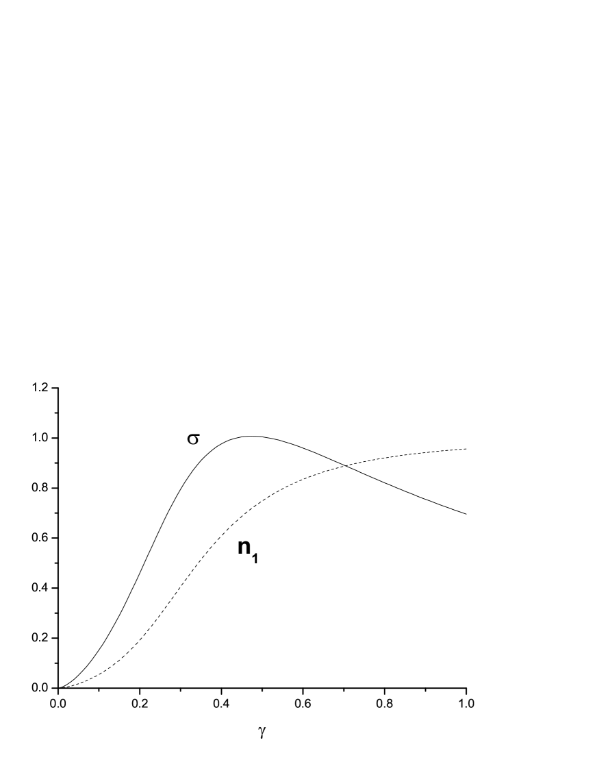
Figure 3: Fraction of uncondensed atoms $n_{1}$ (dashed line) and anomalous fraction $\sigma$ (solid line) as functions of the gas parameter $\gamma$.

For the whole region of $\gamma$, we solve numerically the system of Eqs. (65) to (68), showing the results in Figs. 1,2, and 3.

Figure 1 presents the condensate fraction (66) and this fraction (69) in the Bogolubov approximation. At small $\gamma$, up to $\gamma\approx 0.1$, $n_{0}$ and $n_{B}$ practically coincide with each other. For $\gamma>0.1$, the Bogolubov approximation overestimates the condensate fraction. But $n_{B}=0$ at $\gamma=0.762$, while $n_{0}$ is yet finite, though small. The condensate fraction of a homogeneous Bose gas, at zero temperature, as a function of the gas parameter was calculated by means of the Monte Carlo simulation by Giorgini et al. [36] up to $\gamma\approx 0.5$. For this region of $\gamma$, our $n_{0}$ is in good agreement with the Monte Carlo calculations. Monte Carlo techniques have also been used for studying the condensate fraction of trapped atoms [37–39]. But the latter results cannot be directly compared with $n_{0}$ in a homogeneous gas, since in traps, the condensate fraction is a function of spatial variables as well as of the trap shape [37–41]. What is possible and interesting to compare is the condensate fraction in superfluid ⁴He at zero temperature and our $n_{0}$ at $\gamma\approx 0.6$ corresponding to liquid ⁴He with hard-core interactions. For $\gamma\approx 0.6$, we have $n_{0}\approx 0.15$, which is close to the condensate fraction $n_{0}\approx 0.1$, measured in experiments (as is reviewed in Refs. [3,42]) as well as obtained by Monte Carlo simulations (see review articles [43,44]).

Figure 2 shows the dimensionless sound velocity (62) and its Bogolubov approximation (70). These quantities practically coincide up to $\gamma\approx 0.1$. For $\gamma>0.1$ the Bogolubov form $s_{B}$ underestimates $s$ till $\gamma\approx 0.7$, after which it overestimates the latter.

In Fig. 3, we compare the fraction of uncondensed atoms (67) with the anomalous fraction (68). As is seen, $\sigma>n_{1}$ up to $\gamma\approx 0.7$. The anomalous fraction $\sigma$ becomes substantially smaller than $n_{1}$ only for very large $\gamma\gg 1$. This is in agreement with other calculations [45] confirming that anomalous averages cannot be neglected at low temperatures.

Let us now analyse the ground-state energy

$$E\;\equiv\;<H>+\mu N\qquad(T=0)\;.$$ (77)

According to Eq. (43),

$$<H>\;=\;E_{B}\qquad(T=0)\;.$$

The system chemical potential, defined in Eq. (18), is expressed through the Lagrange multipliers (46) and (47) and the fractions $n_{0}$ and $n_{1}$, which gives

$$\mu=(1+n_{1}+\sigma-2\sigma n_{1})\rho\Phi_{0}\;.$$ (78)

For the dimensionless chemical potential

$$\overline{\mu}\equiv\frac{2m\mu}{\rho^{2/3}}\;,$$ (79)

we get

$$\overline{\mu}=8\pi\gamma(1+n_{1}+\sigma-2\sigma n_{1})\;.$$ (80)

From Eq. (44), we have

$$E_{B}=E_{HFB}+N\int\frac{\varepsilon_{k}-\omega_{k}}{2\rho}\;\frac{d{\bf k}}{(2\pi)^{3}}\;,$$ (81)

where the integral is calculated invoking the dimensional regularization [5], giving

$$\int\frac{\varepsilon_{k}-\omega_{k}}{2\rho}\;\frac{d{\bf k}}{(2\pi)^{3}}=\frac{8(mc)^{5}}{15\pi^{2}m\rho}\;.$$

Equations (34) and (41) yield

$$\frac{E_{HFB}}{N}=\frac{\rho\Phi_{0}}{2}\left(n_{0}^{2}-2n_{1}^{2}-\sigma^{2}\right)-\mu_{0}n_{0}\;.$$ (82)

Summarizing these formulas, we find

$$\frac{E}{N}=\frac{\rho\Phi_{0}}{2}\left(1+n_{1}^{2}-2\sigma n_{1}-\sigma^{2}\right)+\frac{8(mc)^{5}}{15\pi^{2}m\rho}\;.$$ (83)

It is convenient to define the dimensionless ground-state energy

$$E_{0}\equiv\frac{2mE}{\rho^{2/3}N}\;,$$ (84)

for which we obtain

$$E_{0}=4\pi\gamma\left(1+n_{1}^{2}-2\sigma n_{1}-\sigma^{2}+\frac{4s^{5}}{15\pi^{3}\gamma}\right)\;.$$ (85)

This can be compared with the Lee-Huang-Yang approximation [46–48]

$$E_{LHY}=4\pi\gamma\left(1+\frac{128}{15\sqrt{\pi}}\;\gamma^{3/2}\right)\;,$$ (86)

derived for small $\gamma$.

In the limits of asymptotically small and large $\gamma$, the dimensionless chemical potential (80) tends to

$$\overline{\mu}\rightarrow 8\pi\gamma+\frac{256}{3}\;\sqrt{\pi}\;\gamma^{5/2}\qquad(\gamma\rightarrow 0)$$ (87)

and, respectively,

$$\overline{\mu}\rightarrow 16\pi\gamma\qquad(\gamma\rightarrow\infty)\;.$$ (88)

The dimensionless ground-state energy (85) at small $\gamma\ll 1$ possesses the expansion

$$E_{0}\simeq 4\pi\gamma+\frac{512}{15}\;\sqrt{\pi}\;\gamma^{5/2}+\frac{512}{9}\;\gamma^{4}\;,$$ (89)

which reproduces the Lee-Huang-Yang approximation (86) for $\gamma\rightarrow 0$. And for large $\gamma\gg 1$, we find

$$E_{0}\simeq 8\pi\gamma+\frac{6}{5}\left(9\pi^{4}\right)^{1/3}\;-\;\frac{3}{4}\left(3\pi^{5}\right)^{1/3}\gamma^{-1}+\frac{1}{64}\left(3\pi^{8}\right)^{1/3}\gamma^{-4}\;.$$ (90)

Note that expressions (87) and (88) can also be obtained from Eq. (89) and (90) using the relation $\mu=\partial E/\partial N$, valid for $T=0$.

Figure 4 illustrates the behaviour of the ground-state energy (85) and the Lee-Huang-Yang approximation (86). The latter is known to practically coincide with the energy calculated trough the Monte Carlo simulations [36] up to $\gamma\approx 0.4$. As is seen from the figure, our $E_{0}$ is also very close to $E_{LHY}$ in the region $0\leq\gamma<0.4$, but is lower than $E_{LHY}$ for $\gamma>0.4$. Hence, $E_{0}$ well reproduces the available data of Monte Carlo calculations up to $\gamma\approx 0.4$.

5 Conclusion

The notion of representative statistical ensembles is applied to Bose systems with broken global gauge symmetry. A general procedure is described for constructing the grand Hamiltonian for the representative ensemble of an arbitrary equilibrium Bose system. A self-consistent mean-field theory is developed, which is both conserving and gapless. The properties of a uniform Bose gas at zero temperature are studied both analytically and numerically for the gas parameter varying between zero and infinity. Thus, in the frame of the suggested approach, strongly interacting systems can also be considered. For instance, as is known [35,43], some of the properties of superfluid ⁴He can be understood by treating the potential as a hard-core interaction of diameter $a_{s}=2.139\AA$, which, at saturated vapor pressure, corresponds to $\gamma\approx 0.6$. For the latter $\gamma$, we find the condensate fraction $n_{0}$ of order $10\%$, which agrees with the condensate fraction in helium at zero temperature, measured in experiments [42] and found in Monte Carlo simulations [43], being also of order $10\%$. Another application of the developed self-consistent mean-field theory with arbitrary strong interactions could be the description of Bose-Einstein condensation of multiquark clusters in nuclear matter [49,50].

Acknowledgement

One of the authors (V.I.Y.) is grateful for financial support to the German Research Foundation and for discussions to M. Girardeau, R. Graham, and H. Kleinert.

Figure Captions

Fig. 1. Condensate fraction $n_{0}$ (solid line) and its Bogolubov approximation $n_{B}$ (dashed line) as functions of the gas parameter $\gamma$.

Fig. 2. Dimensionless sound velocity $s$ (solid line) and its Bogolubov approximation $s_{B}$ (dashed line) as functions of the gas parameter $\gamma$.

Fig. 3. Fraction of uncondensed atoms $n_{1}$ (dashed line) and anomalous fraction $\sigma$ (solid line) as functions of the gas parameter $\gamma$.

Fig. 4. Dimensionless ground-state energy $E_{0}$ (solid line) and the Lee-Huang-Yang approximation $E_{LHY}$ (dashed line) as functions of the gas parameter $\gamma$.

Figure 1: Condensate fraction $n_{0}$ (solid line) and its Bogolubov approximation $n_{B}$ (dashed line) as functions of the gas parameter $\gamma$.

Figure 2: Dimensionless sound velocity $s$ (solid line) and its Bogolubov approximation $s_{B}$ (dashed line) as functions of the gas parameter $\gamma$.

Figure 4: Dimensionless ground-state energy $E_{0}$ (solid line) and the Lee-Huang-Yang approximation $E_{LHY}$ (dashed line) as functions of the gas parameter $\gamma$.

References

- [1] A.S. Parkins and D.F. Walls, Phys. Rep. 303, 1 (1998).
- [2] F. Dalfovo, S. Giorgini, L.P. Pitaevskii, and S. Stringari, Rev. Mod. Phys. 71, 463 (1999).
- [3] P.W. Courteille, V.S. Bagnato and V.I. Yukalov, Laser Phys. 11, 659 (2001).
- [4] A.L. Fetter, J. Low Temp. Phys. 129, 263 (2002).
- [5] J.O. Andersen, Rev. Mod. Phys. 76, 599 (2004).
- [6] K. Bongs and K. Sengstock, Rep. Prog. Phys. 67, 907 (2004).
- [7] V.I. Yukalov, Laser Phys. Lett. 1, 435 (2004).
- [8] N.N. Bogolubov, J. Phys. (Moscow) 11, 23 (1947).
- [9] N.N. Bogolubov, Moscow Univ. Phys. Bull. 7, 43 (1947).
- [10] E. Timmermans, P. Tommasini, M. Hussein, and A. Kerman, Phys. Rep. 315, 199 (1999).
- [11] R.A. Duine and H.T.C. Stoof, Phys. Rep. 396, 115 (2004).
- [12] P.C. Hohenberg and P.C. Martin, Ann. Phys. 34, 291 (1965).
- [13] V.I. Yukalov, Phys. Rev. E 72, 066119 (2005).
- [14] V.I. Yukalov and H. Kleinert, Phys. Rev. A 73, 063612 (2006).
- [15] F.A. Berezin, Method of Second Quantization (Academic, New York, 1966).
- [16] V.I. Yukalov, Statistical Green’s Functions (Queen’s University, Kingston, 1998).
- [17] N.N. Bogolubov, Lectures on Quantum Statistics (Gordon and Breach, New York, 1967), Vol. 1.
- [18] N.N. Bogolubov, Lectures on Quantum Statistics (Gordon and Breach, New York, 1970), Vol. 2.
- [19] V.I. Yukalov, Laser Phys. 16, 511 (2006).
- [20] J.W. Gibbs, Collected Works (Longmans, New York, 1954), Vol. 2.
- [21] V.I. Yukalov, Phys. Rep. 208, 395 (1991).
- [22] N.M. Hugenholtz and D. Pines, Phys. Rev. 116, 489 (1959).
- [23] J. Gavoret and P. Nozières, Ann. Phys. (N.Y.) 28, 349 (1964).
- [24] M. Girardeau and R. Arnowitt, Phys. Rev. 113, 755 (1959).
- [25] M. Girardeau, J. Math. Phys. 3, 131 (1962).
- [26] M. Girardeau, Phys. Rev. 115, 1090 (1959).
- [27] F. Takano, Phys. Rev. 123, 699 (1961).
- [28] V.I. Yukalov, Laser Phys. Lett. 3, 406 (2006).
- [29] P.O. Löwdin, Phys. Rev. 97, 1474 (1955).
- [30] A.J. Coleman and V.I. Yukalov, Reduced Density Matrices (Springer, Berlin, 2000).
- [31] N.N. Bogolubov and N.N. Bogolubov Jr., Introduction to Quantum Statistical Mechanics (Gordon and Breach, Lausanne, 1994).
- [32] H. Kleinert, Path Integrals (World Scientific, Singapore, 2004).
- [33] K. Xu, Y. Liu, D.E. Miller, J.K. Chim, W. Setiawan, and W. Ketterle, Phys. Rev. Lett. 96, 180405 (2006).
- [34] M.H. Kalos, Phys. Rev. A 2, 250 (1970).
- [35] M.H. Kalos, D. Levesque, and I. Verlet, Phys. Rev. A 9, 2178 (1974).
- [36] S. Giorgini, J. Boronat, and J. Casulleras, Phys. Rev. A 60, 5129 (1999).
- [37] J.L. DuBois and H.R. Glyde, Phys. Rev. A 63, 023602 (2001).
- [38] J.L. DuBois and H.R. Glyde, Phys. Rev. A 68, 033602 (2003).
- [39] W. Purwanto and S. Zhang, Phys. Rev. A 72, 053610 (2005).
- [40] K. Nho and D. Blume, Phys. Rev. Lett. 95, 193601 (2005).
- [41] K. Nho and D.P. Landau, Phys. Rev. A 73, 033606 (2006).
- [42] F.W. Wirth and R.B. Hallock, Phys. Rev. B 35, 34 (1987).
- [43] D.M. Ceperley, Rev. Mod. Phys. 67, 279 (1995).
- [44] M. Boninsegni, N.V. Prokofiev, and B.V. Svistunov, Phys. Rev. E 74, 036701 (2006).
- [45] V.I. Yukalov and E.P. Yukalova, Laser Phys. Lett. 2, 506 (2005).
- [46] T.D. Lee and C.N. Yang, Phys. Rev. 105, 1119 (1957).
- [47] T.D. Lee, K. Huang, and C.N. Yang, Phys. Rev. 106, 1135 (1957).
- [48] T.D. Lee and C.N. Yang, Phys. Rev. 112, 1419 (1958).
- [49] V.I. Yukalov and E.P. Yukalova, Phys. Part. Nucl. 28, 37 (1997).
- [50] A. Faessler, A.J. Buchmann, M.I. Krivoruchenko, and B.V. Martemyanov, Phys. Lett. B 391, 255 (1997).