Probing quantum-mechanical level repulsion in disordered systems by means of time-resolved selectively-excited resonance fluorescence

Abstract

We argue that the time-resolved spectrum of selectively-excited resonance fluorescence at low temperature provides a tool for probing the quantum-mechanical level repulsion in the Lifshits tail of the electronic density of states in a wide variety of disordered materials. The technique, based on detecting the fast growth of a fluorescence peak that is red-shifted relative to the excitation frequency, is demonstrated explicitly by simulations on linear Frenkel exciton chains.

Anderson localization is a key concept in understanding the transport properties and optical dynamics of quasiparticles in disordered systems in general Abrahams79 ; Kramer93 ; Mirlin00 and in a large variety of low-dimensional materials in particular. Examples of current interest are conjugated polymers Hadzii99 , molecular J-aggregates Kobayashi96 ; Bednarz03 , semiconductor quantum-wells Alessi00 ; Klochikhin04 and quantum wires Feltrin04a , as well as biological antenna complexes vanAmerongen00 ; Cheng06 . Localization results in the appearance of a Lifshits tail in the density of states (DOS) below the bare quasiparticle band Lifshits88 ; Chernyak99 . At low temperature, the states in the tail determine the system’s transport and optical properties. Of particular importance for the dynamics and the physical properties is the spatial overlap between these states. Two situations can be distinguished: states that do not overlap can be infinitesimally close in energy, while states that do overlap undergo quantum-mechanical level repulsion. Interestingly, this repulsion does not manifest itself in the overall level statistics, which, due to the localization, is of Poisson nature. The local Wigner-Dyson statistics, caused by the repulsion, turns out to be hidden under the global distribution of energies Malyshev01a . Still, due to the characteristic energy scale associated with the level repulsion, this phenomenon does affect global properties, such as transport Malyshev03 . Moreover, observing changes in the level statistics allows one to detect the localization-delocalization transition or mobility edges Mirlin00 .

Thus, it is of general interest to have experimental probes for the level statistics in disordered systems. Recently, it has been shown that near-field spectroscopy Intonti01 ; Feltrin04b and time-resolved resonant Rayleigh scattering Haacke01 may be used to uncover the statistics of localized Wannier excitons in disordered quantum wells Intonti01 and wires Feltrin04b . In this Letter, we argue that low-temperature time-resolved selectively excited fluorescence from the Lifshits tail provides an alternative tool for probing the level repulsion. This method is based on the fact that downward relaxation between spatially overlapping states dominates the early-time rise of a fluorescence peak that is red-shifted relative to the excitation frequency. The red shift is related to the level repulsion. We will demonstrate this by simulations on a one-dimensional (1D) Frenkel exciton model with on-site disorder. The key ingredients of the model – level repulsion and scattering rates proportional to the phonon spectral density times the overlap integral of the site probabilities of the two exciton states involved Bednarz03 – are also characteristic for Wannier exciton systems Alessi00 ; Klochikhin04 ; Feltrin04a ; Shimizu98 . Hence, the method has a wide range of applicability.

Our model consists of an open chain of $N$ optically active two-level units (monomers) with parallel transition dipoles, coupled to each other by dipole-dipole interactions. The chain’s optical excitations are Frenkel excitons described by a Hamiltonian matrix whose diagonal elements are the monomer excitation energies, $H_{nn}=\varepsilon_{n}$, which are random uncorrelated Gaussian variables with zero mean and standard deviation $\Delta$ (i.e., $\langle\varepsilon_{n}\rangle=0$ and $\langle\varepsilon_{n}\varepsilon_{m}\rangle=\Delta^{2}\delta_{nm}$, with $\langle\ldots\rangle$ denoting the average over the disorder realizations). The off-diagonal matrix elements are non-random dipole-dipole interactions: $H_{nm}=-J/|n-m|^{3}$   $(J_{nn}\equiv 0)$, with $J>0$ representing the magnitude of the nearest-neighbor coupling. The exciton eigenenergies $E_{\nu}$ and eigenfunctions $\varphi_{\nu n}$ follow from diagonalizing $H_{nm}$.

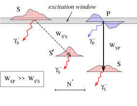
Figure 1: Cartoon of the local DOS tail states, illustrating the possible channels of the exciton relaxation at zero temperature after excitation within a narrow window. The solid (dashed) arrow shows the intra (inter) segment relaxation with the rate $W_{\mathrm{SP}}$ ($W_{\mathrm{S^{\prime}S}}$), while the wavy arrows denote the radiative decay with the typical rate $\gamma^{*}_{\mathrm{S}}=\gamma_{0}N^{*}$ and $\gamma^{*}_{\mathrm{P}}\approx 0.1\gamma_{0}N^{*}$ ($N^{*}$ is the typical segment length).

The states in the Lifshits tail, which dominate the optical absorption of the disordered chain, are localized on segments of typical size $N^{*}$. Some of these states can be joined in local exciton manifolds of a few states that are similar to the eigenstates of an ideal chain of size equal to the segment length Malyshev01a ; footnote1 . The states in a local manifold undergo level repulsion, while between different segments energy separations may be arbitrarily small. Because the variation of exciton energies over different segments is larger than the level repulsion within segments Malyshev01a , the latter remains hidden in techniques that probe global averages like, e.g., the absorption spectrum.

The typical situation is illustrated in Fig. 1. The two states to the right form a local manifold, with the lower state having no node and collecting most of the oscillator strength of the monomers within the segment. We will refer to this as an S type state. The higher state has one node (P type) and has a much smaller (but nonzero) oscillator strength; thus, it can be photo-excited but its radiative decay is slow compared to that of the S state. The probability overlap between the two states, measured by the integral $I_{\mu\nu}=\sum_{n=1}^{N}\varphi_{\mu n}^{2}\varphi_{\nu n}^{2}$, is on the order of $1/N_{\mathrm{seg}}$, with $N_{\mathrm{seg}}\sim N^{*}$ the segment (localization) size. The other two states in Fig. 1 are the lowest (S type) states of other localization segments. For linear systems, the overlap between states of adjacent segments typically is two orders of magnitude smaller than the overlap within a manifold Malyshev01a ; for distant segments the overlap is even much smaller. These overlap properties play a crucial role in the intraband exciton relaxation.

To describe this relaxation, we use the Pauli master equation for the populations $P_{\nu}$ of the exciton states:

$${\dot{P}}_{\nu}=R_{\nu}F_{\nu}-\gamma_{\nu}P_{\nu}+\sum_{\mu=1}^{N}(W_{\nu\mu}P_{\mu}-W_{\mu\nu}P_{\nu})\ ,$$ (1)

where $R_{\nu}$ is a source term, specified below, $F_{\nu}=(\sum_{n=1}^{N}\varphi_{\nu n})^{2}$ is the dimensionless oscillator strength of the $\nu$th exciton state, $\gamma_{\nu}=\gamma_{0}F_{\nu}$ is its spontaneous emission rate ($\gamma_{0}$ being the spontaneous emission constant of a monomer), and $W_{\mu\nu}$ is the scattering rate from the exciton state $|\nu\rangle$ to the state $|\mu\rangle$, which results from weak exciton-vibration coupling. The latter may be obtained through Fermi’s golden rule Bednarz03 : $W_{\mu\nu}=I_{\mu\nu}\;S(|\omega_{\mu\nu}|)\;G(\omega_{\mu\nu})$, where $I_{\mu\nu}$ is the overlap integral defined above and $S(|\omega_{\mu\nu}|)$ is the phonon spectral density at the energy $\omega_{\mu\nu}=E_{\mu}-E_{\nu}$. Furthermore, $G(\omega)=n(\omega)$ if $\omega>0$ and $G(\omega)=1+n(-\omega)$ if $\omega<0$, with $n(\omega)=[\exp(\omega/T)-1]^{-1}$, the mean thermal occupation number of a phonon mode of energy $\omega$ ($\hbar=k_{B}=1$).

We consider an experiment in which a short narrow-band laser pulse is used to selectively excite states in a small part of the absorption band and set $R_{\nu}(t)=R_{0}\delta(t)\delta(E_{l}-E_{\nu})$ with $E_{l}$ being the laser frequency. We are interested in the time-resolved fluorescence spectrum at low temperature ($T=0$). The spectrum is given by

$$I(E,t)=\frac{1}{N}\Big{\langle}\sum_{\nu=1}^{N}\gamma_{\nu}\,P_{\nu}(t)\>\delta(E-E_{\nu})\Big{\rangle}\ .$$ (2)

At $T=0$, only states with $E_{\nu}\leq E_{l}$ are relevant. Quite generally, the spectrum consists of a narrow resonant peak, resulting from fluorescence from initially excited states and a red-shifted broader feature, arising from states that are populated by downward relaxation from the initially excited ones.

If the laser frequency lies in the main part of the absorption band, not too far in the blue wing, the initially excited states are either of the S or of P type. Excitation of higher excited states, which extend over various segments, may be neglected. Both S and P states contribute to the narrow resonant fluorescence, with most of the intensity coming from the S type states, because they carry more oscillator strength. On the other hand, the P type states have a much higher probability to relax to their S partner before they decay radiatively. The S type states can only relax to states of other segments, which is a slow process as compared to the intra-manifold relaxation ($W_{\mathrm{S}{\mathrm{P}}}\gg W_{\mathrm{S}^{\prime}{\mathrm{S}}}$). Therefore, at times $t<1/W_{\mathrm{S}{\mathrm{P}}}$, any red-shifted fluorescence comes from S type states that have been excited via intra-segment relaxation from P type ones. Thus, the shape and position of the red-shifted fluorescence band reflects the level repulsion, i.e., its intensity tends to zero when approaching the laser frequency. At longer times, this repulsive gap may be partially filled due to inter-segment hops.

We now analyze in more detail the early-time shape of the red-shifted band $I_{\mathrm{red}}(E,t)$. For $t\ll 1/\gamma^{*}_{\mathrm{P}}+1/W_{\mathrm{S}{\mathrm{P}}}$, one iteration of the master equation gives

$$I_{\mathrm{red}}(E,t) = \frac{R_{0}t}{N}\Big{\langle}\sum_{\mu,\nu}\gamma_{\nu}\,W_{\nu\mu}F_{\mu}\delta(E_{\mu}-E_{l})\>\delta(E-E_{\nu})\Big{\rangle}$$ (3)

$$= \frac{R_{0}t}{N}S(E_{l}-E)\Big{\langle}\sum_{\mu,\nu}\gamma_{\nu}\,I_{\nu\mu}F_{\mu}\,$$

$$\times \delta(E_{\mu}-E_{l})\>\delta(E-E_{\nu})\Big{\rangle}\ ,$$

where the sum is restricted to states which occur in SP doublets, as described above. Thus, $\mu$ ($\nu$) in the sum label P (S) type states. Because $I_{\mathrm{SP}}\sim 1/N_{\mathrm{seg}}$, while the lower state in each segment has a superradiant decay rate $\gamma_{\mathrm{S}}\approx\gamma_{0}N_{\mathrm{seg}}$, we have $\gamma_{\nu}\,I_{\nu\mu}=a\gamma_{0}$, with $a$ being a constant of the order unity. If we now replace $F_{\mu}$ by the average oscillator strength $F_{\mathrm{P}}(E_{l})$ for P type states at the energy $E_{l}$, we arrive at

$$I_{\mathrm{red}}(E,t)=\frac{a\gamma_{0}R_{0}t}{N}\>F_{\mathrm{P}}(E_{l})\>S(E_{l}-E)\>P_{\mathrm{SP}}(E_{l},E)\ .$$ (4)

Here, $P_{\mathrm{SP}}(E_{l},E)=\big{\langle}\sum_{\mu,\nu}\delta(E_{\mu}-E_{l})\>\delta(E-E_{\nu})\big{\rangle}$ is the probability distribution for the energy of an S state under the condition that the same localization segment contains a P state at the energy $E_{l}$. This result shows that the early-time lineshape is the product of the phonon spectral density and the conditional spacing distribution, thus containing detailed information about the repulsive level statistics.

To confirm the above analytical result, we have performed numerical simulations of the spectrum Eq. (2) for 1D Frenkel chains of length $N=1000$ at $T=0$. In all calculations we considered system parameters that are appropriate for linear aggregates of the dye pseudoisocyanine (PIC) with counter ion F^-: $\gamma_{0}=2.7\times 10^{8}\,{\mathrm{s}}^{-1}=1.5\times 10^{-5}J$, $J=600$ cm^-1, and $\Delta=0.25\,J$, giving a typical localization size $N^{*}=28$. For the spectral density we used the Debye model: $S(\omega)=W_{0}(\omega/J)^{3}$, with $W_{0}=15.9J$. This set of parameters has been used successfully to analyze and fit experiments on aggregates of PIC-F Bednarz03 . As at $T=0$ only states below the excitation energy are relevant, we used the Lanczos method to calculate the subset of only these eigenstates. The fluorescence spectra were obtained after averaging over $10^{5}$ realizations of the on-site energies.

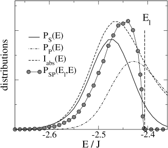
Figure 2: Calculated energy distributions of S type states (solid curve), P type states (dash-dotted curve), absorption spectrum (dashed curve), and the conditional probability $P_{\mathrm{SP}}(E_{l},E)$ (filled circles).

First, we analyzed numerically various statistical properties of the exciton levels. The results are summarized in Fig. 2. Shown are the distribution of energies of the S and P type states, $P_{\mathrm{S}}(E)$ and $P_{\mathrm{P}}(E)$, respectively, the absorption spectrum, $I_{\mathrm{abs}}(E)$, and the conditional probability $P_{\mathrm{SP}}(E_{l},E)$, with $E_{l}=-2.41J$. The selection of doublets of S and P type states was done according to the method described in Ref. Malyshev01a,  footnote2 . Clearly, the low-energy half of the absorption peak is dominated by S type states, while the high-energy wing contains also important contributions from P type states. Both distributions overlap, which is the reason that the local energy structure is not seen in the absorption peak. The conditional probability clearly demonstrates the level repulsion, as it drops to zero at $E=E_{l}$. In our simulations the laser energy $E_{l}$ was chosen such that it pumps primarily P type states.

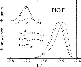
Figure 3: Zero-temperature time-resolved fluorescence spectra at different instants. The intensities of the red-shifted bands are normalized to the same peak value. The inset shows the unnormalized spectra.

Figure 3 presents our numerical results for the time-resolved fluorescence spectrum after selective excitation within a window [$-2.415J,-2.405J$]. Indeed, the spectrum reveals a sharp peak at the excitation energy and a clearly separated red-shifted (R) band, indicative of level repulsion. The kinetics of this band can be understood from estimates of the radiative decay and relaxation rates. Typically, $\gamma_{\mathrm{S}}^{*}=\gamma_{0}N^{*}\approx 10\gamma_{\mathrm{P}}^{*}\approx 4\times 10^{-4}J$, while $W_{\mathrm{SP}}\approx 10^{2}W_{\mathrm{S^{\prime}S}}\approx W_{0}(\Delta^{*}/J)^{3}I_{\mathrm{SP}}\approx 6\times 10^{-5}J$. Here we used the typical energy separation $\Delta^{*}=\Delta/\sqrt{N^{*}}$ and $I_{\mathrm{SP}}\approx 1/N^{*}$ ($N^{*}=28$). Thus, $W_{\mathrm{S^{\prime}S}}\ll\gamma_{\mathrm{P}}^{*}<W_{\mathrm{SP}}\ll\gamma_{\mathrm{S}}^{*}$, implying that inter-segment hops are irrelevant on the radiative time scale. As a consequence, the observed blue-shift of the R band upon increasing time, cannot be the result of filling the repulsive gap by such hops. Instead, this kinetics results from the fact that the oscillator strength per state peaks at lower energies than the absorption maximum Bednarz03 . Thus, the higher-energy states in the R band decay slower, causing the blue-shift.

Finally, Fig. 4 displays the numerically obtained early-time fluorescence spectra, for $t=0.01W_{\mathrm{SP}}^{-1}$, $0.02W_{\mathrm{SP}}^{-1}$, and $0.03W_{\mathrm{SP}}^{-1}$. The spectra are normalized by dividing by the time $t$ at which they were taken. Clearly, the resulting curves cannot be distinguished. Moreover, they agree almost perfectly with the function $(E_{l}-E)^{3}P_{\mathrm{SP}}(E_{l},E)$, plotted as open circles. This confirms the analytical expression (4). Without showing explicit results, we note that the same quality of agreement has been found for other model parameters and spectral densities.

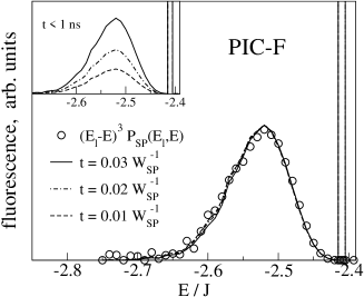
Figure 4: Simulated fluorescence spectra at three early instances of time, normalized by dividing by $t$ and compared to the function $(E_{l}-E)^{3}P_{\mathrm{SP}}(E_{l},E)$ (open circles). The inset shows the unnormalized spectra.

In summary, we have shown that time-resolved selective excitation of fluorescence in the Lifshits tail of low-temperature disordered systems, yields a probe for the quantum level repulsion and local level statistics. Shortly after the laser pulse, the shape of the red-shifted fluorescence band arising in this technique is the product of the level spacing distribution within localization segments and the phonon spectral density. To extract the spacing distribution, the spectral density must be measured. The widely adapted scheme for this also employs low-temperature selectively excited fluorescence, but under steady-state conditions. It is assumed that the red-shifted band directly reflects the phonon spectral density Renger02 . However, for multichromophore systems with a fast intra-band relaxation, this approach is not appropriate, because a relaxation-induced red-shifted feature, which also arises under steady-state conditions Bednarz05 , is superimposed with the phonon side-band. The two contributions may be separated by measuring the time-dependent spectrum. Thus, time resolution is an essential aspect of the scheme proposed. Of course, the relation between pulse width (selective excitation) and duration (time-resolution) limits application of our approach to systems for which the absorption band is wide compared to the intraband relaxation rate. For the example considered here, this criterion is easily met.

To conclude we stress that our method has a wider applicability than the 1D Frenkel exciton system we modeled. The reason is that the key ingredients – the nature of the states in the Lifshits tail and the importance of spatial overlap for their phonon-induced relaxation – are shared by a large variety of systems Alessi00 ; Klochikhin04 ; Feltrin04a ; Bednarz03 ; Shimizu98 .

This work was supported by the programs Ramón y Cajal (Ministerio de Ciencia y Tecnología de España) and NanoNed (Dutch Ministry of Economic Affairs).

References

- (1) E. Abrahams et al., Phys. Rev. Lett. 42, 673 (1979).
- (2) B. Kramer and A. MacKinnon, Rep. Prog. Phys. 56, 1469 (1993).
- (3) A. D. Mirlin, Phys. Rep. 326, 259 (2000).
- (4) See, e.g., ”Semiconducting Polymers - Chemistry, Physics, and Engineering”, eds. G. Hadziioannou and P. van Hutten (VCH, Weinheim, 1999).
- (5) J-aggregates, ed. T. Kobayashi (World Scientific, Singapore, 1996).
- (6) M. Bednarz, V. A. Malyshev, and J. Knoester, Phys. Rev. Lett. 91, 217401 (2003); J. Chem. Phys. 120, 3827 (2004); D. J. Heijs, V. A. Malyshev, and J. Knoester, Phys. Rev. Lett. 95, 177402 (2005).
- (7) M. Grassi Alessi et al., Phys. Rev. B 61, 10985 (2000).
- (8) A. Klochikhin et al., Phys. Rev. B 69, 085308 (2004).
- (9) A. Feltrin et al. Phys. Rev. B 69, 233309 (2004).
- (10) H. van Amerongen, L. Valkunas and R. van Grondelle, Photosynthetic Excitons (World Scientific, Singapore, 2000).
- (11) Y. C. Cheng and R. J. Silbey, Phys. Rev. Lett. 96, 028103 (2006).
- (12) I. M. Lifshits, Sov. Phys. JETP 26, 462 (1968).
- (13) V. Chernyak et al., J. Phys. Chem. A 103, 10294 (1999).
- (14) A. V. Malyshev and V. A. Malyshev, Phys. Rev. B 63, 195111 (2001).
- (15) A. V. Malyshev, V. A. Malyshev and F. Domínguez-Adame, J. Phys. Chem. B 107, 4418 (2003).
- (16) F. Intonti et al., Phys. Rev. Lett. 87, 76801 (2001).
- (17) A. Feltrin et al, Phys. Rev. B 69, 205321 (2004).
- (18) S. Haacke, Rep. Prog. Phys. 64, 737 (2001).
- (19) M. Shimizu et al., Phys. Rev. B 58, 5032 (1998).
- (20) The segments on which such local manifolds are found usually do not correspond to the optimal disorder fluctuations. The latter describe states that occur deeper in the Lifshits tail (see, e.g., Ref. Chernyak99, ), localized as singlets, without higher-energy partners on the same segment.
- (21) To select the SP doublets, we used and in the selection rules elaborated in Ref. Malyshev01a, .
- (22) See, e.g., T. Renger and R. A. Marcus, J. Chem. Phys. 116, 9997 (2002), and references therein.
- (23) M. Bednarz, V. A. Malyshev, and J. Knoester, J. Lumin. 112, 411 (2005); M. Bednarz and P. Reineker, J. Lumin. 119-120, 482 (2006).