Structure factor and dynamics of the helix-coil transition

Abstract

Thermodynamical properties of the helix-coil transition were successfully described in the past by the model of Lifson, Poland and Sheraga. Here we compute the corresponding structure factor and show that it possesses a universal scaling behavior near the transition point, even when the transition is of first order. Moreover, we introduce a dynamical version of this model, that we solve numerically. A Langevin equation is also proposed to describe the dynamics of the density of hydrogen bonds. Analytical solution of this equation shows dynamical scaling near the critical temperature and predicts a gelation phenomenon above the critical temperature. In the case when comparison of the two dynamical approaches is possible, the predictions of our phenomenological theory agree with the results of the Monte Carlo simulations.

PACS: 87.10.Gg, 64.60.Fr, 64.60.Ht

I Introduction

Ever since the discovery of the helicoidal structure of DNA under the usual conditions, the phenomenon of its transformation to a coil under heating has been studied and described as an equilibrium phase transition. Basic works by Lifson and subsequently by Poland and Sheraga led to a model (LPS) considered today standard L ; PS . The model is one-dimensional and shows a phase transition only because the interactions are long-ranged. A more realistic description of the two strands moving and interacting in three dimensional space has also been proposed and studied numerically Caruso; Carlon ; Baiesi ; BaKa . A model of LPS–type was shown to be able to consistently fit all relevant simulation results Schafer . More recently, some authors have proposed a new mechanism which yields an abrupt first–order phase transition Peliti ; Blossey , at variance with the previous theoretical considerations in favor of a continuous one. On the experimental side the situation is still far from conclusive. Previous measurements indicated the presence of a sharp jump in the fraction of bound base pairs Wartell ; Blake . More recently, the results reported in Zocchi have been interpreted as an indication of a weakly continuous phase transition.

It seems, however, that little is known about the dynamics of this denaturation transition. We can mention the contributions based on a mechanical approach Bishop2 ; Theodora and on a Langevin description of the two DNA–strands as polymers in continuous space Nelson .

In this paper we investigate the original LPS model while considering the exponent $\alpha$ as a free parameter. For what concerns the equilibrium properties we compute the structure factor and find that near the critical point it exhibits universal scaling behavior, which depends only on $\alpha$. Moreover, we also look at the transition from a dynamical point of view. We do it in two ways: first we describe this dynamics by a master equation such that the equilibrium state is chosen to be the one of the LPS model. Secondly, we introduce a Langevin type equation for the order parameter which is the density of hydrogen bonds. The analysis of the solution of this equation reveals a critical slowing-down, the relaxation time diverging at the critical point with a power law still depending on $\alpha$. In the absence of noise, we find that above the critical temperature a gelation phenomenon occurs, namely the density of H-bonds approaches zero in a finite time. With the addition of noise we obtain also the analytic expression for the power–spectrum of the density of H-bonds. Finally, we compare the two descriptions and find that the dynamics of the order parameter derived from the master equation and from the Langevin equations essentially agree.

The following three sections are devoted to a study of equilibrium properties. In Section II we summarize the basics of the LPS model. Formulas for the free energy and the pressure are given here, as well as scaling formulas for the density in the vicinity of the phase transition. Section III contains the computation of the one- and two-point correlation functions for finite systems and in the thermodynamic limit. Our results for the structure factor are presented in Section IV. Results on the dynamics are collected in Sections V and VI. In Section V we describe the microscopic dynamics realized numerically in this work. The equation for the order parameter and its analysis both with and without noise is given in Section VI, where we also compare the results of the two dynamical approaches. The paper ends with a Summary.

II The LPS model

Let 0 and 1 denote respectively a broken or existing H-bond at a given site. Then, a configuration of the double-strand of DNA of length $N$ is represented by a sequence ${\bf n}=\{n_{x}\}_{x=1}^{N}$ where $n_{x}=0$ or 1. In ${\bf n}$ there are alternating maximal connected subsequences (intervals) of 1 and 0, respectively. A weight $a(j)>0$ or $b(j)>0$ is associated to an interval of length $j$ of 1 or 0, respectively. If the lengths of the intervals of ${\bf n}$ are $l_{i}$ and $m_{j}$ then the weight of ${\bf n}$ is

$$e^{-V({\bf n})}=\prod_{i}a(l_{i})\prod_{j}b(m_{j})\ .$$ (2.1)

As usual, thermal equilibrium can be discussed in the canonical or in the grand-canonical ensemble. In the first case the description is restricted to configurations with the total number of H-bonds, $n=\sum_{x}n_{x}$, fixed. In the second case all configurations compatible with the boundary condition are considered but an activity $e^{\beta\mu}$ is introduced. The chemical potential $\mu$ is the energy needed to break a H-bond. The canonical partition function is

$$Q_{N,n}=\sum_{{\bf n}:\sum_{x}n_{x}=n}e^{-V({\bf n})}$$ (2.2)

and the grand-canonical partition function is

$$Q_{N}(\beta\mu)=\sum_{n}Q_{N,n}e^{n\beta\mu}=\sum_{{\bf n}}e^{-U({\bf n})}$$ (2.3)

where $U({\bf n})=V({\bf n})-\beta\mu\sum_{x}n_{x}$. Alternately, $e^{-U({\bf n})}$ is obtained from $e^{-V({\bf n})}$ by replacing each factor $a(l)$ by $a(l)e^{l\beta\mu}$. The free energy $f$ and the pressure $p$ are respectively given by

$$\beta f=-\lim_{\begin{array}[]{cc}N\to\infty\\ n/N\to\rho\end{array}}\frac{1}{N}\ln Q_{N,n}$$ (2.4)

and

$$\beta p=\lim_{N\to\infty}\frac{1}{N}\ln Q_{N}(\beta\mu).$$ (2.5)

The temperature does not appear explicitly in the canonical partition function, therefore $\beta f$ is independent of $\beta$ and $\beta p$ depends on it through $\epsilon=\beta\mu$. The free energy and the pressure are Legendre transforms of each other,

$$\beta p(\epsilon)=\sup_{\rho}\{\epsilon\rho-\beta f(\rho)\}\equiv\epsilon\rho_{\epsilon}-\beta f(\rho_{\epsilon})$$ (2.6)

and

$$\beta f(\rho)=\sup_{\epsilon}\{\epsilon\rho-\beta p(\epsilon)\}\equiv\epsilon_{\rho}\rho-\beta p(\epsilon_{\rho})\ .$$ (2.7)

Here $\rho$ is the density of 1 (H-bonds), and $\rho_{\epsilon}$ and $\epsilon_{\rho}$ are the respective values at which the suprema are attained.

The partition functions depend on the boundary conditions imposed on the system. Typical choices are the free and the periodic conditions, or fixed 0 or 1 on the boundary sites. For example, with the choice $0\ldots 1$ or $1\ldots 0$,

$$Q_{N,n}=\sum_{k\geq 1}A_{k}(n)B_{k}(N-n)$$ (2.8)

where

$$A_{k}(n)=\sum_{l_{1}\geq 1}\cdots\sum_{l_{k}\geq 1}\prod_{i=1}^{k}a(l_{i})\delta_{n,\sum l_{i}}$$ (2.9)

and

$$B_{k}(n)=\sum_{m_{1}\geq 1}\cdots\sum_{m_{k}\geq 1}\prod_{i=1}^{k}b(m_{i})\delta_{n,\sum m_{i}}.$$ (2.10)

$A_{k}(n)=B_{k}(n)=0$ if $n\leq 0$ or $k>n$, therefore $Q_{N,n}=0$ for $n\geq N$. One can show that in the thermodynamic limit the free energy and the pressure do not depend on the boundary condition. Below we give these quantities in the case of the simplest model (the LPS model in a strict sense) obtained by choosing

$$a(l)=a\qquad b(l)=bu^{l}l^{-\alpha}$$ (2.11)

where $u,\alpha>1$ and $a,b>0$ . With the notations $c=ab$,

$$\zeta_{\alpha}(x)=\sum_{l=1}^{\infty}l^{-\alpha}e^{-lx}\qquad(x\geq 0)$$ (2.12)

and

$$\epsilon_{c}=\ln u-\ln[1+c\,\zeta_{\alpha}(0)],$$ (2.13)

one obtains

$$\beta p=\ln u+\Theta(\epsilon-\epsilon_{c})x(\epsilon)$$ (2.14)

where $\Theta$ is the Heaviside function and, for $\epsilon>\epsilon_{c}$, $x(\epsilon)$ is the unique solution of the equation

$$ue^{x-\epsilon}=1+c\,\zeta_{\alpha}(x)\ .$$ (2.15)

Thus, $x(\epsilon_{c})=0$ and $x(\epsilon)$ is monotone increasing with $\epsilon$. For $\epsilon<\epsilon_{c}$, $\beta p$ takes on its minimum value, $\ln u$. Comparison with (2.4), (2.5) and (2.11) shows that the corresponding density and free energy are $\rho_{\epsilon}\equiv 0$ and $f(\rho_{\epsilon})\equiv-\ln u$. Legendre transformation yields $f(\rho)$ for all $\rho$. With $\rho_{c}\equiv\rho_{\epsilon_{c}}$,

$$\beta f(\rho)=\left\{\begin{array}[]{ll}\!-\ln u+\epsilon_{c}\rho,&\rho\leq\rho_{c}\\ \!-\ln u-y+\rho\!\left(y+\ln\frac{u}{1+c\,\zeta_{\alpha}(y)}\right),&\rho\geq\rho_{c}\end{array}\right.$$ (2.16)

where $y=y(\rho)$ is the solution of the equation

$$1+\frac{c\,\zeta_{\alpha-1}(y)}{1+c\,\zeta_{\alpha}(y)}=\rho^{-1}.$$ (2.17)

In fact, $y(\rho)=x(\epsilon_{\rho})$; $y(\rho)$ is defined for $\rho_{c}\leq\rho\leq 1$ and is monotone increasing, $y(\rho_{c})=0$ and $y(1)=\infty$. Therefore, $f(\rho)$ is monotone increasing from $f(0)=-\beta^{-1}\ln u$ to $f(1)=0$; as the Legendre transform of the convex $p(\epsilon)$, $f(\rho)$ is also convex. Substituting $y=0$ into (2.17) yields

$$\rho_{c}=\frac{1+c\,\zeta_{\alpha}(0)}{1+c\,[\zeta_{\alpha-1}(0)+\zeta_{\alpha}(0)]}.$$ (2.18)

This shows that $\rho_{c}=0$ if $\alpha\leq 2$ and $\rho_{c}>0$ if $\alpha>2$. The first case corresponds to a continuous phase transition with the order parameter $\rho_{\epsilon}$ vanishing continuously as $\epsilon$ approaches $\epsilon_{c}$ from above. In the second case the transition is of first order: $\rho_{\epsilon}$ decreases continuously to $\rho_{c}$ as $\epsilon$ decreases to $\epsilon_{c}$ and jumps to zero below $\epsilon_{c}$. Computation of $\rho^{\prime}_{\epsilon}={\,\rm d}\rho_{\epsilon}/{\,\rm d}\epsilon$ from Eq. (2.17) shows that $\rho^{\prime}_{\epsilon_{c}+0}=\infty$ if $\alpha\leq 3$ (while it is finite for $\alpha>3$). The type of divergence can be extracted from the asymptotic forms

$$\rho_{\epsilon}\sim(\epsilon-\epsilon_{c})^{2-\alpha}\quad{\rm if\ }1<\alpha<2$$

$$\rho_{\epsilon}-\rho_{c}\sim\left\{\begin{array}[]{cl}(\epsilon-\epsilon_{c})^{\alpha-2}&{\rm if\ }2<\alpha<3\\ |\ln(\epsilon-\epsilon_{c})|^{-1}&{\rm if\ }\alpha=2\end{array}\right.$$ (2.21)

valid when $\epsilon$ decreases to $\epsilon_{c}$. Equation (II) is obtained from the asymptotic form of $\zeta_{\alpha}(x)$ for small $x$ and from $x(\epsilon)\approx\epsilon-\epsilon_{c}$ for $\epsilon-\epsilon_{c}\ll 1$. It will be used in Section VI. Finally, we note that for $\epsilon<\epsilon_{c}$ ($T>T_{c}$), when $\rho_{\epsilon}=0$, the decay of the density with increasing $N$ can be computed,

$$\rho_{N}\sim\frac{2}{(1-e^{-\epsilon_{c}(1-T_{c}/T)})N}\ .$$ (2.22)

This formula is valid for $N\gg(1-T_{c}/T)^{-1}$.

III Correlation functions

We will compute the one- and two-point correlation functions of H-bonds in the grand-canonical ensemble for the LPS model. Let us denote the partition function of the box $[x,y]$ by

$$Q^{\alpha\,\beta}[x,y]=Q^{\alpha\,\beta}(y-x+1)$$ (3.23)

where we have imposed the boundary conditions $\alpha$ at $x$ and $\beta$ at $y$ (Note that $Q^{\alpha\,\beta}=Q^{\beta\,\alpha}$, $Q^{0\,0}(1)=bu$ and $Q^{1\,1}(1)=ae^{\epsilon}$). Without prejudice of generality we compute the correlation functions with the boundary conditions $\alpha=1$ and $\beta=1$. We begin with the density $\rho_{N}(r)$. In a configuration the site $r$ is in a cluster of 1’s beginning at a site $x+1$, ending at a site $y-1$, so that at sites $x$ and $y$ we have 0’s. It follows that

$$Q^{1\,1}(N)\rho_{N}(r)=a\sum_{y=r+1}^{N-1}\sum_{x=2}^{r-1}Q^{1\,0}[1,x]e^{\epsilon(y-x-1)}Q^{0\,1}[y,N]$$ (3.24)

By introducing

$$g(N)=\sum_{x=2}^{N}Q^{0\,1}(x)e^{-\epsilon x}$$ (3.25)

we can rewrite (3.24) as follows:

$$\rho_{N}(r)=\frac{ae^{\epsilon N}[g(r-1)+1][g(N-r)+1]}{Q^{1\,1}(N)}.$$ (3.26)

For the two-point correlation function $\rho_{N}(r,r^{\prime})$ we observe that in a configuration either $r$ and $r^{\prime}$ are in the same cluster of 1’s or they belong to distinct clusters of 1’s. By assuming $r^{\prime}\geq r+1$ we obtain

$$\rho_{N}(r,r^{\prime})=\frac{ae^{\epsilon N}[g(r-1)+1][g(N-r^{\prime})+1]}{Q^{1\,1}(N)}\times$$

$$\left[1+a\sum_{l=1}^{r^{\prime}-r}Q^{0\,0}(l)e^{-\epsilon l}(r^{\prime}-r-l)\right]$$ (3.27)

These expressions can be simplified by considering that the following relations hold for $N\geq 2$:

$$Q^{0\,1}(N) = u^{N+1}e^{-\epsilon}Z_{N}-u^{N}Z_{N-1}$$

$$Q^{0\,0}(N) = \frac{u^{N}}{a}\left[u^{2}e^{-2\epsilon}Z_{N+1}-2ue^{-\epsilon}Z_{N}+Z_{N-1}\right]$$

$$Q^{1\,1}(N) = au^{N}Z_{N-1}$$ (3.28)

where

$$Z_{N}=\frac{1}{2\pi i}\oint_{C}\frac{{\rm d}w}{w^{N+1}}\,\,\frac{1}{ue^{-\epsilon}-R(w)}\quad,$$ (3.29)

$C$ is some circle around the origin and

$$R(w)=w+c\sum_{l=1}^{\infty}l^{-\alpha}w^{l+1}$$ (3.30)

Upon these results we have

$$g(N)+1=u^{N+1}e^{-\epsilon(N+1)}Z_{N}$$ (3.31)

and finally

$$\rho_{N}(r) = ue^{-\epsilon}\frac{Z_{r-1}Z_{N-r}}{Z_{N-1}}$$ (3.32)

$$\rho_{N}(r,r^{\prime}) = u^{2}e^{-2\epsilon}\frac{Z_{r-1}Z_{N-r^{\prime}}Z_{r^{\prime}-r}}{Z_{N-1}}$$ (3.33)

where $r^{\prime}\geq r$.

In the low–temperature phase ($\epsilon>\epsilon_{c}$) we can perform the thermodynamic limit ($N\to\infty$) by fixing $|r-r^{\prime}|$ and letting the distance of $r$ to the boundaries also tend to infinity. Making use of the asymptotic ($N\gg 1$) relation

$$Z_{N}\sim\lambda^{N}q(1+e^{-\kappa N})$$ (3.34)

with $\kappa>0$,

$$\lambda^{-1}=\frac{e^{\epsilon}}{u}\,w^{*}$$ (3.35)

and

$$q^{-1}=w^{*}\frac{{\rm d}R(w)}{{\rm d}w}|_{w=w^{*}}\ ,$$ (3.36)

where $w^{*}$ is the positive solution of the equation $ue^{-\epsilon}=R(w^{*})$, we obtain

$$\rho(r)=\rho=ue^{-\epsilon}q=\partial\beta p/\partial\epsilon,$$ (3.37)

the expected density of H-bonds, and

$$\rho(r,r^{\prime})=q\,u^{2}\,e^{-2\epsilon}\lambda^{-|r^{\prime}-r|}Z_{|r^{\prime}-r|}.$$ (3.38)

We can see that the truncated correlation function $\rho^{T}(r,r^{\prime})=\rho(r,r^{\prime})-\rho(r)\rho(r^{\prime})$ decays exponentially

$$\rho^{T}(r,r^{\prime})\sim\rho^{2}\,e^{-\kappa|r^{\prime}-r|}$$ (3.39)

for $|r^{\prime}-r|\to\infty$. We note that translation invariance is lost in the high–temperature phase, because there remains an explicit dependence on $r$ and $r^{\prime}$ in $\rho(r,r^{\prime})$, even if $r$ and $r^{\prime}$ are far from the boundaries. This can be considered as a weakness of the LPS model. Nonetheless, we shall see that we can still attribute a clear meaning to the structure factor in this phase.

IV Structure factors

The structure factor is more accessible to experiments than the corresponding correlation function. It is defined as follows

$$S_{N}(k)=\frac{1}{N}\sum_{r,r^{\prime}}\rho_{N}^{T}(r,r^{\prime})e^{ik(r^{\prime}-r)}.$$ (4.40)

We aim at computing the limit $S(k)$ of this quantity as $N\to\infty$. The two cases $T<T_{c}$ and $T>T_{c}$ are treated separately.

Below $T_{c}$— The correlation functions become translational invariant for $N\to\infty$, i.e. $\rho_{N}^{T}(r,r^{\prime})\to\rho^{T}(0,r^{\prime}-r)$. Moreover $\rho^{T}(0,r)$ decays exponentially and we obtain

$$S(k)=\sum_{r}\rho^{T}(0,r)e^{ikr}.$$ (4.41)

Making use of (3.29), (3.30) and (3.39) we have

$$\frac{S(k)}{\rho}=2{\rm Re}\left[\frac{e^{\delta}}{1+c\zeta_{\alpha}(\delta)-e^{ik}[1+c\zeta_{\alpha}(\delta-ik)]}\right]-1.$$ (4.42)

In this expression we have reparametrized $w^{*}$ as

$$w^{*}=e^{-\delta}.$$ (4.43)

Accordingly, $T=T_{c}$ corresponds to $\delta=0$. The expression (4.42) depends on the details of the LPS model. However, we may expect that in the critical region, characterized by $|k|<<1$ and $|\frac{T-T_{c}}{T_{c}}|<<1$ universal features emerge and the results depend only on the parameter $\alpha$ . If this is the case, we can be confident of the predictions of the model. Let us focus on the analysis of the critical region. The parameter $\delta$ allows us to define a correlation length $\xi$ through the relation

$$\xi=\delta^{-1}.$$ (4.44)

Near $T_{c}$, we find

$$\xi=\left\{\begin{array}[]{ll}\xi_{0}(\alpha)(T_{c}/T-1)^{-\frac{1}{\alpha-1}}&{\rm if\ }1<\alpha<2\\ \xi_{1}(\alpha)(T_{c}/T-1)^{-1}&{\rm if\ }2<\alpha<3.\end{array}\right.$$ (4.45)

In order to obtain explicit expressions we need to study the function $\zeta_{\alpha}(\delta)$, cf. Eq. (2.12), for small values of $\delta$. For this purpose we can use the integral representation

$$\zeta_{\alpha}(\delta)=\frac{1}{\Gamma(\alpha)}\int_{0}^{+\infty}\frac{t^{\alpha-1}}{e^{t+\delta}-1}\,{\rm d}t$$ (4.46)

valid for ${\rm Re\,}\delta>0$. By this relation we can write

$$\zeta_{\alpha}(\delta)-\zeta_{\alpha}(\delta-ik)$$

$$=(e^{-ik}-1)\left[\zeta_{\alpha-1}(\delta)+(1-e^{-ik})B_{\alpha}(k,\delta)\right]$$

where

$$B_{\alpha}(k,\delta)=\frac{1}{\Gamma(\alpha)}\int_{0}^{+\infty}\frac{t^{\alpha-1}}{(e^{t+\delta-ik}-1)(1-e^{-t-\delta})^{2}}\,{\rm d}t.$$ (4.48)

For $1<\alpha<3$ and $\delta\to 0$ the above expression reduces to

$$B_{\alpha}(k,\delta)\approx\delta^{\alpha-3}b_{\alpha}(k)$$ (4.49)

with

$$b_{\alpha}(k)=\frac{\Gamma(2-\alpha)}{\alpha-1}\left[\frac{(1-ik)^{\alpha-1}-1}{k^{2}}\right]+i\frac{\Gamma(2-\alpha)}{k}.$$ (4.50)

In particular,

$$b_{\alpha}(0)=\frac{\Gamma(3-\alpha)}{2}.$$ (4.51)

The compressibility $\chi=S(0)$ can now be computed. For $1<\alpha<2$ the phase transition is continuous and we have

$$\rho \approx \rho_{0}\xi^{\alpha-2}$$ (4.52)

$$\chi \approx \rho_{0}^{2}(2-\alpha)\xi^{2\alpha-3}.$$ (4.53)

For $2<\alpha<3$ the phase transition is of first order and, as $\rho\to\rho_{c}$, one has

$$\chi\approx\chi_{0}\xi^{3-\alpha}.$$ (4.54)

We can also find the scaling limit for $S(k)$. It is defined by taking the limits $k\to 0$ and $\xi\to\infty$ with the product $k\xi$ fixed at some finite value. If $1<\alpha<2$ we find

$$\frac{S(k)}{S(0)}=\frac{2(\alpha-1)}{2-\alpha}{\rm Re}\left[\frac{1}{(1-ik\xi)^{\alpha-1}-1}\right].$$ (4.55)

For small $k\xi$ this gives a Lorentzian behavior

$$\frac{S(k)}{S(0)}=\frac{4}{(k\xi)^{2}+4}$$ (4.56)

while in the critical region one has

$$\frac{S(k)}{S(0)}=\frac{2(\alpha-1)\cos\frac{\pi}{2}(\alpha-1)}{(2-\alpha)(k\xi)^{\alpha-1}}.$$ (4.57)

On the other hand, for $2<\alpha<3$ we have

$$\frac{S(k)}{S(0)}=\frac{2\,{\rm Re}\left[1-(1-ik\xi)^{\alpha-1}\right]}{(\alpha-1)(\alpha-2)(k\xi)^{2}}.$$ (4.58)

For $|k\xi|<<1$ one has again a Lorentzian, but in the critical region (4.58) takes the form

$$\frac{S(k)}{S(0)}=\frac{2\,\cos\frac{\pi}{2}(\alpha+1)}{(\alpha-1)(\alpha-2)(k\xi)^{3-\alpha}}.$$ (4.59)

Above $T_{c}$ — In this phase the properties of the LPS model are more dependent on $N$ than in the low-temperature one. Basically, one has to provide a suitable description of the partition function $Z_{N}$, defined in (3.29). Let us introduce the parameter $v=ue^{-\epsilon}$. It can easily be shown that if $v>v_{c}$ then

$$Z_{N}=\frac{1}{2\pi}\int_{-\pi}^{+\pi}e^{-iN\theta}g(\theta)\,{\rm d}\theta$$ (4.60)

where

$$g^{-1}(\theta)=v-e^{i\theta}[1+c\zeta_{\alpha}(-i\theta)].$$ (4.61)

In this case the structure factor can be expressed in the form

$$NS_{N}(k)=2v^{2}{\rm Re\,}C_{N}(k)-v^{2}|D_{N}(k)|^{2}-vD_{N}(0)$$ (4.62)

where

$$C_{N}(k)=Z^{-1}_{N-1}\int_{-\pi}^{+\pi}\frac{{\rm d}\theta}{2\pi}e^{-i(N-1)\theta}g^{2}(\theta)g(\theta+k)$$ (4.63)

and

$$D_{N}(k)=Z^{-1}_{N-1}\int_{-\pi}^{+\pi}\frac{{\rm d}\theta}{2\pi}e^{-i(N-1)\theta}g(\theta)g(\theta+k).$$ (4.64)

In order to find the asymptotic behavior ($N\to\infty$) of these expressions we use the following formulae. Let $F(x)$ be a function whose only singularity in the interval $\left[-a,a\right]$ is at the origin and the singularity is integrable. If, close to the origin,

$$F(x)\sim\sum_{j}p_{j}(s)|x|^{r_{j}},\quad s=\,{\rm sgn\,}(x)$$ (4.65)

then

$$\int_{-a}^{a}F(x)e^{-iNx}{\,\rm d}x\sim\sum_{sj}p_{j}(s)\Gamma(1+r_{j})(Ne^{\frac{i\pi}{2}s})^{-(1+r_{j})}\,\,,$$ (4.66)

where $r_{j}$ is a sequence of real numbers such that $-1<r_{1}<r_{2}<\cdots$ . Using Eqs. (4.46)–(4.50), this formula yields

$$Z_{N}\sim c/(\bar{\delta}^{2}N^{\alpha})$$ (4.67)

where $\bar{\delta}=v-v_{c}$. Moreover, if $k\not=0$ then

$$C_{N}(k)\sim g(k)+g^{2}(-k)e^{ik(N-1)}$$ (4.68)

and

$$D_{N}(k)\sim g(k)+g(-k)e^{ik(N-1)}.$$ (4.69)

This shows that the compressibility

$$\chi=S(0)\sim 2vv_{c}/(N\bar{\delta}^{3}).$$ (4.70)

Accordingly, in the limit $N\to\infty$ we have

$$\frac{S(k)}{S(0)}=\frac{v}{v_{c}}|g(k)|^{2}\left[(2/\bar{\delta}){\rm Re\,}g^{-1}(k)-1\right]-\frac{\bar{\delta}}{v_{c}}.$$ (4.71)

Since $\bar{\delta}=\bar{\delta}_{0}(T/T_{c}-1)$, also in this case we can obtain the scaling limit. With the definition (4.45) of the correlation length $\xi$, for $1<\alpha<2$ the normalized structure factor reads

$$\frac{S(k)}{S(0)}=\frac{1+2(k\xi)^{\alpha-1}\sin\frac{\pi}{2}\alpha}{1+(k\xi)^{2(\alpha-1)}+2(k\xi)^{\alpha-1}\sin\frac{\pi}{2}\alpha}$$ (4.72)

while, for $2<\alpha<3$,

$$\frac{S(k)}{S(0)}=\frac{1}{1+(k\xi)^{2}}.$$ (4.73)

We stress that the main result of these computations is the existence of a universal scaling limit for the normalized structure factor $S(k)/S(0)$, which depends only on the parameter $\alpha$. This suggests also that the LPS model belongs to a new universality class, in the language of critical phenomena. Accordingly, its predictions about the process of DNA denaturation can be taken with some confidence. Moreover, we expect that this result may help to clarify experimentally the nature of the phase transition, either continuous or first–order.

V Microscopic dynamics

We will describe the evolution of the configuration ${\bf n}$ by a discrete-time local dynamics. Although the method is well-known, we present it in some detail.

In a time step, ${\bf n}$ can change only at a single site $x$. The new configuration is $T_{x}{\bf n}$ and, hence, $(T_{x}{\bf n})_{y}=n_{y}$ if $y\neq x$, and $(T_{x}{\bf n})_{x}=1-n_{x}$. Note that $T_{x}^{2}$ equals the identity. The transition probability from ${\bf n}$ to ${\bf m}$ is $p_{{\bf n},{\bf m}}$. More precisely, it is the conditional probability that, if the configuration is ${\bf n}$ in time $t$, it will be ${\bf m}$ in time $t+1$. It then follows that $p_{{\bf n},{\bf m}}=0$ unless ${\bf m}={\bf n}$ or ${\bf m}=T_{x}{\bf n}$ for some $x$. The irreducibility of the matrix $p_{{\bf n},{\bf m}}$ and, hence, the ergodicity of the dynamics and the uniqueness of the equilibrium state is guaranteed if $p_{{\bf n},T_{x}{\bf n}}$ is indeed positive for all $x$. (Note, however, that both ${\bf n}$ and $T_{x}{\bf n}$ have to satisfy the boundary conditions. If these are given by fixing $n_{1}$ and $n_{N}$ then $2\leq x\leq N-1$.) In a numerical experiment the transition probability is decomposed as

$$p_{{\bf n},T_{x}{\bf n}}=p_{x}W(T_{x}{\bf n}|{\bf n},x)$$ (5.74)

where $p_{x}$ is the probability to choose $x$ for an attempt of change, and $W(T_{x}{\bf n}|{\bf n},x)$ is the conditional probability that once ${\bf n}$ and $x$ have been selected, the change is executed. Clearly, $\sum_{x}p_{x}=1$ must hold; for periodic or free boundary conditions the typical choice for $p_{x}$ is $1/N$. The probability to stay in ${\bf n}$ if the change is attempted in $x$ is

$$W({\bf n}|{\bf n},x)=1-W(T_{x}{\bf n}|{\bf n},x)$$ (5.75)

and, thus,

$$p_{{\bf n},{\bf n}}=1-\sum_{x=1}^{N}p_{{\bf n},T_{x}{\bf n}}=\sum_{x=1}^{N}p_{x}W({\bf n}|{\bf n},x)\ .$$ (5.76)

This is nonzero unless $W({\bf n}|{\bf n},x)=0$ for all $x$.

Let $p_{t}({\bf n})$, $t=0,1,2,\ldots$, be the probability of ${\bf n}$ at time $t$. The master equation of the evolution is

$$p_{t+1}({\bf n})=p_{t}({\bf n})p_{{\bf n},{\bf n}}+\sum_{x=1}^{N}p_{t}(T_{x}{\bf n})p_{T_{x}{\bf n},{\bf n}}\ .$$ (5.77)

The local transition probability $W$ is to be chosen so that the grand-canonical distribution $\pi$ be the unique equilibrium solution of (5.77). Imposing the condition of detailed balance

$$\pi({\bf n})W(T_{x}{\bf n}|{\bf n},x)=\pi(T_{x}{\bf n})W({\bf n}|T_{x}{\bf n},x)\ ,$$ (5.78)

we still have an infinity of choices: any $W$ satisfying

$$\frac{W(T_{x}{\bf n}|{\bf n},x)}{W({\bf n}|T_{x}{\bf n},x)}=e^{-U(T_{x}{\bf n})+U({\bf n})}=z({\bf n},x)$$ (5.79)

and $0<W(T_{x}{\bf n}|{\bf n},x)\leq 1$ for all $x$ and all ${\bf n}$ of length $N$ with the right boundary conditions will do.

If $\gamma$ is an interval (a sequence of consecutive integers between 1 and $N$) then by definition the distance of $x$ to $\gamma$ is $d(x,\gamma)=\min\{|x-y|:y\in\gamma\}$. Because $U({\bf n})$ is additive in the contributions of the intervals of ${\bf n}$,

$$U({\bf n})=-\sum_{i}[\ln a(l_{i})+l_{i}\epsilon]-\sum_{j}\ln b(m_{j})\ ,$$ (5.80)

$z({\bf n},x)$ depends only on the intervals of ${\bf n}$ and $T_{x}{\bf n}$ whose distance to $x$ is 0 or 1. If in ${\bf n}$ there is a single interval with this property, there will be three in $T_{x}{\bf n}$, and vice versa ; if there are two in ${\bf n}$, there will also be two in $T_{x}{\bf n}$. We obtain altogether three different functions of the lengths of intervals, and their reciprocals. These are listed in Table 1.

$(1)^{l_{1}}1(1)^{l_{2}}\,\to\,(1)^{l_{1}}0(1)^{l_{2}}$	$R_{1}$
$(0)^{l_{1}}1(1)^{l_{2}}\,\to\,(0)^{l_{1}}0(1)^{l_{2}}$	$R_{2}$
$(1)^{l_{1}}1(0)^{l_{2}}\,\to\,(1)^{l_{1}}0(0)^{l_{2}}$	$R_{3}$
$(0)^{l_{1}}1(0)^{l_{2}}\,\to\,(0)^{l_{1}}0(0)^{l_{2}}$	$R_{4}$
$(1)^{l_{1}}0(1)^{l_{2}}\,\to\,(1)^{l_{1}}1(1)^{l_{2}}$	$R_{1}^{-1}$
$(0)^{l_{1}}0(1)^{l_{2}}\,\to\,(0)^{l_{1}}1(1)^{l_{2}}$	$R_{2}^{-1}$
$(1)^{l_{1}}0(0)^{l_{2}}\,\to\,(1)^{l_{1}}1(1)^{l_{2}}$	$R_{3}^{-1}$
$(0)^{l_{1}}0(0)^{l_{2}}\,\to\,(0)^{l_{1}}1(0)^{l_{2}}$	$R_{4}^{-1}$

Table 1: Transition rates $z({\bf n},x)$. The notations $(X)^{l_{1}}$ and $(X)^{l_{2}}$ indicate a left-cluster of length $l_{1}$ and a right-cluster of length $l_{2}$ made of $X$-symbols, respectively. $R_{1}=ab\,v$, $R_{2}=v\,(\frac{l_{1}}{l_{1}+1})^{\alpha}$, $R_{3}=v\,(\frac{l_{2}}{l_{2}+1})^{\alpha}$, $R_{4}=\frac{v}{ab}\,(\frac{l_{1}l_{2}}{l_{1}+l_{2}+1})^{\alpha}$ where $v=ue^{-\epsilon}$.

Typical choices of $W$ are

$$W(T_{x}{\bf n}|{\bf n},x)=\min\{1,z({\bf n},x)\}\,\,\,{\rm or}\,\,\,\frac{z({\bf n},x)}{1+z({\bf n},x)}\ .$$ (5.81)

They satisfy (5.79) because $z(T_{x}{\bf n},x)=1/z({\bf n},x)$. We shall work with the first one.

VI The order parameter equation

The microscopic dynamics of denaturation as described by the master equation is quite complex and untractable analytically. Most of the time, however, one is interested in the evolution of the order parameter, namely the density $\rho$ of 1 (H-bonds). This quantity, obtained as an average over the sample, should vary much more slowly than the other degrees of freedom to which it is coupled. This coupling has two effects. (i) It creates an effective thermodynamic force exerted on the order parameter and depending nonlinearly on it. This force should vanish if the density, and via it the pressure, reach their equilibrium value, corresponding to the prescribed value of $\epsilon$. We choose it therefore in the form

$$-\left[(\beta f)^{\prime}(\rho)-\beta\mu\right]$$

where $f(\rho)$ is the equilibrium free energy for each value of $\rho$, cf. Eqs. (2.16). So the deterministic part of the dynamics realizes the search of the supremum in Eq. (2.6). One can recognize here also the mean-field approach to the problem of the critical slowing down in phase transitions. (ii) Due to the very large number of the coupled degrees of freedom, the coupling creates a random force of zero average, responsible for the fluctuations of the density. We choose the random force as a white noise $\eta(t)$ with a correlation

$$\langle\eta(t)\eta(t^{\prime})\rangle=2\gamma\beta^{-1}\delta(t-t^{\prime}).$$ (6.82)

Thus, the time evolution of $\rho(t)$ is governed by the Langevin equation

$$\dot{\rho}=-\gamma[(\beta f)^{\prime}(\rho)-\beta\mu]+\sqrt{\beta}\ \eta(t)$$ (6.83)

where $\gamma>0$. We expect this equation to describe correctly the behavior of the order parameter in the vicinity of the transition point. The comparison of the analytical predictions based on Eq. (6.83) with the numerical solution of the master equation can be a first check of this hypothesis. From now on we consider only the LPS case (2.11). From Eq. (2.16) we deduce

$$(\beta f)^{\prime}(\rho)=\epsilon_{\rho},$$ (6.84)

therefore (6.83) reads

$$\dot{\rho}(t)=-\gamma[\epsilon_{\rho(t)}-\epsilon]+\sqrt{\beta}\ \eta(t)$$ (6.85)

As we have seen in the former section, the microscopic dynamics depends only on $\alpha$, $c=ab$ and $v$. It is important to realize that $\epsilon_{\rho}-\epsilon$ also depends only on these parameters. Indeed, for given $\rho$ we solve Eq. (2.17) for $y$, replace $x$ by $y(\rho)$ in Eq. (2.15) and extract $\epsilon_{\rho}$. Thus,

$$\epsilon_{\rho}-\epsilon=y(\rho)-\ln\{1+c\zeta_{\alpha}[y(\rho)]\}+\ln v.$$ (6.86)

On the other hand, we expect to obtain the value of $\gamma$ from the microscopic dynamics.

Note that $\epsilon_{\rho}\equiv\epsilon_{c}$ if $\rho\leq\rho_{c}$ and tends to $\infty$ as $\rho$ approaches 1. Inverting $\rho_{\epsilon}$ shows that $\epsilon_{\rho}$ starts with zero derivative if $\alpha\leq 3$, while $\epsilon^{\prime}_{\rho_{c}+0}>0$ if $\alpha>3$. We will confine ourselves to the case $\alpha\leq 3$.

VI.1 Evolution without noise

CASE 1:$\quad 2<\alpha<3$. In this case $\rho_{c}>0$. The evolution is naturally different above and below the critical temperature.

(i) $T>T_{c}$ ($\epsilon<\epsilon_{c}$). Let $\rho_{0}=\rho(0)$. We distinguish between two subcases.

1. $\rho_{0}<\rho_{c}$. Then $\dot{\rho}=-\gamma\epsilon_{c}(1-T_{c}/T)$ and

$$\rho(t)=\rho_{0}-\gamma\epsilon_{c}(1-T_{c}/T)t\quad{\rm for}\quad 0\leq t\leq t_{f}$$ (6.87)

where $t_{f}=\rho_{0}/\gamma\epsilon_{c}(1-T_{c}/T)$ and $\rho(t_{f})=0$.

2. $\rho_{0}>\rho_{c}$. Then for $0\leq t\leq t_{c}$, $\rho$ evolves according to $\dot{\rho}=-\gamma(\epsilon_{\rho}-\epsilon)$, where $t_{c}$ is defined by $\rho(t_{c})=\rho_{c}$. For $t>t_{c}$ the force is constant as in 1., hence

$$\rho(t)=\rho_{c}-\gamma\epsilon_{c}(1-T_{c}/T)(t-t_{c})\quad{\rm for}\quad t_{c}\leq t\leq t_{f}$$ (6.88)

where $t_{f}=t_{c}+\rho_{c}/\gamma\epsilon_{c}(1-T_{c}/T)$ and $\rho(t_{f})=0$.

What we see here is the phenomenon of gelation: The system reaches equilibrium in a finite time ziff .

(ii) $T<T_{c}$ ($\epsilon>\epsilon_{c}$). Then $\lim_{t\to\infty}\rho(t)=\rho_{\epsilon}>\rho_{c}$. For large $t$, by linearizing $\epsilon_{\rho}$ about $\epsilon$ we find $\epsilon_{\rho}-\epsilon\approx(\rho-\rho_{\epsilon})/\rho^{\prime}_{\epsilon}$ [recall that $\rho^{\prime}_{\epsilon}={\,\rm d}\rho_{\epsilon}/{\,\rm d}\epsilon$] and

$$\rho(t)-\rho_{\epsilon}\sim Ae^{-[\gamma/\rho^{\prime}_{\epsilon}]t}.$$ (6.89)

When $T$ is close to $T_{c}$, from Eq. (II) we deduce $\rho^{\prime}_{\epsilon}\sim(\alpha-2)\epsilon_{c}(T_{c}/T-1)^{\alpha-3}$ and

$$\rho(t)-\rho_{\epsilon}\sim\exp(-t/\tau)$$ (6.90)

with

$$\tau=\rho^{\prime}_{\epsilon}/\gamma\sim\gamma^{-1}(\alpha-2)(T_{c}/T-1)^{\alpha-3}.$$

CASE 2:$\quad 1<\alpha<2$, $\rho_{c}=0$.

(i) $T>T_{c}$. Now starting from $\rho_{0}=\rho(0)>0$, for all times $\epsilon_{\rho}\geq\epsilon_{c}>\epsilon$, therefore $\dot{\rho}\leq-\gamma\epsilon_{c}(1-T_{c}/T)$ and $\rho(t)$ attains zero in a finite time $t_{f}<\rho_{0}/\gamma\epsilon_{c}(1-T_{c}/T)$. Again, we find gelation.

(ii) If $T<T_{c}$, for large times we find the same result as in (6.89) and (6.90) with

$$\tau=\rho^{\prime}(\epsilon)/\gamma\sim\gamma^{-1}(2-\alpha)(T_{c}/T-1)^{1-\alpha}.$$

CASE 3:$\quad\alpha=2$. For $T>T_{c}$ we obtain gelation, for $T<T_{c}$ an exponential relaxation to $\rho_{\infty}=\rho_{\epsilon}$ with decay time

$$\tau\sim[\gamma(T_{c}/T-1)\ln^{2}(T_{c}/T-1)]^{-1}.$$

As in the case of the static structure factor, we can obtain a scaling limit for the time-dependent order parameter $\rho(t)$. It can be determined by taking $\rho\to 0$, $t\to\infty$, $T\to T_{c}$. We restrict this analysis to the case $\alpha>3/2$.

(i) $T>T_{c}$. The gelation time $t_{f}$ diverges as

$$t_{f}\sim(T/T_{c}-1)^{-(1-\nu)}\,\,{\rm where}\quad\nu=\frac{2-\alpha}{\alpha-1}.$$

(ii) $T<T_{c}$. Then

$$\frac{\rho(t)}{\rho_{\epsilon}}=z\left(\frac{\gamma\epsilon}{\rho_{\epsilon}}(1-T/T_{c})\,t\right)$$ (6.91)

where $z(t)$ is the unique solution of

$$\dot{z}=-(z^{1/\nu}-1)$$ (6.92)

tending to 1 as $t$ tends to infinity. Therefore, if $t(1-T/T_{c})^{1-\nu}\gg 1$ then

$$\rho(t)\sim{\rho_{\epsilon}}\left[1+\exp\left(-\frac{\gamma\epsilon}{\nu\rho_{\epsilon}}(1-T/T_{c})\,t\right)\right].$$ (6.93)

On the other hand, in the critical region

$$1\ll t\ll|T/T_{c}-1|^{-(1-\nu)}$$

one has

$$\rho(t)\sim\left[\frac{\nu\gamma\epsilon t}{1-\nu}\right]^{-\nu/(1-\nu)}.$$ (6.94)

VI.2 The effect of noise

In order to compute the time–dependent correlation functions of the density $\rho$, we have added a white noise term $\eta(t)$ to the deterministic order parameter equation (6.83). On the other hand, this choice may lead to a consistency problem. In fact, it is well known that in this case the stationary distribution ${\mathcal{P}}(\rho)$ of the density is of the form

$${\mathcal{P}}(\rho)\sim\exp\left\{-\frac{1}{2}[\beta f(\rho)-\epsilon\rho]\right\}.$$ (6.95)

The average of $\rho$ taken with ${\mathcal{P}}(\rho)$ is, in general, different from the equilibrium value $\rho_{\epsilon}$, given by the equation

$$(\beta f)^{\prime}(\rho_{\epsilon})=\epsilon,$$ (6.96)

cf. Eq. (2.6). This is a direct consequence of having interpreted $f(\rho)$ in (6.83) as the equilibrium free energy. Therefore, we will only investigate the effect of noise by considering the linearized version of Eq. (6.83) close to equilibrium, i.e.

$$\dot{\rho}=-\gamma(\beta f)^{\prime\prime}(\rho_{\epsilon})(\rho-\rho_{\epsilon})+\sqrt{\beta}\eta(t).$$ (6.97)

Below $T_{c}$, $f^{\prime\prime}(\rho)$ is related to the compressibility,

$$\frac{\partial^{2}f}{\partial\rho^{2}}=k_{B}T/\chi$$ (6.98)

which is a well defined quantity in the limit $N\to\infty$. This is not the case above $T_{c}$, where the deterministic equation predicts the occurrence of gelation. In order to circumvent this difficulty, we assume that (6.97) and (6.98) are still valid above $T_{c}$, while we maintain the explicit dependence on $N$ of both $\rho_{\epsilon}$ and $\chi$. The time–dependent correlation function $C_{\rho}(t)$ is defined as

$$C_{\rho}(t)=\langle\rho(t+t^{\prime})\rho(t^{\prime})\rangle-\langle\rho(t+t^{\prime})\rangle\langle\rho(t^{\prime})\rangle$$ (6.99)

where the bracket denotes the time average. The power spectrum of $\rho$ is given by

$$P_{\rho}(\omega)=\frac{1}{2\pi}\int_{-\infty}^{+\infty}e^{i\omega t}C_{\rho}(t)\,{\rm d}t.$$ (6.100)

Making use of (6.97) and (6.98) one obtains

$$C_{\rho}(t)=\chi\,e^{-|t|/\tau}$$ (6.101)

and

$$P_{\rho}(\omega)=\frac{\chi\tau}{\pi}\frac{1}{1+(\omega\tau)^{2}}$$ (6.102)

where $\tau=\chi/\gamma$. For $T\nearrow T_{c}$ we obtain

$$\tau\sim\left\{\begin{array}[]{ll}\gamma^{-1}\xi^{2\alpha-3}&{\rm if\ }\quad 1<\alpha<2\\ \gamma^{-1}\xi^{3-\alpha}&{\rm if\ }\quad 2<\alpha<3\end{array}\right.$$ (6.103)

with $\xi$ defined in Section IV. In the language of critical phenomena Eq. (6.103) can be interpreted as a scaling law valid for $\omega\tau$ not too large. The dynamical critical exponent $z$ is then given by

$$z=\left\{\begin{array}[]{ll}2\alpha-3&{\rm if}\quad 1<\alpha<2\\ 3-\alpha&{\rm if}\quad 2<\alpha<3\ .\end{array}\right.$$ (6.104)

Near to but above $T_{c}$, one has instead

$$\tau\sim\gamma^{-1}\xi^{2}/N$$ (6.105)

since $\chi=2vv_{c}/N{\bar{\delta}}^{3}$, see (4.70) .

VI.3 Comparison with the numerical experiment

We have performed numerical simulations according to the microscopic MonteCarlo dynamics described in Section V, in order to check its agreement with the order–parameter equation. We report here the results obtained for the two cases $\alpha=2.5$ (first–order phase transition) and $\alpha=1.5$ (second–order phase transition). The microscopic dynamics is found to depend on the control parameter $v=ue^{-\epsilon}$. Since $\epsilon=\beta\mu$, $v$ can be used at the place of the temperature $T\sim\beta^{-1}$ for describing numerical results. Without prejudice of generality one can fix $ab=1$. According to Eq. (2.13) the critical value $v_{c}$ is given by the relation

$$v_{c}=1+\zeta_{\alpha}(0)$$ (6.106)

Most of the results discussed in this section have been obtained for lattice size $N=5\times 10^{3}$. The time evolution of $\rho(t)$ has been extended over time spans ranging between $100\tau$ and $600\tau$. In this subsection $\tau=N$ denotes the natural time unit of lattice updates (not to be confused with the $\tau$ used in Eq.(6.101) )  . Fluctuations have been smoothened by averaging over a large number of initial conditions (typically $10^{4}$). The initial conditions have been sampled among high density equilibrium states obtained for $v=0.1$ ($\rho(0)\approx 0.9$). For the special situation concerning the case $\alpha=2.5$ and $\rho(0)<\rho_{c}$ the initial conditions have been sampled by attributing to each site the value ”1” with probability $\rho(0)$ and ”0” with probability $(1-\rho(0))$ . Lacking an equilibrium state of finite density due to the first–order nature of the phase transition, this is a natural choice for sampling states of fixed initial density $\rho(0)$. We have also verified that other recipes can modify the duration of the transient evolution, but we have not observed any difference in the long time behavior. Finally, we have also verified that the results do not depend on the choice of boundary conditions. In particular, the results reported in this subsection have been obtained for fixed boundary conditions, where the first (last) lattice site is put in contact with a fixed ”0” state on its right (left).

1. The case $\alpha=2.5$

The time evolution of $\rho(t)$ has been analyzed for several values of $v$ in the range $[2.0,3.0]$, starting from high density equilibrium states. Close to the theoretical critical value, $v_{c}=2.341486...$, the dynamics has been sampled over a time lapse up to $600\tau$, in order to obtain a reliable identification of the critical point. Despite finite size effects are expected to affect significantly MC dynamics in models with long–range interactions like the LPS model, we have been able to obtain the numerical estimate $v_{c}=2.34\pm 0.02$, which agrees very well the theoretical expectation. Moreover, for $v>v_{c}$ (i.e. $T>T_{c}$) we have also verified that $\rho(t)$ initially evolves according to the dynamics $\dot{\rho}=-\gamma[\epsilon_{\rho}-\epsilon]$ (see Fig.1).

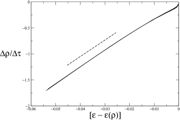
Figure 1: $\dot{\rho}\equiv\Delta\rho/\Delta\tau$ versus $\epsilon-\epsilon(\rho)$ for $\alpha=2.5$ and $v=2.4,\,2.45,\,2.5,\,2.53$. The dashed line is the best–fit of the slope ($-\gamma\approx 30$), common to all values of $v$ . It has been drawn to guide the eyes for appreciating the extension of the transient evolution, during which the four lines overlap.

For larger values of time, $\rho(t)$ decreases linearly in time, as predicted by Eq.(6.88). This confirms the presence of the phenomenon of gelation, according to which the system reaches a denutared state in a finite time (see Fig.2).

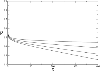
Figure 2: The density of H-bonds $\rho$ as a function of $\tau$ for $\alpha=2.5$ and $v=2.4,\,2.45,\,2.5,\,2.53$ (from top to bottom). Note that a linear decrease in time is eventually approached, thus yielding denaturation after a finite time (gelation phenomenon).

We have not been able to check the quantitative agreement with the theoretical predictions reported in subsection A. In particular, we have not found an effective criterion for locating the crossover between the initial and the asymptotic dynamics of $\rho(t)$. It is expected to occur at the critical time $t_{c}$ ($\rho(t_{c})=\rho_{c}$), but in MC simulations the crossover region extends over a long time lapse, which typically begins before and extends far beyond $t_{c}$. We want to point out that such a scenario is not unexpected: finite-size and memory effects cannot allow for the identification of a single transition point between the two dynamical regimes. This analysis could be slightly improved by considering much larger lattices and longer simulations, while maintaining at least the same number of averages over initial conditions. We did not proceed along this line, because the limit of our computational capabilities has already been reached with the values adopted in the reported simulations.

This scenario does not change also for $v<v_{c}$ ($T<T_{c}$) . We still find a qualitative agreement with the theoretical predictions based on the order parameter dynamics. Specifically, for small times the dynamics is again ruled by $\dot{\rho}=-\gamma[\epsilon_{\rho}-\epsilon]$ (see Fig.3) .

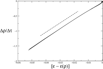
Figure 3: $\dot{\rho}\equiv\Delta\rho/\Delta\tau$ versus $\epsilon-\epsilon(\rho)$ for $\alpha=2.5$ and $v=2.2,\,2.25,\,2.3,\,2.33$. The dashed line is the best–fit of the slope ($-\gamma\approx 30$), common to all values of $v$ . It has been drawn to guide the eyes for appreciating the extension of the transient evolution, during which the four lines overlap.

Afterwards, one observes the decay to a finite asymptotic value $\rho_{\epsilon}>\rho_{c}$ (see Fig.4) . According to Eq.(6.89) such a decay is predicted to be exponential, with the decay rate $\tau$ given in Eq.(6.90) .

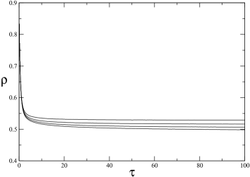
Figure 4: The density of H-bonds $\rho$ as a function of $\tau$ for $\alpha=2.5$ and $v=2.2,\,2.25,\,2.3,\,2.33$ (from top to bottom). Note that the decay to a finite value $\rho_{\epsilon}$ slows down significantly as $v$ approaches $v_{c}=2.34\pm 0.02$.

Also in this case a clear quantitative verification is prevented by the long lapse of time characterizing the crossover between the transient and the asymptotic dynamics.

Further peculiar behaviors of the microscopic dynamics emerge for $v>v_{c}$ and $\rho(0)<\rho_{c}$. In this case any initial condition cannot correspond to an equilibrium state. Accordingly, hysteretic effects determine a growth of $\rho(t)$ from $\rho(0)$, until a value close to $\rho_{c}$ is approached. Then, $\rho(t)$ starts to decrease until a linear–in–time decay is eventually approached, as predicted by Eq.(6.87) (as an example, see Fig.5) .

Figure 5: The density of H-bonds $\rho$ as a function of $\tau$ for $\alpha=2.5$ and $v=2.6$. The evolution has been obtained by averaging over randomly seeded initial conditions of initial density $\rho(0)=0.8$ and 0.4 . In order to better appreciate the hysteretic effect associated with the first–order nature of the phase transition (lower curve), we have reported the evolution over a relatively short time scale. Note also that the initial conditions affect only the transient evolution: both curves converge to the same asymptotic dynamics, which eventually turns out to a linear–in-time decay, yielding the gelation phenomenon.

The phenomenon of gelation is recovered also in this case, as predicted on the basis of the order parameter equation. Nonetheless, a quantitative analysis is prevented for the above mentioned reasons.

2. The case $\alpha=1.5$

Numerical analysis predicts a critical value of the control parameter $v_{c}=3.60\pm 0.02$. This result agrees quite well with the theoretical expectation $v_{c}=3.6060508...$. On the other hand, the crossover between the transient and the asymptotic dynamics is found to extend much more than in the case $\alpha=2.5$. For instance, even very close to $v_{c}$ the transient behavior ruled by the law $\dot{\rho}=-\gamma[\epsilon_{\rho}-\epsilon]$ lasts over a few units of $\tau$ (see Fig.6). Such a linear region reduces the more $v$ is far from $v_{c}$

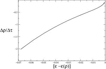
Figure 6: $\dot{\rho}\equiv\Delta\rho/\Delta\tau$ versus $\epsilon-\epsilon(\rho)$ for $\alpha=1.5$ and $v=3.59,\,3.60,\,3.61$. A linear dependence can be attributed to the first few units of $\tau$.

However, the long–time dynamics allows to identify the occurrence of the gelation phenomenon for $v>v_{c}$ ($T>T_{c}$). In particular, $\rho$ eventually exhibits a decay in time which is faster than linear. In order to exemplify this behavior in Fig.7 we show $\rho(\tau)$ for some values of $v$ much larger than $v_{c}$. The asymptotic behavior is ruled by a decay faster than a power-law, but also slower than an exponential. This finding confirms the qualitative agreement with the predicitons of the order parameter dynamics.

Figure 7: The density of H-bonds $\rho$ as a function of $\tau$ for $\alpha=1.5$ and $v=3.8,\,4.5,\,6.0$ (from top to bottom) . The double–logarithmic scale shows an aymptotic decay in time which is faster than linear.

We want to point out that we have reported the results for large values for $v$, because this choice allows to reduce the duration of the crossover from the transient regime. In fact, for the same values of $v$ reported in Fig.6 the long–time behavior sets in for much larger values of $\tau$. Moreover, note that also in these cases finite size effects do not allow to reach a completely denaturated state ($\rho=0$). In fact the long time dynamics exhibits fluctuations around a low-density regime which is not shown in Fig.7.

Also for $v<v_{c}$ (i.e. $T<T_{c}$) the transient dynamics $\dot{\rho}=-\gamma[\epsilon_{\rho}-\epsilon]$ lasts for very short times and crosses over to a slow relaxation to the asymptotic non-zero equilibrium value of the density, $\rho_{\epsilon}$. As for the case $\alpha=2.5$, a quantitative study concerning the scaling analysis associated with the exponential decay rate cannot be worked out satisfactorily with our computational resources.

Despite all the difficulties inherent MC simulations, we can conclude that it exhibits a remarkable qualitative agreement with the order parameter dynamics discussed in this Section.

VII Summary

In this paper we have derived new results for the classical Lifson-Poland-Sheraga model of DNA denaturation. In the first part we have reviewed the main equilibrium properties and completed the list of known results by the computation of one- and two-point correlation functions and structure factors, including scaling formulas for the latter. In the second part we have investigated the dynamical properties of this model, both numerically and analytically. The Langevin equation written for the density of H-bonds has been solved with and without the noise term, in the second case in a linear approximation. Scaling laws for different values of $\alpha$ have been obtained, and a gelation phenomenon — arrival to equilibrium in a finite time — above the critical temperature has been identified. Remarkably, in the cases when comparison was possible, we have found that the predictions of the phenomenological theory were practically indistinguishable from the numerical findings.

Our results suggest that the LPS model belongs to a new universality class, in the language of critical phenomena, so that most of its details do not matter near the critical point. This is confirmed by both the static structure factor and the dynamics of the order parameter. Concerning the dynamics, the surprising success of the equation of the order parameter compared with the more detailed description by the master equation has its counterpart in usual treatments of critical phenomena. A theoretical explanation of this universality might be given by a renormalization group analysis of models of the helix-coil transition that are more microscopic than the LPS one. However, the best test of universality would be experimental. We hope that our work will stimulate such experiments, so that the very nature of the DNA denaturation transition could finally be clarified. A better understanding of the gelation phenomenon characterizing the high-temperature phase is also missing. Is this phenomenon basically related to the long–range nature of the effective interaction of the LPS model? To our knowledge no systematic investigation has been performed for identifying such a phenomenon in biomolecules.

Note added: After finishing the analytic part of our work two papers BKM , SK have appeared on the preprint archive, dealing with the dynamics of the helix-coil transition. Our approach is, however, sensibly different.

Acknowledgments — We would like to express our gratitude to the Departments of Physics of the Ecole Polytechnique Fédérale de Lausanne and the University of Florence, where the major part of this work was done. We specially thank Prof. Harald Posch for his kind hospitality at the Institute of Experimental Physics of the University of Vienna, where our paper was completed. The work of A.S. was supported by OTKA Grants T 043494 and T 046129. R.L. wants to thank the Italian Ministry of University and Research (MIUR), which supported his work through the FIRB project RBAU01BZJX .

References

- (1) S. Lifson, J. Chem. Phys. 40, 3705 (1964)
- (2) D. Poland and H.A. Sheraga,J. Chem. Phys. 45, 1456 (1966)
- (3) M.S. Causo, B. Coluzzi, P. Grassberger, Phys. Rev. E 62, 3958 (2000).
- (4) E. Carlon, E. Orlandini and A.L. Stella, Phys. Rev. Lett. 88, 198101 (2002).
- (5) M.Baiesi, E. Carlon and A.L. Stella, Phys. Rev. E 66, 021804 (2002).
- (6) M.Baiesi, E. Carlon, Y. Kafri, D. Mukamel, E. Orlandini and A.L. Stella, Phys. Rev. E 67, 021911 (2003).
- (7) L. Schäfer, cond-mat 0502668 (2005)
- (8) Y. Kafri, D. Mukamel and L. Peliti, Phys. Rev. Lett. 85, 4988 (2000)
- (9) R. Blossey and E. Carlon, Phys. Rev. E 68, 061911 (2003).
- (10) R.M. Wartell and A.S. Benight, Phys. Rep. 126, 67 (1985).
- (11) R.D. Blake and S.G. Delcourt, Nucleic Acids Res. 26, 3323 (1998).
- (12) G: Zocchi et al., cond-mat 0304567 (2003).
- (13) M. Peyrard and A.R. Bishop, Phys. Rev. Lett. 62, 2755 (1989).
- (14) N. Theodorakopoulos, T. Dauxois and M. Peyrard, Phys. Rev. Lett. 85, 6 (2000).
- (15) D.R. Nelson, cond-mat 0309559 (2003).
- (16) R.M. Ziff, E.M. Hendriks and M.H. Ernst, Phys. Rev. Lett. 49, 593 (1982).
- (17) A. Bar, Y. Kafri and D. Mukamel, cond-mat/0608663
- (18) A. Santos and W. Klein, cond-mat/0610484