Dissipation: The phase-space perspective

Abstract

We show, through a refinement of the work theorem, that the average dissipation, upon perturbing a Hamiltonian system arbitrarily far out of equilibrium in a transition between two canonical equilibrium states, is exactly given by $\langle W_{diss}\rangle=\langle W\rangle-\Delta F=kTD(\rho\|\widetilde{\rho})=kT\langle\ln(\rho/\widetilde{\rho})\rangle$, where $\rho$ and $\widetilde{\rho}$ are the phase space density of the system measured at the same intermediate but otherwise arbitrary point in time, for the forward and backward process. $D(\rho\|\widetilde{\rho})$ is the relative entropy of $\rho$ versus $\widetilde{\rho}$. This result also implies general inequalities, which are significantly more accurate than the second law and include, as a special case, the celebrated Landauer principle on the dissipation involved in irreversible computations.

Since the pioneering work of Boltzmann, the search for an exact microscopic expression of dissipation has been at the heart of (nonequilibrium) statistical mechanics. In this letter, we derive such an expression from first principles, through a refinement of the recently discovered work theorem by Jarzynski and Crooks jarzynski .

The second law of thermodynamics stipulates that the average mechanical work $\langle W\rangle$ needed to move a system in contact with a heat bath at temperature $T$, from one equilibrium state $A$ into another equilibrium state $B$, is at least equal to the free energy difference between these states: $\langle W\rangle\geq\Delta F=F_{B}-F_{A}$. The equality is reached for a quasi-static process. The extra work $\langle W\rangle-\Delta F$ is often referred to as the dissipated work. Contrary to the reversible work, the dissipated work depends on how the transition between the states is realized. Typically, one or more external control parameters are changed in time, following a specific protocol, between initial an final values. The dissipated work will depend on this protocol, which can in principle bring the system arbitrarily far out of equilibrium. Amazingly, there exists an exact, simple and compact microscopic expression for this dissipation. The key is to consider the protocol and its time-reversed version. We will refer with a superscript tilde to all the quantities measured in the time-reversed protocol. The central result is then the following: $\langle W_{diss}\rangle=\langle W\rangle-\Delta F=kTD(\rho||\tilde{\rho})=kT\langle\ln(\rho/\widetilde{\rho})\rangle$, where $\rho$ and $\widetilde{\rho}$ are the phase space densities of the system measured at the same intermediate but otherwise arbitrary point in time, in the forward and backward protocol, respectively. $D(\rho\|\widetilde{\rho})$ is the Kullback-Leibler distance cover , also called relative entropy, of $\rho$ versus $\widetilde{\rho}$.

The derivation is similar in spirit to that of the Jarzynski and Crooks equalities jarzynski . Consider a Hamiltonian $H(q,p;\lambda)$ where $(q,p)$ represents the set of position and momentum variables of the system under consideration and $\lambda$ is a control parameter which is varied from an initial value $\lambda_{A}$ to a final value $\lambda_{B}$ according to a protocol $\lambda(t)$ controlled by an external agent. The system is initially assumed to be in canonical equilibrium at temperature $T$ at the value $\lambda_{A}$ of the control parameter and, along the protocol, is completely isolated, i.e., no energy is exchanged other than the work $W$ performed by the external agent on the system. In the time-reversed scenario, the system is initially at canonical equilibrium at the same temperature $T$, but at the value $\lambda_{B}$ of the control parameter, which is now changed according to the exact time-reversed protocol.

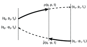
Figure 1: Space-time coordinates for the forward and backward trajectories.

We first set out to calculate the work $W(q,p\,;t)$ done along the whole process, for the specific phase trajectory that passes through the phase point $(q,p)$ at time $t$. Since the dynamics are deterministic, there is precisely one such trajectory. Let us call $(q_{0},p_{0})$ and $(q_{1},p_{1})$ the corresponding initial and final phase points. Note also that there is a one-to-one correspondence with the time-reversed trajectory in the time-reversed protocol which, starting from $(q_{1},-p_{1})$, goes through $(q,-p)$ and finally into $(q_{0},-p_{0})$, cf. Fig. 1. For simplicity of notation, we will use the forward time to express times in both forward and backward scenarios. By conservation of total energy, one has that:

$$W(q,p;t)=H(q_{1},p_{1};\lambda_{B})-H(q_{0},p_{0};\lambda_{A})\\$$ (1)

Now, since the phase space density is conserved along any Hamiltonian trajectory, one has, in both forward and backward process:

$$\rho(q,p,t)=\rho(q_{0},p_{0},t_{0}) = \frac{\exp[-\beta H(q_{0},p_{0};\lambda_{A})]}{Z_{A}}$$ (2)

$$\widetilde{\rho}(q,-p,t)=\widetilde{\rho}(q_{1},-p_{1},{t}_{1}) = \frac{\exp[-\beta H(q_{1},-p_{1};\lambda_{B})]}{Z_{B}}$$

where $Z_{A}$ and $Z_{B}$ are partition functions at the equilibrium states $A$ and $B$, respectively. These expressions allow us to eliminate the Hamiltonian (which is supposed to be even in the momenta, or more precisely time-reversible) at initial and final times in favor of the phase space density at any intermediate time point. Eq. (1), yields the following generalized Crooks relation:

$$\exp\left\{\beta[W(q,p;t)-\Delta F]\right\}=\frac{\rho(q,p,t)}{\widetilde{\rho}(q,-p,t)}$$ (3)

where $\Delta F=-kT(\ln Z_{B}-\ln Z_{A})$ is the free energy difference between the final and initial equilibrium states. If we now rewrite Eq. (3) as follows:

$$W(q,p;t)-\Delta F=kT\ln\frac{\rho(q,p,t)}{\widetilde{\rho}(q,-p,t)}\;,$$ (4)

the average work reads:

$$\langle W\rangle-\Delta F = kT\int dqdp\,\,\rho(q,p,t)\ln\frac{\rho(q,p,t)}{\widetilde{\rho}(q,-p,t)}$$ (5)

$$= kTD\big{(}\rho(q,p,t)\|\widetilde{\rho}(q,-p,t)\big{)}.$$

We conclude that the dissipated work is fully revealed by the phase space density of forward and backward processes at any intermediate time of the experiment. It is particularly interesting to note that this dissipation, cf. r.h.s. of Eq. (5), takes the form of the relative entropy (Kullback-Leibler distance cover ) $D(\rho\|\widetilde{\rho})=\int dqdp\,\,\rho\ln(\rho/\widetilde{\rho})$ between the forward and backward probability distributions $\rho$ and $\tilde{\rho}$. This simple result calls for a number of more specific comments. First, since a relative entropy is strictly non-negative, we conclude that the dissipation cannot be negative, in agreement with the second law. Second, the dissipation results from the asymmetry between the forward and backward protocols: it is zero only when $\rho(q,p,t)=\widetilde{\rho}(q,-p,t)$. In fact, Stein’s lemma cover relates $D(\rho\|\widetilde{\rho})$ directly to the difficulty of statistically distinguishing forward versus backward trajectories. This is consistent with the general observation that dissipation is the result of the breaking of detailed balance maes . The above expression is also consistent with a proposal, linking the time-asymmetry of the Kolmogorov-Sinai entropy to the entropy production of the dynamical system gaspard . Third, the total dissipation, cf. the l.h.s. of Eq. (5), is obviously a constant, independent of time. Yet the densities in the r.h.s. of Eq. (5) can be evaluated at any intermediate time $t$. This time-independence follows from the observation that the relative entropy of densities obeying the same Liouville equation, is constant in time mackey . Fourth, the evaluation of the dissipated work in general requires full knowledge of the phase space density, even though only at one particular instant of time. That such detailed information may be needed is consistent with the generality of the result, which is valid no matter how far the system is driven out of equilibrium. However, one can get away from this apparently stringent requirement, by invoking the chain rule for relative entropy cover . According to this rule, the relative entropy decreases upon coarse graining. The equality Eq. (5) is then replaced by an inequality. It is instructive to give a direct derivation of this result.

Consider a partition of the entire phase space, consisting of $K$ non-overlapping subsets $\chi_{j},\,(j=1,\dots,K)$. We introduce the corresponding coarse grained phase densities

$$\rho_{j}=\int_{\chi_{j}}\rho(q,p)dqdp\,;\quad\widetilde{\rho}_{j}=\int_{\widetilde{\chi}_{j}}\widetilde{\rho}(q,-p,t)dqdp$$

where the $\widetilde{\chi}_{j}$ is identical to $\chi_{j}$, apart from the inversion of all momenta. By integration of Eq. (3) over the set $\chi_{j}$, we obtain the following detailed Jarzynski equality:

$$\langle e^{-\beta W}\rangle_{j}=\frac{\int_{\chi_{j}}\rho(q,p,t)e^{-\beta W(q,p;t)}dqdp}{\rho_{j}}=\frac{\widetilde{\rho}_{j}}{\rho_{j}}e^{-\beta\Delta F}$$ (6)

By Jensen’s inequality, Eq. (6) implies a second-law like inequality:

$$\langle W\rangle_{j}\geq\Delta F+kT\ln\left(\frac{\rho_{j}}{\widetilde{\rho}_{j}}\right)\geq-\langle\widetilde{W}\rangle_{j}\,.$$ (7)

where we have included, for later reference, the inequality that arises by considering the backward process. Finally, by performing an average over the different subsets, one finds:

$$\langle W\rangle = \sum_{j}\rho_{j}\langle W\rangle_{j}\geq\Delta F+kTD(\rho_{j}\|\widetilde{\rho}_{j})$$ (8a)

$${\langle\widetilde{W}\rangle} = \sum_{j}\widetilde{\rho}_{j}\langle\widetilde{W}\rangle_{j}\geq-\Delta F+kTD(\widetilde{\rho}_{j}\|\rho_{j})\,.$$ (8b)

where the discrete version of relative entropy is defined by $D(\rho_{j}\|\widetilde{\rho}_{j})=\sum_{j}\rho_{j}\ln(\rho_{j}/\widetilde{\rho}_{j})$.

We conclude that, when full information of the phase density is not available, a coarse grained relative entropy still provides a lower bound for the dissipative work, significantly improving the classical one given by the second law. How well this bound approaches the total dissipation will depend on how far the process is from the quasi-static regime. In particular, in the latter case, any partition will do, and the relative entropy is always identically zero. More interestingly, one expects that a coarse-grained partition will suffice in case of separation of time scale between fast and slow variables. Indeed, in this case and for a protocol on the slow time scale, the fast variables will be essentially at equilibrium and all the dissipation is captured in the time-asymmetry contained in the slow variables. We note however that in this reduced set of variables, trajectories can, unlike in full phase space, cross each other. A more detailed analysis reveals that full information is then not captured by measurement at a single time, but should in general be carried out at all times, in agreement with, e.g., the entropy production of Markovian processes maes ; gaspard ; lebowitz .

To illustrate the power and usefulness of our results, we turn to a number of specific examples. We first consider the quenching of a system described by the Hamiltonian $H(x;\lambda)$, in contact with a heat bath at temperature $T$. The equilibrium probability distribution to observe the state $x$ is given by a Boltzmann distribution $p(x;\lambda)\equiv\exp(-\beta H(x;\lambda))/Z_{\lambda}$ with $Z_{\lambda}$ the normalization factor (partition function). We now perturb this equilibrium by the following irreversible quench: the control parameter is changed instantaneously from the value $\lambda$ to the value $\lambda^{\prime}$ at a specific time and the experiment terminates at any later time. In the backward process, we start from equilibrium at $\lambda^{\prime}$ and quench back to $\lambda$. Since the state $x$ does not change during the instantaneous quench, the work in the forward process is:

$$\langle W\rangle=\int\textrm{d}x\;\;[H(x;\lambda^{\prime})-H(x;\lambda)]\;\;p(x;\lambda)$$ (9)

Now consider a partition, infinitely fine in the position coordinates (disregarding all the other degrees of freedom, in particular those of the heat bath) and measure the coarse grained distribution $p(x,t)$ at the time of quench. We note that the distributions prior to the quench are the equilibrium distribution from which one started, i.e., $p(x;\lambda)$ and $p(x;\lambda^{\prime})$ for forward and backward scenario respectively. Turning to Eq. (7), the role of $\rho_{j}$ and $\widetilde{\rho}_{j}$ are thus played by $p(x;\lambda)$ and $p(x;\lambda^{\prime})$, hence:

$$\langle W\rangle\geq\Delta F+kT\int\textrm{d}x\;\;p(x;\lambda)\;\;\ln\frac{p(x;\lambda)}{p(x;\lambda^{\prime})}$$ (10)

Using the Boltzmann probability distributions together with $\Delta F=-kT\ln(Z_{\lambda^{\prime}}/Z_{\lambda})$, a comparison with Eq. (9) reveals that the equality sign holds in Eq. (10). We conclude that in this case the coarse-grained partition captures the full dissipation.

Turning to a more complicated situation, we consider an overdamped Brownian particle in contact with a heat bath at temperature $T$, moving in a harmonic potential whose spring constant varies from $\kappa$ to $\kappa^{\prime}$ during a finite time $\tau$. For $\tau\rightarrow 0$, one recovers the quenching experiment described above with $\langle W\rangle$ given by Eq. (9) (with a harmonic Hamiltonian). For $\tau\rightarrow\infty$, one approaches the quasi-static limit with $\langle W\rangle=\Delta F$. In Fig. 2 we compare the dissipative work $\langle W\rangle-\Delta F$, obtained from Langevin simulations, with the relative entropy measured at the middle of the transition with a fine partition ($\Delta x=0.1$) and a coarse partition ($\Delta x=1.0$). The relative entropy is always below the dissipative work, consistent with Eq. (8a). For the fine partition the relative entropy coincides with the dissipative work as $\tau$ approaches the quenched limit, in agreement with Eq. (10). Note that the refinement of the partition in estimating the dissipation is most effective close to the quenched limit.

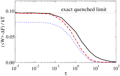
Figure 2: Dissipation of Brownian particles in a harmonic potential with spring constant varying from $\kappa=2$ to $\kappa^{\prime}=1$ during a time interval $\tau$. Solid line is dissipative work directly obtained from simulation. Dashed and dotted lines indicate the lower bound of the dissipative work estimated from the relative entropy.

In our final illustration, we show that Eqs. (8) include as a special case the celebrated Landauer principle on the minimal dissipation of irreversible computations. We consider a Brownian computer landauer ; bennett ; others , consisting of a one-dimensional overdamped Brownian particle at temperature $T$ in a time-dependent potential varied by an external agent according to a given cyclic protocol shown in Fig. 3. Since it involves spontaneous symmetry breaking followed by forced symmetry breaking, this process is analogous to the Szilard engine parrondo , whereas the reverse, starting from b, is analogous to the Landauer’s restore-to-zero process leff ; landauer ; bennett .

The coarse resolution measurement is made at the stage b of the forward cycle by partitioning position space into two sets, $\chi_{R}=\{x:x\geq 0\}$ and $\chi_{L}=\{x:x<0\}$ (See Fig. 3). In the forward process, we have by symmetry that $p_{R}=p_{L}=1/2$. In the backward process the large majority of trajectories will be forced by the external bias towards the location of the cell $\chi_{R}$ at stage d. However, since the height of the barrier is finite, trajectories can still thermally cross over to $\chi_{L}$ before reaching the filtering stage b. Therefore, the probabilities $\widetilde{p}_{R}$ and $\widetilde{p}_{L}$, while being close to $1$ and $0$ for strong forcing, will otherwise depend on the applied force, barrier height, temperature and processing speed.

In this example, we focus on the validity of Eq. (7), i.e., the average work for each macroscopic trajectory, $R$ or $L$. For strong forcing, $\widetilde{p}_{R}=1$, Eq. (7) reads:

$$\langle W\rangle_{R}\geq-kT\ln 2\geq-\langle\widetilde{W}\rangle_{R}\;\;\;\;(\widetilde{p}_{R}=1).$$ (11)

This expression includes Landauer’s principle in the case of the backward process, namely, that the erasure of one bit of information must be accompanied by the dissipation of an energy $kT\ln 2$. For the Szilard engine, i.e., the forward process, one recovers the apparent violation of the second law by $R$ trajectories when the equal sign in Eq. (11) holds: $\langle W\rangle_{R}=-kT\ln 2$. Concomitantly, along the $L$ path, we have $\tilde{p}_{L}\rightarrow 0$, or, more precisely, $\tilde{p}_{L}\approx\exp(-V/kT)$, $V$ being the height of the barrier, and the lower bound given by Eq. (8a) is, approximately, $\langle{W}\rangle_{L}>V$. The $L$ trajectories correspond to a “wrong” measurement in the Szilard engine parrondo , and they dissipate an energy significantly bigger than the energy $kT\ln 2$ extracted from the thermal bath in the $R$ trajectories. Consequently, the overall dissipation for the engine is positive, in accordance with the second law.

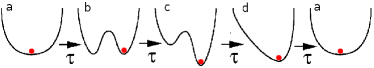
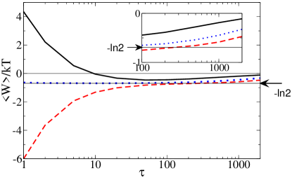
Figure 3: Top: Cyclic variation of a model potential. The arrows indicate the forward protocol corresponding to the Szilard engine. The backward process is a model for recording and erasing information. Bottom: Partitioned average work as a function of processing time $\tau$: $\langle W\rangle_{R}$ (solid line) and $-\langle\widetilde{W}\rangle_{R}$ (dashed line). The bound (7) using the coarse grained distribution is shown by the dotted line.

In Fig. 3 we show the results of numerical simulations of the corresponding overdamped Langevin equation. Average work performed by the Brownian particles residing in the right well at the stage b in the forward and backward processes is plotted for different values of the processing time $\tau$. The bound using $p_{R}$ and $\widetilde{p}_{R}$ measured directly in the simulation is also plotted. The bound is always between $\langle W\rangle_{R}$ and $-\langle\widetilde{W}\rangle_{R}$ in agreement with Eq. (7). Note that the Landauer principle, contained in (11), breaks down in the quasi-static limit $\tau\rightarrow\infty$, since the Brownian particle equilibrates by crossing the barrier. In this process, the stored information is lost, $\widetilde{p}_{R}\rightarrow 1/2$, and the (dissipated) work goes to zero. Nevertheless, the inequality (7) is always satisfied.

As the Jarzynksi equality itself has generated a lot of debate, a critical discussion of the above theory is in place. The term dissipation is usually associated to entropy production. To make this connection, we note that the system is not at equilibrium at the final stage of the (forward) experiment. We can however reconnect it to a heat reservoir and let it relax to its canonical equilibrium state for $\lambda=\lambda_{B}$ and temperature $T$. In doing so, it will exchange the dissipated work under the form of heat with the bath, resulting in an entropy production $\Delta S=k\langle\ln(\rho/\widetilde{\rho})\rangle$. One could ask whether the disconnection or reconnection of the system with the bath adds significant terms to the work and/or the free energy. Apart from the answers given to these issues in the context of the Jarzynski equality itself jarzynksireply , we are concerned here with the average total work, which is much larger than these energies for large systems and long enough operation times. Finally, the above derivation relies on a continuous transformation of the Hamiltonian, excluding, for example, free expansion. This limitation reflects the need for considering the time-reversed process.

This collaboration was supported by the StochDyn program of the European Science Foundation. J.M.R.P. acknowledges financial support from Ministerio de Educación y Ciencia (Spain), grant FIS04-271, and from BCSH, grant UCM PR27/05-13923- BSCH.

References

- (1) C. Jarzynski, Phys. Rev. Lett., 78, 2690 (1997); G. E. Crooks, J. Stat. Phys. 90, 1481 (1998).
- (2) T. M. Cover and J. A. Thomas, Elements of Information Theory, (Wiley, Hoboken, New Jersey, 2nd ed., 2006).
- (3) C. Maes, Poincare Seminar, pp. 145, edited by Dalibard B.D.J. and Rivasseau V. Birkhauser, Basel (2003).
- (4) P. Gaspard, J. Stat. Phys. 117, 599 (2004).
- (5) M. C. Mackey, Rev. Mod. Phys. 61, 981 (1989).
- (6) J. L. Lebowitz and H. Spohn, J. Stat. Phys. 95, 333 (1999).
- (7) L. Szilard, Z. Physik 53, 840 (1929).
- (8) H. S. Leff. and A. F. Rex, Maxwell’s Demon 2, (Institute of Physics Philadelphia, 2nd ed., 2003).
- (9) R. Landauer, IBM J. Res. Dev. 5, 183, (1961).
- (10) C. H. Bennett, Int. J. Theor. Phys. 21, 905 (1982); B. Piechocinska, Phys. Rev. 61, 062314 (2000).
- (11) K. Shizume, Phys. Rev. E 52, 3495 (1995); K. Sekimoto, Stochastic Energetics, (Iwanami, Tokyo, 2005).
- (12) J. M. R. Parrondo, Chaos 11, 725 (2001).
- (13) C. Jarzynski, J. Stat. Mech.: Theor. Exp. P09005 (2004).