Valence-band mixing in first-principles envelope-function theory

Abstract

This paper presents a numerical implementation of a first-principles envelope-function theory derived recently by the author [B. A. Foreman, Phys. Rev. B 72, 165345 (2005)]. The examples studied deal with the valence subband structure of GaAs/AlAs, GaAs/Al_0.2Ga_0.8As, and In_0.53Ga_0.47As/InP (001) superlattices calculated using the local density approximation to density-functional theory and norm-conserving pseudopotentials without spin-orbit coupling. The heterostructure Hamiltonian is approximated using quadratic response theory, with the heterostructure treated as a perturbation of a bulk reference crystal. The valence subband structure is reproduced accurately over a wide energy range by a multiband envelope-function Hamiltonian with linear renormalization of the momentum and mass parameters. Good results are also obtained over a more limited energy range from a single-band model with quadratic renormalization. The effective kinetic-energy operator ordering derived here is more complicated than in many previous studies, consisting in general of a linear combination of all possible operator orderings. In some cases the valence-band Rashba coupling differs significantly from the bulk magnetic Luttinger parameter. The splitting of the quasidegenerate ground state of no-common-atom superlattices has non-negligible contributions from both short-range interface mixing and long-range dipole terms in the quadratic density response.

I Introduction

In a recent paper, the author has developed a first-principles multiband envelope-function theory for semiconductor heterostructures. Foreman (2005) This theory can in principle provide accurate numerical predictions of envelope-function Hamiltonian parameters, but only if a reliable quasiparticle self-energy is used as input. On the other hand, if the input potential is taken from a simple density-functional calculation, Foreman (2007a) the numerical values are less accurate, but the theory can still provide deep insight into the basic physics of the interface and clarify various limitations of commonly used envelope-function models. The purpose of the present article is to explore these topics using numerical examples taken from density-functional calculations of the valence subband structure in semiconductor superlattices.

In order to obtain the most direct comparison with envelope-function theory as it is commonly used, the Hamiltonian was derived in Ref. Foreman, 2005 in the form of a matrix containing differential operators and energy-independent functions of position. Using a differential equation of low order to describe an abrupt heterojunction might seem at first glance to be a gross theoretical blunder, since it is well known that bulk effective-mass theory Luttinger and Kohn (1955) is valid only for slowly varying perturbing potentials. Yet effective-mass theory is widely accepted as a valid lowest-order approximation for the shallow impurity problem, Kohn (1957); Bassani et al. (1974); Pantelides (1978) even though the atomic impurity potential is not slowly varying. Its validity in this context is established by the existence of rigorous methods for extending effective-mass theory to include higher-order perturbations, Bassani et al. (1974); Pantelides (1978); Sham (1966) including the rapidly varying part of the impurity potential. Bir and Pikus (1974) These produce short-range and long-range corrections to the effective Hamiltonian (each with its own independent parameters), which lead to the well known chemical shift and splitting of effective-mass degeneracies, Bassani et al. (1974); Pantelides (1978); Bir and Pikus (1974) thereby bringing the rough estimates of effective-mass theory into much closer agreement with experiment.

A heterostructure is nothing but an assembly of atoms. It is therefore difficult to imagine a valid argument for accepting the use of generalized effective-mass differential equations in the shallow impurity problem, yet categorically rejecting them for small atomic perturbations in heterostructures. According to linear response theory, the perturbation generated by a collection of small atomic perturbations is to leading order just the superposition of the individual perturbations. The rapidly varying part of the heterostructure potential Burt (1992); Takhtamirov and Volkov (1999) can thus be handled by the same techniques used in the impurity problem. Bir and Pikus (1974) The validity of low-order differential equations for shallow heterostructures—as for shallow impurities—consequently rests on two fundamental assumptions: Luttinger and Kohn (1955); Bir and Pikus (1974) that the envelope functions satisfying these equations are slowly varying Burt (1992) (i.e., have a Fourier transform limited to small wave vectors) within the energy range of experimental interest, and that the atomic perturbations are truly “shallow” in real heterostructures.

The first assumption is confirmed by numerical examples in later sections of this paper, in agreement with prior empirical pseudopotential studies. Xia (1989); Wang et al. (1997); Wang and Zunger (1997, 1999) For the second assumption, the definition of “shallow” is a relative one that depends on the energy separation between the states included explicitly in the envelope-function model and the remote states treated as perturbations [see, e.g., Eq. (II.33) of Ref. Luttinger and Kohn, 1955]. Consider the case of a GaAs/AlAs heterostructure, where the valence-band offset is about 0.5 eV and the energy gap is about 1.5 eV. Treating GaAs/AlAs as a shallow perturbation of the virtual crystal Al_0.5Ga_0.5As would be expected to yield marginal results (at best) in a single-band effective-mass model for the degenerate $\Gamma$ valence states. Such a model would be expected to give good results only for weaker perturbations, such as those in a GaAs/Al_0.2Ga_0.8As heterostructure (within the virtual-crystal approximation). On the other hand, treating GaAs/AlAs as a shallow perturbation would be expected to produce good results in a multiband envelope-function model that includes a few of the nearest conduction-band states explicitly, since the remote bands are then more than 5 eV away from the valence-band maximum. (This method of making moderately “deep” perturbations “shallow” by including more bands in the Hamiltonian was proposed by Keldysh for the deep impurity problem in bulk semiconductors.Keldysh (1964)) All of the above expectations are confirmed below by numerical examples for GaAs/Al_0.2Ga_0.8As, GaAs/AlAs, and In_0.53Ga_0.47As/InP.

To be more specific, the multiband envelope-function Hamiltonian of Ref. Foreman, 2005 was derived by treating the heterostructure as a perturbation (within the pseudopotential approximation) of a virtual bulk reference crystal. The self-consistent potential energy of the heterostructure was approximated using the linear and quadratic terms of nonlinear response theory (see the preceding paper Foreman (2007a) for further details). A finite-order envelope-function Hamiltonian was constructed by using Luttinger–Kohn perturbation theory Luttinger and Kohn (1955); Bir and Pikus (1974); Leibler (1975, 1977) to eliminate the $\mathbf{k}\cdot\mathbf{p}$ and potential-energy coupling to remote bands, working to order $k^{4}$ in the bulk reference Hamiltonian, Takhtamirov and Volkov (1999) to order $k^{2}$ in the linear response terms, Leibler (1975, 1977) and to order $k^{0}$ in the quadratic response. Takhtamirov and Volkov (1999) This theory is shown here to work well in a 3-state model for the $\Gamma_{15\mathrm{v}}$ valence states (i.e., neglecting spin-orbit coupling) of a GaAs/Al_0.2Ga_0.8As superlattice and in a 7-state $\{\Gamma_{15\mathrm{c}},\Gamma_{1\mathrm{c}},\Gamma_{15\mathrm{v}}\}$ model for GaAs/AlAs and In_0.53Ga_0.47As/InP superlattices. Examples illustrating the success of a 4-state $\{\Gamma_{1\mathrm{c}},\Gamma_{15\mathrm{v}}\}$ model for In_0.53Ga_0.47As/InP superlattices have been given elsewhere. Foreman (2007b)

To test the limits of the single-band ($\Gamma_{15\mathrm{v}}$) model, this paper also extends the theory of Ref. Foreman, 2005 to include terms of order $\theta^{2}k$ and $\theta^{2}k^{2}$, where $\theta$ denotes the heterostructure perturbation. This is shown to yield much better predictions of the position-dependent effective masses of both GaAs/AlAs and In_0.53Ga_0.47As/InP than the $O(\theta^{1}k^{2})$ theory of Ref. Foreman, 2005. The resulting superlattice band structures are also of reasonably good accuracy, but over a more limited energy range than the multiband models. The principal limitation of the single-band theory seems to be the presence of spurious solutions generated by $O(\theta^{0}k^{4})$ terms in the bulk reference Hamiltonian.

The extended $O(\theta^{2}k^{2})$ theory also yields some interesting conclusions regarding operator ordering in the effective kinetic-energy operator $T$ in effective-mass theory. Much previous work has examined various possible ways of choosing the exponents $\alpha$, $\beta$, and $\gamma$ in the von Roos parametrization von Roos (1983)

$$T_{\mathrm{vR}}=\tfrac{1}{4}(m^{\alpha}pm^{\beta}pm^{\gamma}+m^{\gamma}pm^{\beta}pm^{\alpha}),$$ (1)

where $p$ is the momentum operator (in one dimension), $m$ is the effective mass, and $\alpha+\beta+\gamma=-1$. Morrow and Brownstein Morrow and Brownstein (1984, 1985) have argued that only exponents satisfying $\alpha=\gamma$ are physically permissible in abrupt heterostructures, which would rule out seemingly reasonable possibilities such as Gora and Williams (1969) $T=\tfrac{1}{4}(m^{-1}p^{2}+p^{2}m^{-1})$.

The present theory is not consistent with any single operator ordering of this type. Instead, the terms of order $p^{2}$ derived here take the form of a linear combination of terms containing position-dependent functions having all possible operator orderings with respect to $p$. The apparent conflict between this result and the theory of Morrow and Brownstein Morrow and Brownstein (1984, 1985) is resolved by the fact that these are smooth functions of position with no discontinuity even at an abrupt junction.

The structure of the paper is as follows. The quadratic-response theory used in the preceding article Foreman (2007a) to simplify the self-consistent pseudopotential is briefly reviewed in Sec. II. Section III describes the construction of the envelope-function Hamiltonian, which is also studied from the perspective of the theory of invariants. In Sec. IV, the parameters of the Hamiltonian are calculated and discussed for the material systems GaAs/AlAs, GaAs/Al_0.2Ga_0.8As, and In_0.53Ga_0.47As/InP. The valence subband structures for (001) superlattices of these materials are calculated in Sec. V, which compares the predictions of various approximate envelope-function models with “exact” numerical calculations. Finally, the results of the paper are discussed and summarized in Sec. VI.

II Quadratic-response theory

The foundations for this work were laid in the preceding article, Foreman (2007a) in which methods are developed for approximating the self-consistent heterostructure pseudopotential using quadratic-response theory. This section presents a brief summary of the main ideas.

All of the numerical results in this paper are taken from self-consistent total-energy calculations Payne et al. (1992); Martin (2004) performed in a plane-wave basis using the abinit software Gonze et al. (2002, 2005); ABI with nonlocal norm-conserving pseudopotentials and the local-density approximation (LDA) to density-functional theory. Spin-orbit coupling is neglected. This model was chosen in order to permit direct comparisons of envelope-function calculations with “exact” numerical calculations in the relatively large superlattices where envelope-function theory is valid. Some technical ingredients of the calculations and the justification for choosing this particular model are discussed further in Ref. Foreman, 2007a. As shown there, the model system predicts valence-band offsets in reasonably good agreement with experiment, but (as usual for LDA calculationsMartin (2004)) does not predict accurate conduction bands.

The envelope-function Hamiltonian in this paper is not calculated directly from the “exact” superlattice pseudopotential (since that would require a separate self-consistent calculation for each new structure), but is instead obtained from the linear and quadratic response to virtual-crystal perturbations of a bulk reference crystal. Foreman (2005, 2007a) The reference crystal is defined as the virtual-crystal average of the bulk constituents (e.g., Al_0.5Ga_0.5As for GaAs/AlAs and In_0.765Ga_0.235As_0.5P_0.5 for In_0.53Ga_0.47As/InP). The perturbation of the heterostructure relative to the reference crystal is defined by the change in pseudopotential

$$\Delta V_{\mathrm{psp}}(\mathbf{x})=\sum_{\alpha}\sum_{\mathbf{R}}\theta^{\alpha}_{\mathbf{R}}v^{\alpha}_{\mathrm{ion}}(\mathbf{x}-\mathbf{R}_{\alpha}),$$ (2)

where $v^{\alpha}_{\mathrm{ion}}(\mathbf{x})$ is the ionic pseudopotential of atom $\alpha$, $\mathbf{R}_{\alpha}$ is the position of atom $\alpha$ in unit cell $\mathbf{R}$, and $\theta^{\alpha}_{\mathbf{R}}$ is the change in fractional weight of atom $\alpha$ in cell $\mathbf{R}$ of the heterostructure relative to the reference crystal.

The fundamental assumption of nonlinear response theory is that the valence electron density $n$ and the self-consistent pseudopotential can be expressed as power series in the perturbation $\theta^{\alpha}_{\mathbf{R}}$; e.g.,

$$n(\mathbf{x}) =n^{(0)}(\mathbf{x})+n^{(1)}(\mathbf{x})+n^{(2)}(\mathbf{x})+\cdots,$$ (3a)

$$n^{(1)}(\mathbf{x}) =\sideset{}{{}^{\prime}}{\sum}_{\alpha,\mathbf{R}}\theta^{\alpha}_{\mathbf{R}}\Delta n^{\alpha}_{\mathbf{R}}(\mathbf{x}),$$ (3b)

$$n^{(2)}(\mathbf{x}) =\sideset{}{{}^{\prime}}{\sum}_{\alpha,\mathbf{R}}\sideset{}{{}^{\prime}}{\sum}_{\alpha^{\prime},\mathbf{R}^{\prime}}\theta^{\alpha}_{\mathbf{R}}\theta^{\alpha^{\prime}}_{\mathbf{R}^{\prime}}\Delta n^{\alpha\alpha^{\prime}}_{\mathbf{R}\mathbf{R}^{\prime}}(\mathbf{x}).$$ (3c)

Here $n^{(0)}(\mathbf{x})$ is the density of the reference crystal, $n^{(1)}(\mathbf{x})$ is the total linear response, and $n^{(2)}(\mathbf{x})$ is the total quadratic response. The coefficients $\Delta n^{\alpha}_{\mathbf{R}}(\mathbf{x})$ and $\Delta n^{\alpha\alpha^{\prime}}_{\mathbf{R}\mathbf{R}^{\prime}}(\mathbf{x})$ give the linear and quadratic response to individual monatomic and diatomic perturbations of the reference crystal. The summations in Eqs. (3b) and (3c) are limited to independent values of $\alpha$. Foreman (2005, 2007a)

To find all eigenstates of the Hamiltonian, one must know the electron density $n(\mathbf{k}+\mathbf{G})$ for all values of the crystal momentum $\mathbf{k}$. However, the properties of slowly varying envelope functions depend on the density only in a small neighborhood of each bulk reciprocal-lattice vector $\mathbf{G}$. Within such a neighborhood, it is convenient to approximate $n(\mathbf{k}+\mathbf{G})$ using a power-series expansion. In a superlattice, the allowed values of $\mathbf{k}+\mathbf{G}$ satisfy $\mathbf{k}=k\hat{\mathbf{z}}$ for small $|\mathbf{k}|$, where $\hat{\mathbf{z}}$ is the direction normal to the interface plane. The power series for the monatomic and diatomic response coefficients in Eqs. (3b) and (3c) therefore have the form

$$\Delta n(\mathbf{k}+\mathbf{G})=\sum_{l=0}^{\infty}(-ik)^{l}\Delta n_{l}(\mathbf{G}).$$ (4)

Similar expansions are used for the local part of the ionic pseudopotential and the exchange-correlation potential. In the present work, the power series for the potentials are approximated using $0\leq l\leq 2$ for the linear potential and $l=0$ for the quadratic potential. Foreman (2005, 2007a)

The nonlocal pseudopotential is also expanded in a similar power series, retaining terms of order $k^{4}$ in the reference crystal and order $k^{2}$ in the heterostructure perturbation (which is linear by definition). The methods used to obtain this expansion are described in Appendix A.

III Envelope-function Hamiltonian

The $\mathbf{k}$-space expansion coefficients for the linear and quadratic density and short-range potentials may now be used to construct an envelope-function Hamiltonian. Foreman (2005) The entire set of expansion coefficients including the local and nonlocal potentials is subjected to the unitary transformation given in Eq. (4.15) of Ref. Foreman, 2005, which converts all matrices from the plane-wave basis to a Luttinger–Kohn basis of zone-center Bloch functions for the reference crystal. Perturbation theory is then used to reduce these $283\times 283$ matrices (where 283 is the number of $\Gamma$ plane waves in the reference-crystal basisForeman (2007a)) to a much smaller dimension by eliminating the coupling between states in the set $\mathcal{A}$ of interest (e.g., $\mathcal{A}=\{\Gamma_{15\mathrm{v}}\}$) and all other states. The Luttinger–Kohn unitary transformation method Luttinger and Kohn (1955); Bir and Pikus (1974); Leibler (1975, 1977); Winkler (2003) is used in order to obtain energy-independent Hamiltonian parameters. The basic perturbation formulas are summarized in Appendix B.

The renormalized Hamiltonian for set $\mathcal{A}$ in the reference crystal is defined by its matrix elements (in the Luttinger–Kohn basis)

$$\langle n\mathbf{k}|\bar{H}^{(0)}|n^{\prime}\mathbf{k}^{\prime}\rangle=(E_{n}\delta_{nn^{\prime}}+k_{i}\pi^{i}_{nn^{\prime}}+k_{i}k_{j}D^{ij}_{nn^{\prime}}\\ +k_{i}k_{j}k_{l}C^{ijl}_{nn^{\prime}}+k_{i}k_{j}k_{l}k_{m}Q^{ijlm}_{nn^{\prime}})\delta_{\mathbf{k}\mathbf{k}^{\prime}},$$ (5)

the coefficients of which are defined in Appendix C. Since the set $\mathcal{A}=\{\Gamma_{15\mathrm{v}}\}$ will be the focus of subsequent numerical study, symmetry restrictions on the kinetic momentum matrix $\pi^{i}_{nn^{\prime}}$ and the inverse effective-mass tensor $D^{ij}_{nn^{\prime}}$ are of interest. From the symmetry of the zinc-blende crystal, the matrix $\pi^{i}$ must have the form

$$\pi^{i}=-iR|\epsilon_{ijk}|\{I_{j}I_{k}\},$$ (6)

where $\epsilon_{ijk}$ is the antisymmetric unit tensor, $\{AB\}=\frac{1}{2}(AB+BA)$, and $I_{j}$ is the $j$ component of the orbital angular momentum in a basis $\mathcal{A}=\{|X\rangle,|Y\rangle,|Z\rangle\}$ of $p$-like orbitals. Luttinger (1956) The coefficient $R=-i\pi_{XY}^{z}$ is real by time-reversal symmetry, and the hermiticity of the Hamiltonian requires $R=-R=0$. Likewise, the $D^{ij}$ matrix is given by Luttinger (1956)

$$D^{ij}=L\delta_{ij}1+(M-L)\delta_{ij}I_{i}^{2}-N(1-\delta_{ij})\{I_{i}I_{j}\}\\ +\tfrac{i}{2}K\epsilon_{ijk}I_{k},$$ (7)

where 1 represents the $3\times 3$ unit matrix and the constants $L=D_{XX}^{xx}$, $M=D_{XX}^{yy}$, $N=D_{XY}^{xy}+D_{XY}^{yx}$, and $K=D_{XY}^{xy}-D_{XY}^{yx}$ are real. Here $L$, $M$, and $N$ determine the anisotropic $\Gamma_{15\mathrm{v}}$ effective masses, while $K$ is the effective Landé $g$ factor for the valence band. Luttinger (1956)

The renormalized linear-response Hamiltonian for set $\mathcal{A}$ is given by Foreman (2005)

$$\langle n\mathbf{k}|\bar{H}^{(1)}|n^{\prime}\mathbf{k}^{\prime}\rangle=\sideset{}{{}^{\prime}}{\sum}_{\alpha}\theta_{\alpha}(\mathbf{k}-\mathbf{k}^{\prime})H^{\alpha}_{nn^{\prime}}(\mathbf{k},\mathbf{k}^{\prime}),$$ (8)

where $\theta_{\alpha}(\mathbf{k})$ is the Fourier transform Foreman (2005) of the atomic distribution function $\theta^{\alpha}_{\mathbf{R}}$ and

$$H^{\alpha}_{nn^{\prime}}(\mathbf{k},\mathbf{k}^{\prime})=E^{\alpha}_{nn^{\prime}}+\Xi^{\alpha}\delta_{nn^{\prime}}\delta_{\mathbf{k}\mathbf{k}^{\prime}}+k_{i}\pi^{i\alpha}_{nn^{\prime}}+\pi^{\alpha i}_{nn^{\prime}}k_{i}^{\prime}\\ +k_{i}k_{j}D^{ij\alpha}_{nn^{\prime}}+k_{i}D^{i\alpha j}_{nn^{\prime}}k_{j}^{\prime}+D^{\alpha ij}_{nn^{\prime}}k_{i}^{\prime}k_{j}^{\prime}.$$ (9)

Here $\Xi^{\alpha}=4\pi n_{2}^{\alpha}(\mathbf{0})$ is the nonanalytic contribution Foreman (2007a); not (a) from the linear quadrupole moment of the electron density, which merely shifts the mean energy by a constant; the remaining terms are defined in Appendix D. The notation has been modified with respect to Ref. Foreman, 2005 in order to draw attention to similarities with the bulk Hamiltonian (5) and avoid undue proliferation of symbols. It should be noted that the superscripts on the coefficients in Eq. (9) indicate how the coordinate and momentum operators are ordered; for example, in the coordinate representation, the term proportional to $D^{i\alpha j}_{nn^{\prime}}$ has the form $D^{i\alpha j}_{nn^{\prime}}p_{i}\theta_{\alpha}(\mathbf{x})p_{j}$, where $\mathbf{p}$ is the momentum operator. not (b)

The symmetry of the coefficients in Eq. (9) is the same as the symmetry of site $\alpha$ in the reference crystal. For a zinc-blende reference crystal, the atomic sites have the same point group $T_{d}$ as the reference crystal, but in nonsymmorphic crystals (e.g., diamond) the site symmetry is lower than the crystal symmetry. Bir and Pikus (1974) Thus, the linear momentum matrix for $\mathcal{A}=\{\Gamma_{15\mathrm{v}}\}$ has the same form as in bulk:

$$\pi^{i\alpha} =-iR^{\cdot\alpha}|\epsilon_{ijk}|\{I_{j}I_{k}\},$$ (10a)

$$\pi^{\alpha i} =-iR^{\alpha\cdot}|\epsilon_{ijk}|\{I_{j}I_{k}\},$$ (10b)

where the superscript dots are just placeholders to indicate where $\mathbf{p}$ is positioned with respect to $\theta_{\alpha}(\mathbf{x})$. As in the bulk case, $R^{\cdot\alpha}=-i\pi^{z\alpha}_{XY}$ and $R^{\alpha\cdot}=-i\pi^{\alpha z}_{XY}$ are real by time-reversal symmetry; however, for the linear response, hermiticity [i.e., $\pi^{\alpha i}_{nn^{\prime}}=(\pi^{i\alpha}_{n^{\prime}n})^{*}$] requires only that $R^{\cdot\alpha}=-R^{\alpha\cdot}$. Therefore, unlike the bulk case, the linear $R$ coefficients are not required to vanish. As discussed in Ref. Foreman, 2005 (using a different notation), the constant $R^{\cdot\alpha}$ generates a $\delta$-function-like mixing of the $|X\rangle$ and $|Y\rangle$ valence states at a $(001)$ heterojunction. Ivchenko et al. (1996) This mixing is considered in greater detail below.

The linear $D$ tensor likewise has the same form as in bulk material:

$$D^{ij\alpha}=L^{\cdot\cdot\alpha}\delta_{ij}1+(M^{\cdot\cdot\alpha}-L^{\cdot\cdot\alpha})\delta_{ij}I_{i}^{2}\\ -N^{\cdot\cdot\alpha}(1-\delta_{ij})\{I_{i}I_{j}\}+\tfrac{i}{2}K^{\cdot\cdot\alpha}\epsilon_{ijk}I_{k},$$ (11)

with similar definitions for $D^{i\alpha j}$ and $D^{\alpha ij}$. All of the coefficients $L^{\cdot\cdot\alpha}$, etc., are real by time-reversal symmetry. Hermiticity of the Hamiltonian requires that $D^{\alpha ij}_{nn^{\prime}}=(D^{ji\alpha}_{n^{\prime}n})^{*}$ and $D^{i\alpha j}_{nn^{\prime}}=(D^{j\alpha i}_{n^{\prime}n})^{*}$, which yields constraints of the form $K^{\cdot\cdot\alpha}=K^{\alpha\cdot\cdot}$, etc., but does not require any of the constants in (11) to be zero.

As discussed in the Introduction, for many heterostructures the energy gap is not very large in comparison to the band offsets, which means that the linear approximation for the momentum and mass terms used in Ref. Foreman, 2005 is not very accurate in a single-band model. In an effort to learn more about the limits of single-band models, the perturbative renormalization of the momentum and mass terms was extended to terms quadratic in $\theta_{\alpha}$, with the results given in Appendix E. The resulting contributions can be written in the form

$$\langle n\mathbf{k}|\Delta\bar{H}^{(2)}|n^{\prime}\mathbf{k}^{\prime}\rangle=\sideset{}{{}^{\prime}}{\sum}_{\alpha,\beta}\sum_{\mathbf{k}^{\prime\prime}}\theta_{\alpha}(\mathbf{k}-\mathbf{k}^{\prime\prime})\theta_{\beta}(\mathbf{k}^{\prime\prime}-\mathbf{k}^{\prime})\\ \times H^{\alpha\beta}_{nn^{\prime}}(\mathbf{k},\mathbf{k}^{\prime\prime},\mathbf{k}^{\prime}),$$ (12)

in which

$$H^{\alpha\beta}_{nn^{\prime}}(\mathbf{k},\mathbf{k}^{\prime\prime},\mathbf{k}^{\prime})=E^{\alpha\beta}_{nn^{\prime}}+k_{i}\pi^{i\alpha\beta}_{nn^{\prime}}+k_{i}^{\prime\prime}\pi^{\alpha i\beta}_{nn^{\prime}}+\pi^{\alpha\beta i}_{nn^{\prime}}k_{i}^{\prime}\\ +k_{i}k_{j}D^{ij\alpha\beta}_{nn^{\prime}}+k_{i}D^{i\alpha\beta j}_{nn^{\prime}}k_{j}^{\prime}+D^{\alpha\beta ij}_{nn^{\prime}}k_{i}^{\prime}k_{j}^{\prime}\\ +k_{i}k_{j}^{\prime\prime}D^{i\alpha j\beta}_{nn^{\prime}}+k_{i}^{\prime\prime}D^{\alpha ij\beta}_{nn^{\prime}}k_{j}^{\prime\prime}+D^{\alpha i\beta j}_{nn^{\prime}}k_{i}^{\prime\prime}k_{j}^{\prime}.$$ (13)

Here again the superscripts indicate the positioning of the associated operators, with (for example) the term proportional to $\pi^{\alpha i\beta}_{nn^{\prime}}$ having the form $\pi^{\alpha i\beta}_{nn^{\prime}}\theta_{\alpha}(\mathbf{x})p_{i}\theta_{\beta}(\mathbf{x})$ in coordinate space. Hermiticity of the Hamiltonian gives constraints such as $D^{\alpha i\beta j}_{nn^{\prime}}=(D^{j\beta i\alpha}_{n^{\prime}n})^{*}$. It should be noted that Eqs. (12) and (13) include only those quadratic contributions arising from perturbative renormalization; the other terms arising from direct multipole expansions of the quadratic response have a different form and are considered in Appendix F.

For the $\Gamma_{15\mathrm{v}}$ Hamiltonian, the coefficients in Eq. (13) also have $T_{d}$ symmetry, so they are given by obvious generalizations of Eqs. (10) and (11). The hermiticity constraints on the $R$ coefficients are $R^{\alpha\beta\cdot}=-R^{\cdot\beta\alpha}$ and $R^{\alpha\cdot\beta}=-R^{\beta\cdot\alpha}$ (which implies that $R^{\alpha\cdot\alpha}=0$), and one can also choose these coefficients to satisfy $R^{\alpha\beta\cdot}=R^{\beta\alpha\cdot}$ because $\theta_{\alpha}$ and $\theta_{\beta}$ commute. Likewise, the $D$ coefficients $L$, $M$, $N$, and $K$ all satisfy constraints of the form $K^{\alpha\beta\cdot\cdot}=K^{\cdot\cdot\beta\alpha}$, $K^{\alpha\cdot\beta\cdot}=K^{\cdot\beta\cdot\alpha}$, $K^{\alpha\cdot\cdot\beta}=K^{\beta\cdot\cdot\alpha}$, and $K^{\cdot\alpha\beta\cdot}=K^{\cdot\beta\alpha\cdot}$, and one can choose them to satisfy $K^{\alpha\beta\cdot\cdot}=K^{\beta\alpha\cdot\cdot}$ too.

In a (001) heterostructure, where $\theta_{\alpha}(\mathbf{x})=\theta_{\alpha}(z)$, the bulk Hamiltonian matrix elements of the form $Lp_{z}^{2}$ and $Mp_{z}^{2}$ are replaced (to order $\theta^{2}$) by

$$Lp_{z}^{2}\rightarrow L^{(0)}p_{z}^{2}+L^{\cdot\cdot\alpha}(p_{z}^{2}\theta_{\alpha}+\theta_{\alpha}p_{z}^{2})+L^{\cdot\alpha\cdot}p_{z}\theta_{\alpha}p_{z}\\ +L^{\cdot\cdot\alpha\beta}(p_{z}^{2}\theta_{\alpha}\theta_{\beta}+\theta_{\alpha}\theta_{\beta}p_{z}^{2})+L^{\cdot\alpha\beta\cdot}p_{z}\theta_{\alpha}\theta_{\beta}p_{z}\\ +L^{\cdot\alpha\cdot\beta}(p_{z}\theta_{\alpha}p_{z}\theta_{\beta}+\theta_{\beta}p_{z}\theta_{\alpha}p_{z})+L^{\alpha\cdot\cdot\beta}\theta_{\alpha}p_{z}^{2}\theta_{\beta},$$ (14)

where summation on $\alpha$ and $\beta$ is implicit. This is a linear combination of all but one of the von Roos operators von Roos (1983) defined in Eq. (1). If the renormalization were extended to cubic order, we would find also a term

$$L^{\alpha\cdot\beta\cdot\gamma}(\theta_{\alpha}p_{z}\theta_{\beta}p_{z}\theta_{\gamma}+\theta_{\gamma}p_{z}\theta_{\beta}p_{z}\theta_{\alpha}).$$ (15)

Hence, the present derivation from perturbation theory supports not a single operator having the form (1) with fixed exponents, but a linear combination of all possible operator orderings. As mentioned in the Introduction, this does not lead to any mathematical or physical difficulties because $\theta_{\alpha}$ is a smooth function of $\mathbf{x}$. The question of whether any particular terms in the linear combination might happen to be negligible is considered in Sec. IV.

In a similar fashion, bulk matrix elements of the form $Np_{x}p_{z}$ are replaced in a (001) heterostructure by

$$Np_{x}p_{z}\rightarrow N^{(0)}p_{x}p_{z}+(N^{\cdot\alpha\cdot}+2N^{\cdot\cdot\alpha})p_{x}\{p_{z},\theta_{\alpha}\}\\ +(N^{\cdot\alpha\beta\cdot}+N^{\{\alpha\cdot\beta\cdot\}}+2N^{\cdot\cdot\alpha\beta})p_{x}\{p_{z},\theta_{\alpha}\theta_{\beta}\}\\ +(N^{\alpha\cdot\cdot\beta}+N^{\{\alpha\cdot\beta\cdot\}})p_{x}\theta_{\alpha}p_{z}\theta_{\beta},$$ (16)

where $N^{\{\alpha\cdot\beta\cdot\}}=\tfrac{1}{2}(N^{\alpha\cdot\beta\cdot}+N^{\beta\cdot\alpha\cdot})$. Note that the final term proportional to $\theta_{\alpha}p_{z}\theta_{\beta}$ is not found in the usual symmetrization recipe for envelope-function Hamiltonians. Lin-Liu and Sham (1985); Eppenga et al. (1987)

In a (001) heterostructure, the contribution of the $R$ terms to the Hamiltonian is

$$H_{R}=-i2\{I_{x}I_{y}\}(R^{\cdot\alpha}[p_{z},\theta_{\alpha}]+R^{\cdot\alpha\beta}[p_{z},\theta_{\alpha}\theta_{\beta}]\\ +R^{\alpha\cdot\beta}\theta_{\alpha}[p_{z},\theta_{\beta}]),$$ (17)

which mixes the $|X\rangle$ and $|Y\rangle$ valence states because

$$2\{I_{x}I_{y}\}=\left[\begin{array}[]{rrr}0&-1&0\\ -1&0&0\\ 0&0&0\end{array}\right].$$ (18)

The function $\theta_{\alpha}(z)$ is a smooth step-like function, hence $i[p_{z},\theta_{\alpha}]=d\theta_{\alpha}/dz$ is localized at interfaces and has the form of a macroscopic average of the Dirac $\delta$ function. The function $\theta_{\alpha}[p_{z},\theta_{\beta}]$ is also localized, but the associated term in (17) cannot be written as a simple derivative because $R^{\alpha\cdot\beta}=-R^{\beta\cdot\alpha}$. Mixing of the type (17) has been studied by Ivchenko et al.Ivchenko et al. (1996)

The contribution of the $K$ terms in a (001) heterostructure is very similar:

$$H_{K}=\frac{i}{2}(p_{x}I_{y}-p_{y}I_{x})\bigl{(}K^{\cdot\alpha\cdot}[p_{z},\theta_{\alpha}]\\ +(K^{\cdot\alpha\beta\cdot}+K^{\{\alpha\cdot\beta\cdot\}})[p_{z},\theta_{\alpha}\theta_{\beta}]\\ +(K^{\alpha\cdot\beta\cdot}-K^{\beta\cdot\alpha\cdot})\theta_{\alpha}[p_{z},\theta_{\beta}]\bigr{)}.$$ (19)

Here the operator $(p_{x}I_{y}-p_{y}I_{x})$ is analogous to the Rashba coupling Rashba (1960); Leibler (1977); Bychkov and Rashba (1984) $(p_{x}\sigma_{y}-p_{y}\sigma_{x})$ in the $\Gamma_{6}$ conduction band, so contributions of the form (19) have been referred to as the valence-band Rashba coupling. Winkler (2000); Winkler et al. (2002); Winkler (2003) As discussed in Ref. Foreman, 2005, this type of coupling was introduced in Ref. Foreman, 1993 under an approximation that is equivalent to assuming that the Rashba coefficient is the same as the effective Landé factor $K$ in bulk material. This has the advantage of reducing the number of unknown parameters, since $K$ is known from magnetoabsorption experiments (see, e.g., Ref. Pidgeon and Brown, 1966). However, the bulk Landé factor to order $\theta^{2}$ is given by

$$K =K^{(0)}+\theta_{\alpha}K^{\alpha}+\theta_{\alpha}\theta_{\beta}K^{\alpha\beta},$$ (20a)

where

$$K^{\alpha} =K^{\cdot\alpha\cdot}+2K^{\cdot\cdot\alpha},$$ (20b)

$$K^{\alpha\beta} =K^{\cdot\alpha\beta\cdot}+2K^{\cdot\cdot\alpha\beta}+K^{\cdot\alpha\cdot\beta}+K^{\alpha\cdot\beta\cdot}+K^{\alpha\cdot\cdot\beta},$$ (20c)

which shows that the Rashba coupling (19) is generally independent of the bulk Landé factor. To linear order, replacing the Rashba coefficient with $K$ would be a good approximation if $2|K^{\cdot\cdot\alpha}|\ll|K^{\cdot\alpha\cdot}|$. As shown in Sec. IV, this is true in some materials but not in others; hence, it cannot be presumed to hold true in general.

IV Effective-mass parameters

In this section, the numerical values of the envelope-function parameters calculated for the model system are examined to see whether any general conclusions can be drawn regarding the structure of the Hamiltonian in Sec. III. Values of the Luttinger parameters Luttinger (1956) $L$, $M$, $N$, and $K$ calculated for various bulk materials are listed in Table 1.

Table 1: Luttinger parameters for several bulk compounds and their virtual-crystal averages.

	GaAs	Al0.5Ga0.5As	AlAs
$L$	$-5.028$	$-3.648$	$-2.863$
$M$	$-1.511$	$-1.326$	$-1.126$
$N$	$-6.146$	$-4.676$	$-3.792$
$K$	$-2.086$	$-0.993$	$-0.514$
	In0.53Ga0.47As	In0.765Ga0.235As0.5P0.5	InP
$L$	$-5.596$	$-4.187$	$-3.317$
$M$	$-1.385$	$-1.253$	$-1.119$
$N$	$-6.590$	$-5.071$	$-4.087$
$K$	$-2.797$	$-1.609$	$-0.974$

This table shows that the parameters are of order 1 (in atomic units), and that their dependence on material composition is not linear. For example, the change (relative to the reference crystal) in $K$ is about $-1$ for GaAs but only $\frac{1}{2}$ for AlAs. It should be noted that the bulk $K$ values reported here include only the contributions from $\mathbf{k}\cdot\mathbf{p}$ renormalization, since the asymmetric terms in the nonlocal pseudopotential Foreman (2006) cannot be determined by polynomial fitting. not (c)

To obtain a measure of the accuracy of the linear and quadratic approximations, the change in effective-mass parameters for various bulk compounds relative to the reference crystal was calculated in these approximations using expressions of the form (20) and compared with the exact changes. The results of these calculations are given in Table 2.

Table 2: Difference between Luttinger parameters of bulk crystals and average reference crystal: Comparison of linear and quadratic approximations with exact differences. Error columns give per cent relative error.

	GaAs					Al0.2Ga0.8As
	Linear		Quadratic		Exact	Linear		Quadratic		Exact
	Value	Error	Value	Error	Value	Value	Error	Value	Error	Value
$\Delta L$	$-0.329710$	$-7.22\%$	$-0.353495$	$-0.526\%$	$-0.355363$	$0.329710$	$7.21\%$	$0.305924$	$-0.526\%$	$0.307542$
$\Delta M$	$-0.035986$	$0.99\%$	$-0.035632$	$-0.003\%$	$-0.035634$	$0.035986$	$-0.98\%$	$0.036339$	$-0.004\%$	$0.036341$
$\Delta N$	$-0.347108$	$-6.83\%$	$-0.370680$	$-0.501\%$	$-0.372548$	$0.347108$	$6.75\%$	$0.323536$	$-0.498\%$	$0.325154$
$\Delta K$	$-0.273357$	$-8.70\%$	$-0.297525$	$-0.623\%$	$-0.299389$	$0.273357$	$8.99\%$	$0.249189$	$-0.644\%$	$0.250803$
	GaAs					AlAs
$\Delta L$	$-0.9968$	$-27.8\%$	$-1.2706$	$-7.93\%$	$-1.3800$	$0.9968$	$27.0\%$	$0.7230$	$-7.85\%$	$0.7846$
$\Delta M$	$-0.1933$	$4.5\%$	$-0.1855$	$0.24\%$	$-0.1850$	$0.1933$	$-3.6\%$	$0.2011$	$0.27\%$	$0.2005$
$\Delta N$	$-1.0919$	$-25.7\%$	$-1.3609$	$-7.43\%$	$-1.4701$	$1.0919$	$23.5\%$	$0.8229$	$-6.93\%$	$0.8841$
$\Delta K$	$-0.7004$	$-35.9\%$	$-0.9828$	$-10.05\%$	$-1.0926$	$0.7004$	$45.9\%$	$0.4179$	$-12.92\%$	$0.4799$
	In0.53Ga0.47As					InP
$\Delta L$	$-1.1067$	$-21.5\%$	$-1.3650$	$-3.12\%$	$-1.4091$	$1.1067$	$27.2\%$	$0.8483$	$-2.53\%$	$0.8703$
$\Delta M$	$-0.1338$	$2.1\%$	$-0.1319$	$0.63\%$	$-0.1311$	$0.1338$	$-0.6\%$	$0.1358$	$0.77\%$	$0.1347$
$\Delta N$	$-1.2192$	$-19.7\%$	$-1.4758$	$-2.84\%$	$-1.5189$	$1.2192$	$24.0\%$	$0.9626$	$-2.13\%$	$0.9835$
$\Delta K$	$-0.8778$	$-26.1\%$	$-1.1431$	$-3.77\%$	$-1.1879$	$0.8778$	$38.1\%$	$0.6125$	$-3.63\%$	$0.6355$

The top part of the table considers the changes in GaAs and Al_0.2Ga_0.8As relative to the reference crystal Al_0.1Ga_0.9As. Here the linear approximation is accurate to better than 10%, while the quadratic approximation is accurate to better than 1%. Since the linear changes are already a small perturbation in this case, the linear approximation for GaAs/Al_0.2Ga_0.8As should be adequate for most purposes.

Note that $M$, which determines the mass of heavy holes along the $\langle 100\rangle$ directions, is much more accurate than $L$, $N$, and $K$. This happens because the coupling of $\Gamma_{15\mathrm{v}}$ to $\Gamma_{1\mathrm{c}}$ does not contribute to $M$, Kane (1980) so the remote bands in $M$ are more remote and the heterostructure perturbation for $M$ is “shallower” than for the other parameters. As discussed in the Introduction, one can achieve a similar effect for $L$, $N$, and $K$ by including $\Gamma_{1\mathrm{c}}$ in the set $\mathcal{A}$. Foreman (2007b)

For the case of GaAs/AlAs (with Al_0.5Ga_0.5As as the reference crystal), the linear approximation is off by nearly 50% in some cases, while the quadratic approximation is accurate to within 13% for $K$ and to within 8% for the other parameters. The quadratic approximation is more accurate for In_0.53Ga_0.47As/InP, with a maximum error of less than 4%. Although these results are not perfect, an accuracy of around 10% in a small perturbation is good enough in many cases, and as shown in Sec. V, the quadratic approximation for $\mathcal{A}=\{\Gamma_{15\mathrm{v}}\}$ yields reasonably good band structures over a limited range of energies (although not as good as for a multiband Hamiltonian).

Calculated values of various parameters in the $\Gamma_{15\mathrm{v}}$ linear-response Hamiltonian (9) are listed in Table 3.

Table 3: Linear parameters in the $\Gamma_{15\mathrm{v}}$ Hamiltonian. Here RC stands for reference crystal, and the labels light and heavy holes refer to the bulk properties in the $\langle 100\rangle$ directions.

RC		Al0.5Ga0.5As	In0.765Ga0.235As0.5P0.5
$\alpha$		Ga	As	Ga
Light hole	$L^{\alpha}$	$-1.984$	$-1.806$	$-0.847$
	$L^{\cdot\alpha\cdot}$	$-1.341$	$-0.586$	$-1.002$
	$L^{\cdot\cdot\alpha}$	$-0.321$	$-0.610$	$+0.077$
Heavy hole	$M^{\alpha}$	$-0.387$	$-0.329$	$+0.130$
	$M^{\cdot\alpha\cdot}$	$-0.039$	$-0.109$	$+0.093$
	$M^{\cdot\cdot\alpha}$	$-0.174$	$-0.110$	$+0.018$
$k^{2}$ mixing	$N^{\alpha}$	$-2.181$	$-2.074$	$-0.771$
	$N^{\cdot\alpha\cdot}$	$-1.542$	$-0.550$	$-1.085$
	$N^{\cdot\cdot\alpha}$	$-0.320$	$-0.762$	$+0.157$
Landé	$K^{\alpha}$	$-1.399$	$-1.287$	$-0.993$
Rashba	$K^{\cdot\alpha\cdot}$	$-1.372$	$-0.464$	$-1.089$
	$K^{\alpha\cdot\cdot}$	$-0.013$	$-0.411$	$+0.048$
$\delta$ mixing	$R^{\cdot\alpha}$	$-0.028$	$-0.017$	$-0.038$

The linear changes in the bulk Luttinger parameters are determined by constants $L^{\alpha}$, $M^{\alpha}$, $N^{\alpha}$, and $K^{\alpha}$ of the form (20b). As noted below Eq. (19), the linear contribution to the valence-band Rashba coupling is just $K^{\cdot\alpha\cdot}$.

Many envelope-function calculations in the literature use the BenDaniel–Duke operator ordering BenDaniel and Duke (1966); Bastard (1988); Lin-Liu and Sham (1985); Eppenga et al. (1987); Burt (1992) in which it is assumed that $|L^{\cdot\alpha\cdot}|\gg 2|L^{\cdot\cdot\alpha}|$, $|M^{\cdot\alpha\cdot}|\gg 2|M^{\cdot\cdot\alpha}|$, and $|N^{\cdot\alpha\cdot}|\gg 2|N^{\cdot\cdot\alpha}|$. Inspection of Table 3 shows that this is perhaps a tolerable approximation in some cases (e.g., light holes in GaAs/AlAs), but it is a bad approximation in others (e.g., heavy holes in GaAs/AlAs). It should be noted that Bastard Bastard (1988) and Burt Burt (1992) both derive the BenDaniel–Duke ordering using variations of Löwdin perturbation theory, Löwdin (1951) which yields energy-dependent mass parameters. This type of perturbation theory cannot be used to draw conclusions about operator ordering in a Hamiltonian with energy-independent parameters, since Luttinger–Kohn perturbation theory is qualitatively different. A detailed comparison of the two theories is outside the scope of this paper, but it will be noted that a direct application of Löwdin perturbation theory (using a power series expansion to treat the energy dependence of the denominators) to the present first-principles calculations yields values of $L^{\cdot\cdot\alpha}$, $M^{\cdot\cdot\alpha}$, and $N^{\cdot\cdot\alpha}$ that are smaller than those in Table 3, but still not generally negligible.

As mentioned in Sec. III, it is also common practice to estimate the Rashba coupling $K^{\cdot\alpha\cdot}$ by the approximation Foreman (1993) $K^{\cdot\alpha\cdot}\simeq K^{\alpha}$, which amounts to an extension of the BenDaniel–Duke hypothesis to the antisymmetric terms in the Luttinger Hamiltonian. Luttinger (1956) Table 3 shows that this is a good approximation for cationic perturbations in GaAs/AlAs and In_0.53Ga_0.47As/InP, but not for anionic perturbations in In_0.53Ga_0.47As/InP. Hence, as noted in Ref. Foreman, 2005, this approximation can only be relied on in general to produce a rough order-of-magnitude estimate of the Rashba parameter $K^{\cdot\alpha\cdot}$.

Numerical values for the quadratic renormalization terms in Eq. (13) are listed in Table 4.

Table 4: Quadratic parameters in the $\Gamma_{15\mathrm{v}}$ Hamiltonian. Here $\bar{N}^{\cdot\alpha\beta\cdot}=N^{\cdot\alpha\beta\cdot}+N^{\{\alpha\cdot\beta\cdot\}}$, $\bar{N}^{\alpha\cdot\cdot\beta}=N^{\alpha\cdot\cdot\beta}+N^{\{\alpha\cdot\beta\cdot\}}$, $N^{\{\alpha\cdot\beta\cdot\}}=\tfrac{1}{2}(N^{\alpha\cdot\beta\cdot}+N^{\beta\cdot\alpha\cdot})$, and $N^{[\alpha\cdot\beta\cdot]}=N^{\alpha\cdot\beta\cdot}-N^{\beta\cdot\alpha\cdot}$, with similar definitions for $K$.

RC	Al0.5Ga0.5As	In0.765Ga0.235As0.5P0.5
$(\alpha,\beta)$	$(\mathrm{Ga},\mathrm{Ga})$	$(\mathrm{As},\mathrm{As})$	$(\mathrm{Ga},\mathrm{Ga})$	$(\mathrm{As},\mathrm{Ga})$
$L^{\alpha\beta}$	$-1.087$	$-0.633$	$-0.668$	$-0.262$
$L^{\cdot\alpha\beta\cdot}$	$-0.718$	$-0.640$	$-1.118$	$-0.111$
$L^{\cdot\cdot\alpha\beta}$	$+0.051$	$+0.164$	$+0.190$	$+0.026$
$L^{\alpha\cdot\cdot\beta}$	$-0.007$	$-0.081$	$-0.002$	$+0.010$
$L^{\alpha\cdot\beta\cdot}$	$-0.232$	$-0.120$	$+0.036$	$-0.235$
$L^{\cdot\alpha\cdot\beta}$	$-0.232$	$-0.120$	$+0.036$	$+0.020$
$M^{\alpha\beta}$	$+0.0310$	$+0.0014$	$-0.0265$	$+0.0129$
$M^{\cdot\alpha\beta\cdot}$	$-0.0040$	$-0.0119$	$-0.1111$	$+0.0009$
$M^{\cdot\cdot\alpha\beta}$	$+0.0301$	$+0.0209$	$+0.0463$	$+0.0065$
$M^{\alpha\cdot\cdot\beta}$	$-0.0004$	$-0.0077$	$+0.0018$	$+0.0050$
$M^{\alpha\cdot\beta\cdot}$	$-0.0124$	$-0.0104$	$-0.0050$	$-0.0066$
$M^{\cdot\alpha\cdot\beta}$	$-0.0124$	$-0.0104$	$-0.0050$	$+0.0007$
$N^{\alpha\beta}$	$-1.074$	$-0.638$	$-0.679$	$-0.252$
$\bar{N}^{\cdot\alpha\beta\cdot}$	$-0.965$	$-0.787$	$-1.195$	$-0.225$
$N^{\cdot\cdot\alpha\beta}$	$+0.069$	$+0.183$	$+0.243$	$+0.035$
$\bar{N}^{\alpha\cdot\cdot\beta}$	$-0.248$	$-0.216$	$+0.031$	$-0.097$
$N^{[\alpha\cdot\beta\cdot]}$	$0.0$	$0.0$	$0.0$	$-0.271$
$K^{\alpha\beta}$	$-1.128$	$-0.660$	$-0.629$	$-0.278$
$\bar{K}^{\cdot\alpha\beta\cdot}$	$-0.933$	$-0.746$	$-0.966$	$-0.217$
$K^{\cdot\cdot\alpha\beta}$	$+0.009$	$+0.133$	$+0.151$	$+0.019$
$\bar{K}^{\alpha\cdot\cdot\beta}$	$-0.213$	$-0.180$	$+0.035$	$-0.099$
$K^{[\alpha\cdot\beta\cdot]}$	$0.0$	$0.0$	$0.0$	$-0.248$
$R^{\cdot\alpha\beta}$	$-0.0076$	$+0.0034$	$-0.0185$	$-0.0034$
$R^{\alpha\cdot\beta}$	$0.0$	$0.0$	$0.0$	$-0.0048$

The bulk values in this table are defined by expressions of the form (20c). It should be noted that the present calculations on (001) supercells do not provide separate values for the constants $N^{\{\alpha\cdot\beta\cdot\}}$, $N^{\cdot\alpha\beta\cdot}$, and $N^{\alpha\cdot\cdot\beta}$, since these terms always appear together in the sums $N^{\cdot\alpha\beta\cdot}+N^{\{\alpha\cdot\beta\cdot\}}$ and $N^{\alpha\cdot\cdot\beta}+N^{\{\alpha\cdot\beta\cdot\}}$ (the same is true for $K$). Table 4 is not discussed here beyond a brief comment that, although BenDaniel–Duke operator ordering is not a very good approximation in any case, it is typically better for light holes than for heavy holes, and better for cation perturbations than for anion perturbations. (Of course, since the position-dependent corrections to the bulk value of $M$ are rather small, heavy-hole calculations are also less sensitive to the choice of operator ordering.)

Finally, it should be emphasized that the numbers reported here are not expected to be accurate. They are merely intended to provide a crude picture of some of the qualitative features that would be found in a more accurate quasiparticle calculation.

V Superlattice valence subband structure

In this section, “exact” model calculations of the valence subband structure of (001) superlattices are used to evaluate the accuracy of various approximate envelope-function models. As a starting point, the bulk band structure of Al_0.5Ga_0.5As (used as a reference crystal for GaAs/AlAs) is considered in Fig. 1.

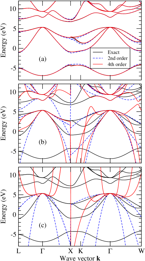
Figure 1: (Color online) Energy band structure of bulk Al_0.5Ga_0.5As: comparison of exact calculation with $O(k^{2})$ and $O(k^{4})$ $\mathbf{k}\cdot\mathbf{p}$ models. (a) 283-state $\mathbf{k}\cdot\mathbf{p}$ model; (b) 7-state $\mathbf{k}\cdot\mathbf{p}$ model; (c) 3-state $\mathbf{k}\cdot\mathbf{p}$ model.

Part (a) shows the results when all 283 states of the plane-wave basis are retained in the $\mathbf{k}\cdot\mathbf{p}$ Hamiltonian. Here it makes little difference whether the polynomials in the $\mathbf{k}\cdot\mathbf{p}$ Hamiltonian are terminated at order $k^{2}$ or $k^{4}$; both cases provide a good description throughout the Brillouin zone. In part (b), the set $\mathcal{A}=\{\Gamma_{15\mathrm{c}},\Gamma_{1\mathrm{c}},\Gamma_{15\mathrm{v}}\}$ contains 7 states (or 14 with spinFlatté et al. (1996); Pfeffer and Zawadzki (1996)). The description of the band structure is still accurate near $\Gamma$, although spurious solutions within the energy gap do occur for both the $O(k^{2})$ and $O(k^{4})$ $\mathbf{k}\cdot\mathbf{p}$ models.

Part (c) gives the results for $\mathcal{A}=\{\Gamma_{15\mathrm{v}}\}$. Here there are no spurious solutions in the $O(k^{2})$ effective-mass model, but the spurious solutions for the $O(k^{4})$ model occur at rather small wave vectors. The critical point at which the light-hole band has zero slope is about $\frac{1}{6}$ of the distance to the $X$ point. To prevent problems with spurious solutions, the envelope functions in a (001) superlattice should contain no Fourier components beyond this point. Yang and Chang (2005) Therefore, a superlattice with a period of 48 monolayers Foreman (2007a) was chosen as the standard test case, since this permits the inclusion of 9 envelope-function plane waves within the region $|k_{z}|\leq\tfrac{4}{48}(4\pi/a)=\tfrac{1}{6}(2\pi/a)$. Previous calculations on empirical pseudopotential models show that this is sufficient to achieve reasonably accurate results. Xia (1989); Wang et al. (1997); Wang and Zunger (1997, 1999)

The features shown in Fig. 1(c) have a direct analog in the Dirac equation for relativistic electrons, for which the dispersion relation is

$$E =\sqrt{p^{2}c^{2}+m^{2}c^{4}}$$ (21a)

$$=mc^{2}+\frac{p^{2}}{2m}-\frac{p^{4}}{8m^{3}c^{2}}+\cdots.$$ (21b)

Here the power series converges only when $|p|<mc$. If the series is terminated at order $p^{4}$, the slope of $E(p)$ changes sign at $p=\sqrt{2}mc$, which lies outside the region of validity of the power series. Although the convergence radius of Luttinger–Kohn perturbation theory for the $\mathbf{k}\cdot\mathbf{p}$ Hamiltonian is not known, one would expect it also to be of the same order of magnitude as the critical point where $E(k)$ changes sign. Therefore, it is reasonable to choose this as the cutoff for plane-wave expansions, Yang and Chang (2005) even though it may lie slightly outside the convergence radius of the perturbation power series.

The GaAs/Al_0.2Ga_0.8As material system historically provided one of the first direct comparisons between experiment and effective-mass theory in heterostructures. Dingle et al. (1974) Figure 2 shows the top 12 valence subbands in a (001) (GaAs)₂₄(Al_0.2Ga_0.8As)₂₄ superlattice.

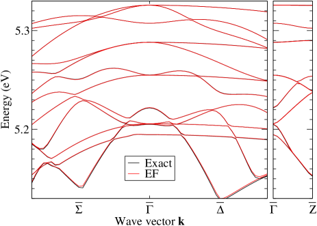
Figure 2: (Color online) Valence band structure of a (001) (GaAs)₂₄(Al_0.2Ga_0.8As)₂₄ superlattice: comparison of exact and 3-state envelope-function (EF) calculations. The EF model is the same as that of Ref. Foreman, 2005, and the calculation includes 9 plane waves (PW). Symmetry labels are defined in Refs. Sham and Lu, 1989 and Koster, 1957; the $\bar{\Sigma}$ axis corresponds to the bulk $\Delta$ axis, and the border of the figure in the $\bar{\Sigma}$ direction is 6% of the distance to the bulk $X$ point (the border in the $\bar{\Delta}$ or bulk $\Sigma$ direction is the same physical distance).

The exact model calculations are compared here with a 3-state $\Gamma_{15\mathrm{v}}$ envelope-function model based on the theory of Ref. Foreman, 2005, in which terms of order $k^{3}$ and $k^{4}$ are included only for the bulk reference crystal, the mass and momentum terms are linear in $\theta$, and the potential is quadratic in $\theta$. The envelope-function results are in excellent agreement with the exact calculations; the mean error in each of the first 10 subbands does not exceed 0.1 meV. Note that the valence-band offset in this system is only 104 meV, which means that the heterostructure perturbation is indeed shallow Kohn (1957) even in a single-band $\Gamma_{15\mathrm{v}}$ model. These results confirm that the theory of Ref. Foreman, 2005 works very well in the weak-perturbation limit under which it was derived.

The following examples provide a more detailed study of the effects of various approximations in systems containing stronger perturbations. Figure 3 shows the top 12 valence subbands in a (001) (GaAs)₂₄(AlAs)₂₄ superlattice.

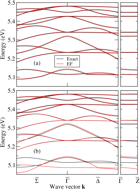
Figure 3: (Color online) Valence band structure of a (001) (GaAs)₂₄(AlAs)₂₄ superlattice: comparison of exact and 283-state EF calculations. (a) 25 EF plane waves; (b) 9 EF plane waves. Both EF calculations use $O(k^{4})$ bulk dispersion.

The exact model calculations are compared here with a 283-state envelope-function model that includes all zone-center Bloch functions explicitly, corresponding to Fig. 1(a) in the bulk case. Figure 3(a) includes 25 plane waves in the envelope-function model. The results here are very accurate, with an error corresponding to about a 2 meV shift that is nearly the same for all subbands. (To be more precise, the error in the ground state is $+1.6$ meV, which is almost the same as the $+1.5$ meV error in the bulk valence-band edge of GaAs calculated in Sec. VII C of the preceding paper.Foreman (2007a)) Figure 3(b) shows the effect of reducing the number of plane waves from 25 to 9. There is little change for energies close to the valence-band maximum, but the error in subband 12 is significant. Note that the energy range here is much wider than in Fig. 2, although it still corresponds approximately to the valence-band offset. Foreman (2007a)

The effect of reducing set $\mathcal{A}$ to the 7 states in $\Gamma_{15\mathrm{c}}$, $\Gamma_{1\mathrm{c}}$, and $\Gamma_{15\mathrm{v}}$ is shown in Fig. 4.

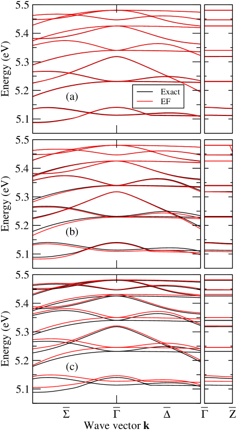
Figure 4: (Color online) Valence band structure of a (001) (GaAs)₂₄(AlAs)₂₄ superlattice: comparison of exact and 7-state EF calculations. The EF models are (a) $O(k^{4}\theta^{0}+k^{2}\theta^{1}+k^{0}\theta^{2})$; (b) $O(k^{2}\theta^{1}+k^{0}\theta^{2})$; (c) $O(k^{2}\theta^{0}+k^{0}\theta^{2})$. All EF calculations use 25 plane waves and $O(\theta^{2})$ potentials.

Part (a) is just the multiband theory of Ref. Foreman, 2005, the single-band version of which was used previously in Fig. 2. The results here are even slightly better than in Fig. 3(a), which can only be attributed to a fortuitous cancellation of errors. In part (b) the $O(k^{4}\theta^{0})$ terms are dropped. The results are still fairly accurate near the valence-band maximum; however, the peculiar behavior of (what should be) the ground state near $\bar{Z}$ shows that the plane-wave cutoff in this case is not quite sufficient to eliminate all effects of the $O(k^{2})$ spurious solutions in Fig. 1(b). In Fig. 4(c) the $O(k^{2}\theta^{1})$ terms are dropped, so that the mass and momentum matrices are approximated by those of the reference crystal. Here the error becomes significant even at fairly small energies, which shows the importance of including linear terms for multiband models.

In Figs. 5 and 6, the set $\mathcal{A}$ is reduced even further to only the three $\Gamma_{15\mathrm{v}}$ states.

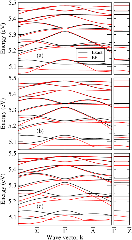
Figure 5: (Color online) Valence band structure of a (001) (GaAs)₂₄(AlAs)₂₄ superlattice: comparison of exact and 3-state EF calculations. The EF models are (a) $O(k^{4}\theta^{0}+k^{2}\theta^{1}+k^{0}\theta^{2})$, 9 PW; (b) $O(k^{4}\theta^{0}+k^{2}\theta^{2}+k^{0}\theta^{4})$, 9 PW; (c) $O(k^{2}\theta^{2}+k^{0}\theta^{4})$, 25 PW.

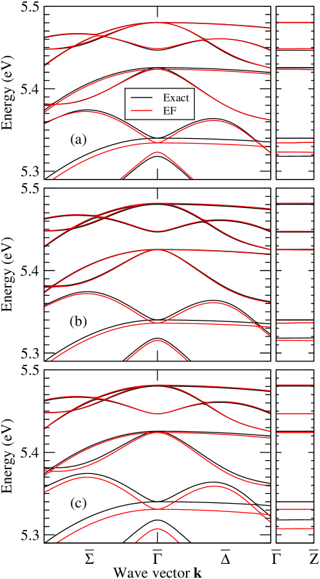
Figure 6: (Color online) Expanded view of the top eight valence states from Fig. 5.

Figure 5 shows the bands on the same energy scale as before, while Fig. 6 shows an expanded view of the region near the band edge. Part (a) uses the linear mass model of Ref. Foreman, 2005 (the same as in Fig. 2). A close inspection of the top three subbands in Fig. 6(a) shows evidence of the errors in the linear mass approximation displayed in Table 2. These errors are corrected in part (b), which includes quadratic corrections to the mass as well as (see Appendix E) terms of order $\theta^{4}$ in the potential. This yields a noticeable improvement, although the quantitative failure for higher excitations (due in large part to the use of only 9 plane waves) is still present. In part (c), the $O(k^{4}\theta^{0})$ terms are dropped; since spurious solutions are no longer a problem, the number of plane waves is increased to 25. It can be seen that the top three subbands are still quite accurate under this approximation.

Figure 7 shows the valence subband structure of a (001) (In_0.53Ga_0.47As)₂₄(InP)₂₄ superlattice.

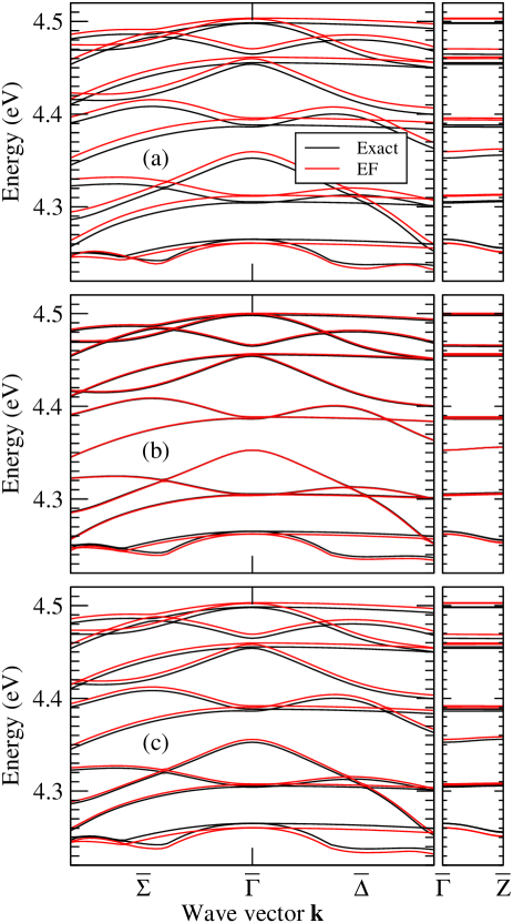
Figure 7: (Color online) Valence band structure of a (001) (In_0.53Ga_0.47As)₂₄(InP)₂₄ superlattice: comparison of exact and EF calculations. (a) 283-state EF model; (b) 7-state EF model, $O(k^{4}\theta^{0}+k^{2}\theta^{1}+k^{0}\theta^{2})$; (c) 7-state EF model, $O(k^{4}\theta^{0}+k^{2}\theta^{2}+k^{0}\theta^{4})$. All EF calculations use 25 plane waves and $O(k^{4})$ bulk dispersion.

Part (a) gives the results obtained from the original 283-state basis. The error here is larger than in the analogous calculation for GaAs/AlAs in Fig. 3(a); the ground-state error is $+5.1$ meV, which is close to the error of $+4.5$ meV in the bulk valence-band edge of In_0.53Ga_0.47As calculated in Sec. VII C of Ref. Foreman, 2007a. The deviation from a constant shift of about 5 meV is negligible for the first 10 subbands, which covers the full range of the valence-band offset. Foreman (2007a)

In Fig. 7(b) the basis is reduced to 7 states using the linear mass renormalization of Ref. Foreman, 2005. The results are quite close to the exact calculation, although again the improvement over part (a) is fortuitous. This is demonstrated in part (c), which includes additional terms of order $\theta^{2}k^{2}$ and $\theta^{4}k^{0}$. Most of the bands are shifted slightly upward, returning nearly to the result from part (a). The shift is mainly due to $O(\theta^{3}k^{0})$ corrections in the renormalized potential [see Eq. (48)]. Hence, neglecting $O(\theta^{3}k^{0})$ terms in perturbative renormalization [Fig. 7(b)] approximately compensates for the neglect of cubic response terms in the original Hamiltonian.

Figure 2 of Ref. Foreman, 2007b shows the results of calculations that are the same as Fig. 7(b), but for the 4-dimensional set $\mathcal{A}=\{\Gamma_{1\mathrm{c}},\Gamma_{15\mathrm{v}}\}$. The results with $O(\theta^{0}k^{4})$ terms are almost identical to Fig. 7(b). The effect of dropping the $O(\theta^{0}k^{4})$ terms is somewhat more significant than in Fig. 4(b), however.

Finally, Fig. 8 shows the predictions of the single-band $\Gamma_{15\mathrm{v}}$ model for In_0.53Ga_0.47As/InP.

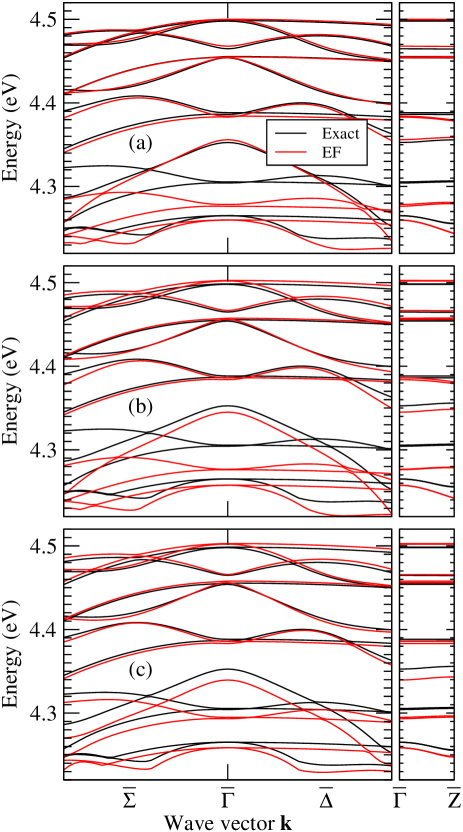
Figure 8: (Color online) Valence band structure of a (001) (In_0.53Ga_0.47As)₂₄(InP)₂₄ superlattice: comparison of exact and 3-state EF calculations. The EF models are (a) $O(k^{4}\theta^{0}+k^{2}\theta^{1}+k^{0}\theta^{2})$, 7 PW; (b) $O(k^{4}\theta^{0}+k^{2}\theta^{2}+k^{0}\theta^{4})$, 7 PW; (c) $O(k^{2}\theta^{2}+k^{0}\theta^{4})$, 25 PW.

When $O(k^{4})$ terms are included in the bulk Hamiltonian, the critical point of zero slope in the light-hole $\langle 100\rangle$ dispersion is closer to $\Gamma$ than it was in GaAs/AlAs, so that now only 7 plane waves can be included in the envelope functions if one wishes to avoid spurious solutions. Apart from this restriction, the envelope-function models used in parts (a), (b), and (c) of Fig. 8 are the same as those used in the corresponding parts of Figs. 5 and 6. It can be seen that in this case the limitations of using only 7 plane waves are sufficiently severe that, for the first seven subbands, one is better off omitting the $O(k^{4})$ terms and including more plane waves. It should be noted that the predictions of the single-band Hamiltonian for real In_0.53Ga_0.47As/InP superlattices would likely be substantially worse than what is shown here (perhaps even qualitatively incorrect), since the energy gap of In_0.53Ga_0.47As in the model system is 61% larger than the experimental value (see Sec. IV of the preceding paperForeman (2007a)).

Although it is not visible on the scale of these figures, the double degeneracy of the $\bar{\Gamma}$ ground state in GaAs/AlAs is removed in In_0.53Ga_0.47As/InP due to the reduction in symmetry from $D_{2d}$ to $C_{2v}$. The primary cause of the splitting is mixing of the $|X\rangle$ and $|Y\rangle$ valence states due to the short-range interface mixing in Eq. (17) and the long-range interface dipole potential in Fig. 10 of the preceding paper. Foreman (2007a) The splitting of the quasidegenerate ground state calculated exactly and in various envelope-function models is presented in Table 5.

Table 5: Splitting of the $\bar{\Gamma}$ ground-state degeneracy in a (001) (In_0.53Ga_0.47As)₂₄(InP)₂₄ superlattice.

Model	Diatomic dipole included?
	Yes	No
Exact	0.639 meV
EF (283 states)	0.722 meV
EF (7 states)	0.626 meV	0.426 meV
EF (3 states)	0.585 meV

It can be seen that all of the envelope-function models give a reasonably good estimate of the splitting (which means that they provide a satisfactory description of the microscopic wave function in the interface region). However, when the diatomic dipole terms in Fig. 10 of Ref. Foreman, 2007a (and their associated polarization of the bulk reference crystal) are omitted, the splitting of the ground state in the 7-dimensional envelope-function model is reduced by about one third. This shows that the practice of fitting experimental splitting data to short-range interface terms only Ivchenko et al. (1996); Lau and Flatté (2002); Szmulowicz et al. (2004) may give an incorrect description of the basic physics and overestimate the magnitude of the short-range terms.

VI Conclusions

This paper has presented a numerical implementation of the first-principles envelope-function theory of Ref. Foreman, 2005 in a model system based on superlattice LDA calculations with norm-conserving pseudopotentials. The electron density and potential energy of the superlattice were approximated by retaining only the linear and quadratic response to the heterostructure perturbation. This approximation worked well, with a net error of about 2 meV in GaAs/AlAs and 5 meV in In_0.53Ga_0.47As/InP. Foreman (2007a) The principal effect of this error was simply a constant shift of the superlattice energy eigenvalues.

The density and short-range potentials were then approximated further using truncated multipole expansions (i.e., power series in $k$), retaining terms of order $k^{2}$ in the linear potential and $k^{0}$ in the quadratic potential. This had no effect on the macroscopic density and potential in bulk, but it generated some additional error (due primarily to the truncation of the linear density response) in a narrow region near the interfaces. Foreman (2007a) This error was confirmed to be negligible for slowly varying envelope functions.

The approximate Hamiltonian was transformed from the original plane-wave basis to a Luttinger–Kohn basis using zone-center Bloch functions of the reference crystal. A Luttinger–Kohn unitary transformation was then used to eliminate the $\mathbf{k}\cdot\mathbf{p}$ and potential-energy coupling between the $\mathcal{A}$ states of interest and the remote $\mathcal{B}$ states. The resulting basis is material-dependent (due to the potential-energy terms) and approximates the position dependence of the quasi-Bloch functions in the heterostructure. The perturbation theory of Ref. Foreman, 2005 was extended to account for quadratic renormalization of the mass and momentum parameters.

A 7-state $\{\Gamma_{15\mathrm{v}},\Gamma_{1\mathrm{c}},\Gamma_{15\mathrm{c}}\}$ envelope-function model with linear momentum and mass renormalization was shown to give a very good description of the $\Gamma_{15}$ valence subband structure of GaAs/AlAs and In_0.53Ga_0.47As/InP (001) superlattices, although the good results were partly due to a fortuitous cancellation of errors. Calculations reported elsewhere Foreman (2007b) show that similar results for $\Gamma_{15\mathrm{v}}$ can be obtained from a simpler 4-state $\{\Gamma_{15\mathrm{v}},\Gamma_{1\mathrm{c}}\}$ model. A 3-state $\Gamma_{15\mathrm{v}}$ model gave fairly good results over a more limited energy range (although it probably would not work as well in real In_0.53Ga_0.47As/InP superlattices, since the energy gap of In_0.53Ga_0.47As in the model system was significantly greater than the experimental value). The primary limitation of this single-band model is a conflict between the need for $O(k^{4})$ bulk terms in order to achieve better accuracy in the excited states and the sometimes rather severe plane-wave cutoff needed to avoid spurious solutions generated by the $O(k^{4})$ terms. The 3-state model did, however, give excellent results for GaAs/Al_0.2Ga_0.8As, where the band offset is small enough to satisfy Kohn’s definition ($\lesssim 0.1$ eV)Kohn (1957) of a shallow perturbation.

Dipole terms in the quadratic response were found to produce interface asymmetry and macroscopic electric fields in the no-common-atom In_0.53Ga_0.47As/InP system. Foreman (2007a) These terms, which have $C_{2v}$ symmetry, produce a significant fraction of the splitting of the quasidegenerate ground state in such systems. Fitting this splitting to only short-range interface $XY$ mixing terms may therefore overestimate the short-range terms and omit important physics.

Numerical results for In_0.53Ga_0.47As/InP and GaAs/AlAs indicate that the linear valence-band Rashba coupling parameter is well approximated by the bulk effective Landé factor $K$ for cationic perturbations, but that there is a wide disparity for anionic perturbations. Therefore, using bulk magnetoabsorption measurements to evaluate interface parameters such as the Rashba coupling not (d); Rodina and Alekseev (2006) cannot generally be relied upon to provide anything better than a rough order-of-magnitude estimate. Of course, the particular numbers generated by the present model would likely change significantly in a more realistic quasiparticle calculation, but the discrepancy between the Rashba and Landé coefficients is unlikely to vanish.

The operator ordering of the effective-mass terms at a heterojunction was found to be more complicated than in many previous models. Instead of having a single von Roos kinetic-energy operator of the form shown in Eq. (1), perturbation theory yields a linear combination of terms with all possible operator orderings. Certain terms are larger than others, however. As shown by Leibler, Leibler (1975, 1977) to linear order only the BenDaniel–Duke operator BenDaniel and Duke (1966) $T_{\mathrm{BD}}=\tfrac{1}{2}pm^{-1}p$ and the Gora–Williams operator Gora and Williams (1969) $T_{\mathrm{GW}}=\tfrac{1}{4}(m^{-1}p^{2}+p^{2}m^{-1})$ arise. In a simple model where the matrix $E^{\alpha}_{nn^{\prime}}$ in Eq. (9) is assumed diagonal, the former arises in third-order perturbation theory from the position-dependent energies of remote bands in set $\mathcal{B}$, whereas the latter comes from the position dependence of the bands in set $\mathcal{A}$ (see Appendix D). The Zhu–Kroemer operator Zhu and Kroemer (1983) $T_{\mathrm{ZK}}=\tfrac{1}{2}m^{-1/2}p^{2}m^{-1/2}$ appears as one of several terms in quadratic renormalization, and the most general von Roos operator does not occur until cubic order.

Actually, with repeated use of the commutator $[p,f(z)]=-i(df/dz)$, one can move the momentum operators into any desired position. For example, Morrow and Brownstein have shown that, upon replacing $\alpha\rightarrow\alpha+\epsilon$ and $\gamma\rightarrow\alpha-\epsilon$ in Eq. (1), the von Roos operator can be rewritten as Morrow and Brownstein (1985)

$$T_{\mathrm{vR}}=T_{\mathrm{H}}-\frac{1}{2m}\left(\frac{d[\ln(m^{\epsilon})]}{dz}\right)^{2},$$ (22)

where $T_{\mathrm{H}}=\frac{1}{2}m^{\alpha}pm^{\beta}pm^{\alpha}$ is the Harrison operator Harrison (1961) and the second term has the form of a potential energy. But one can continue this process indefinitely, for example by writing

$$T_{\mathrm{H}}=T_{\mathrm{BD}}-\frac{d}{dz}\left(\frac{1}{2m}\frac{d[\ln(m^{\alpha})]}{dz}\right)+\frac{1}{2m}\left(\frac{d[\ln(m^{\alpha})]}{dz}\right)^{2}.$$ (23)

Hence, the operator ordering in the effective kinetic energy is nothing but an arbitrary convention, as long as one takes care to retain all of the effective potential-energy terms generated by changing conventions. Young (1989)

The effective kinetic-energy operator given by the perturbation theory in this paper does have the advantage that the position-dependent functions $\theta_{\alpha}(\mathbf{x})$ appearing in it are smooth step-like functions (although it should be noted that the position of the step is different for cations and anions). One could reduce it to the conventional BenDaniel–Duke form, or any other desired form, if one were willing to deal with functions having a more complicated position dependence near the interface.

This suggests that it may be possible—at least at the phenomenological level—to extend the perturbative scheme described here to arbitrarily high order in $\theta$. not (e) From this perspective, as long as (i) the bulk materials of the heterostructure are accurately described by an effective-mass equation and (ii) the heterostructure perturbation series eventually converges at some finite order, one can rearrange the operators into some standard order, yielding a standardized Hamiltonian with parameters that have a complicated but in principle calculable position dependence.

Of course, this is unlikely to provide a useful first-principles calculation method unless the series converges at a fairly low order. Fortunately, the examples given here demonstrate that linear (in the multiband case) or quadratic (in the single-band case) renormalization of the momentum and mass parameters is sufficient to achieve good results in several typical III-V heterostructures. Given that linear-response theory Baroni et al. (1989) has produced accurate predictions of valence-band offsets in many other lattice-matched and lattice-mismatched systems (see the bibliography of Ref. Foreman, 2005), it is likely that the present envelope-function theory can be applied successfully in many systems too.

Appendix A Nonlocal pseudopotential

The nonlocal part of the pseudopotential was handled by polynomial fitting in $\mathbf{k}$ space. For the bulk reference crystal, the entire plane-wave Hamiltonian matrix $H(\mathbf{k}+\mathbf{G},\mathbf{k}+\mathbf{G}^{\prime})\equiv H_{\mathbf{G}\mathbf{G}^{\prime}}(\mathbf{k})$ was evaluated at 57 points near $\mathbf{k}=\mathbf{0}$, including $\mathbf{k}=\mathbf{0}$ itself and points of the form $\langle 100\rangle$, $\langle 110\rangle$, $\langle 111\rangle$, $\langle 200\rangle$, and $\langle 210\rangle\times\Delta$, where $\Delta$ is some specified interval (usually set equal to half the magnitude of the smallest superlattice reciprocal-lattice vector). It is important to choose a set of fitting points with $O_{h}$ symmetry so that the fitted coefficients maintain the $T_{d}$ symmetry and time-reversal symmetry of the Hamiltonian. The Hamiltonian was fitted to a general polynomial of order $k^{4}$ with 35 independent coefficients. (For general $\mathbf{G}$ and $\mathbf{G}^{\prime}$, there is no special symmetry that can be used to reduce the number of coefficients.)

For the linear response, the nonlocal pseudopotential $V^{\mathrm{nl}}(\mathbf{k}+\mathbf{g},\mathbf{k}+\mathbf{g}^{\prime})$ may be written as $V^{\mathrm{nl}}_{\mathbf{G}\mathbf{G}^{\prime}}\bigl{(}k_{x},k_{y},k_{z}+\tfrac{1}{2}(\Delta g_{z}+\Delta g_{z}^{\prime}),\Delta g_{z}-\Delta g_{z}^{\prime}\bigr{)}$, in which $\mathbf{g}$ is a reciprocal-lattice vector of the superlattice and $\Delta\mathbf{g}\equiv\mathbf{g}-\mathbf{G}$ is an integer multiple of $(2\pi/Nd)\hat{\mathbf{z}}$, where $N$ is the number of monolayers in the superlattice. The function $V^{\mathrm{nl}}_{\mathbf{G}\mathbf{G}^{\prime}}(k_{1},k_{2},k_{3},k_{4})$ was fitted to a general polynomial of order $k^{2}$ with 15 independent coefficients using a set of 33 points arranged on a cubic grid. A larger grid was tested using fitting polynomials of order $k^{4}$, but the difference was negligible so only the simpler method was used. The nonlocal pseudopotential is purely linear, so no fitting of the quadratic response was necessary.

Appendix B Perturbation theory

This appendix defines a set of functions that offer a convenient way to describe operator ordering in fourth-order Luttinger–Kohn perturbation theory. These functions are merely an alternative way of writing the expressions given on p. 205 of Winkler’s monograph. Winkler (2003)

In Luttinger–Kohn perturbation theory, Luttinger and Kohn (1955); Bir and Pikus (1974) the total Hamiltonian of the system is written as $H=H_{0}+H^{\prime}$, where $H_{0}$ has matrix elements $(H_{0})_{mm^{\prime}}=E_{m}\delta_{mm^{\prime}}$. The states of the unperturbed Hamiltonian $H_{0}$ are divided into a set $\mathcal{A}$ containing the states of interest, and a set $\mathcal{B}$ containing all other states. It is assumed that the energies of $\mathcal{A}$ and $\mathcal{B}$ do not overlap. A unitary transformation $\bar{H}=e^{-S}He^{S}$ is used to eliminate the coupling between $\mathcal{A}$ and $\mathcal{B}$ to any desired order in the perturbation $H^{\prime}$.

The notation used here is defined as follows. $M_{\mathcal{AB}}$ is the block of the matrix $M$ that has rows in set $\mathcal{A}$ and columns in set $\mathcal{B}$. The matrix $G$ is defined by

$$(G_{\mathcal{AB}})_{nn^{\prime}} =(E_{n}-E_{n^{\prime}})^{-1}, G_{\mathcal{BA}} =(G_{\mathcal{AB}})^{\mathrm{T}},$$ (24)

where T denotes the transpose. A dot indicates element-by-element multiplication of congruent matrices:

$$(A\cdot B)_{nn^{\prime}}=A_{nn^{\prime}}B_{nn^{\prime}},$$ (25)

whereas juxtaposition denotes ordinary matrix multiplication.

The renormalized Hamiltonian $\bar{H}$ for states in $\mathcal{A}$ is given to fourth order in $H^{\prime}$ by Winkler (2003)

$$\bar{H}_{\mathcal{AA}}=H_{\mathcal{AA}}+P_{2}(H^{\prime},H^{\prime})+P_{3}(H^{\prime},H^{\prime},H^{\prime})\\ +P_{4}(H^{\prime},H^{\prime},H^{\prime},H^{\prime}),$$ (26)

where the functions $P_{2}$, $P_{3}$, and $P_{4}$ are defined by

$$P_{2}(H^{1},H^{2})=\tfrac{1}{2}[(H^{1}_{\mathcal{AB}}\cdot G_{\mathcal{AB}})H^{2}_{\mathcal{BA}}+H^{1}_{\mathcal{AB}}(G_{\mathcal{BA}}\cdot H^{2}_{\mathcal{BA}})],$$ (27)

$$P_{3}(H^{1},H^{2},H^{3})=\tfrac{1}{2}\{[(H^{1}_{\mathcal{AB}}\cdot G_{\mathcal{AB}})H^{2}_{\mathcal{BB}}]\cdot G_{\mathcal{AB}}\}H^{3}_{\mathcal{BA}}\\ +\tfrac{1}{2}H^{1}_{\mathcal{AB}}\{G_{\mathcal{BA}}\cdot[H^{2}_{\mathcal{BB}}(G_{\mathcal{BA}}\cdot H^{3}_{\mathcal{BA}})]\}\\ -\tfrac{1}{2}\{[H^{1}_{\mathcal{AA}}(G_{\mathcal{AB}}\cdot H^{2}_{\mathcal{AB}})]\cdot G_{\mathcal{AB}}\}H^{3}_{\mathcal{BA}}\\ -\tfrac{1}{2}H^{1}_{\mathcal{AB}}\{G_{\mathcal{BA}}\cdot[(H^{2}_{\mathcal{BA}}\cdot G_{\mathcal{BA}})H^{3}_{\mathcal{AA}}]\},$$ (28)

$$P_{4}(H^{1},H^{2},H^{3},H^{4})=\\ =\tfrac{1}{2}\bigl{[}\bigl{(}H^{1}_{\mathcal{AA}}\{G_{\mathcal{AB}}\cdot[H^{2}_{\mathcal{AA}}(G_{\mathcal{AB}}\cdot H^{3}_{\mathcal{AB}})]\}\bigr{)}\cdot G_{\mathcal{AB}}\bigr{]}H^{4}_{\mathcal{BA}}\\ +\tfrac{1}{2}H^{1}_{\mathcal{AB}}\bigl{[}G_{\mathcal{BA}}\cdot\bigl{(}\{[(H^{2}_{\mathcal{BA}}\cdot G_{\mathcal{BA}})H^{3}_{\mathcal{AA}}]\cdot G_{\mathcal{BA}}\}H^{4}_{\mathcal{AA}}\bigr{)}\bigr{]}\\ -\tfrac{1}{2}H^{1}_{\mathcal{AB}}\bigl{[}G_{\mathcal{BA}}\cdot\bigl{(}\{[H^{2}_{\mathcal{BB}}(G_{\mathcal{BA}}\cdot H^{3}_{\mathcal{BA}})]\cdot G_{\mathcal{BA}}\}H^{4}_{\mathcal{AA}}\bigr{)}\bigr{]}\\ -\tfrac{1}{2}H^{1}_{\mathcal{AB}}\bigl{[}G_{\mathcal{BA}}\cdot\bigl{(}H^{2}_{\mathcal{BB}}\{G_{\mathcal{BA}}\cdot[(H^{3}_{\mathcal{BA}}\cdot G_{\mathcal{BA}})H^{4}_{\mathcal{AA}}]\}\bigr{)}\bigr{]}\\ -\tfrac{1}{2}\bigl{[}\bigl{(}H^{1}_{\mathcal{AA}}\{G_{\mathcal{AB}}\cdot[(H^{2}_{\mathcal{AB}}\cdot G_{\mathcal{AB}})H^{3}_{\mathcal{BB}}]\}\bigr{)}\cdot G_{\mathcal{AB}}\bigr{]}H^{4}_{\mathcal{BA}}\\ -\tfrac{1}{2}\bigl{[}\bigl{(}\{[H^{1}_{\mathcal{AA}}(G_{\mathcal{AB}}\cdot H^{2}_{\mathcal{AB}})]\cdot G_{\mathcal{AB}}\}H^{3}_{\mathcal{BB}}\bigr{)}\cdot G_{\mathcal{AB}}\bigr{]}H^{4}_{\mathcal{BA}}\\ -\tfrac{1}{3}\bigl{(}\{[(H^{1}_{\mathcal{AB}}\cdot G_{\mathcal{AB}})H^{2}_{\mathcal{BA}}](G_{\mathcal{AB}}\cdot H^{3}_{\mathcal{AB}})\}\cdot G_{\mathcal{AB}}\bigr{)}H^{4}_{\mathcal{BA}}\\ -\tfrac{1}{3}H^{1}_{\mathcal{AB}}\bigl{(}G_{\mathcal{BA}}\cdot\{(H^{2}_{\mathcal{BA}}\cdot G_{\mathcal{BA}})[H^{3}_{\mathcal{AB}}(G_{\mathcal{BA}}\cdot H^{4}_{\mathcal{BA}})]\}\bigr{)}\\ -\tfrac{1}{6}\{[(H^{1}_{\mathcal{AB}}\cdot G_{\mathcal{AB}})(H^{2}_{\mathcal{BA}}\cdot G_{\mathcal{BA}})H^{3}_{\mathcal{AB}}]\cdot G_{\mathcal{AB}}\}H^{4}_{\mathcal{BA}}\\ -\tfrac{1}{6}\{[H^{1}_{\mathcal{AB}}(G_{\mathcal{BA}}\cdot H^{2}_{\mathcal{BA}})(G_{\mathcal{AB}}\cdot H^{3}_{\mathcal{AB}})]\cdot G_{\mathcal{AB}}\}H^{4}_{\mathcal{BA}}\\ -\tfrac{1}{6}H^{1}_{\mathcal{AB}}\{G_{\mathcal{BA}}\cdot[H^{2}_{\mathcal{BA}}(G_{\mathcal{AB}}\cdot H^{3}_{\mathcal{AB}})(G_{\mathcal{BA}}\cdot H^{4}_{\mathcal{BA}})]\}\\ -\tfrac{1}{6}H^{1}_{\mathcal{AB}}\{G_{\mathcal{BA}}\cdot[(H^{2}_{\mathcal{BA}}\cdot G_{\mathcal{BA}})(H^{3}_{\mathcal{AB}}\cdot G_{\mathcal{AB}})H^{4}_{\mathcal{BA}}]\}\\ +\tfrac{1}{24}(H^{1}_{\mathcal{AB}}\cdot G_{\mathcal{AB}})(H^{2}_{\mathcal{BA}}\cdot G_{\mathcal{BA}})(H^{3}_{\mathcal{AB}}\cdot G_{\mathcal{AB}})H^{4}_{\mathcal{BA}}\\ +\tfrac{1}{24}H^{1}_{\mathcal{AB}}(G_{\mathcal{BA}}\cdot H^{2}_{\mathcal{BA}})(G_{\mathcal{AB}}\cdot H^{3}_{\mathcal{AB}})(G_{\mathcal{BA}}\cdot H^{4}_{\mathcal{BA}})\\ +\tfrac{1}{8}(H^{1}_{\mathcal{AB}}\cdot G_{\mathcal{AB}})(H^{2}_{\mathcal{BA}}\cdot G_{\mathcal{BA}})H^{3}_{\mathcal{AB}}(G_{\mathcal{BA}}\cdot H^{4}_{\mathcal{BA}})\\ +\tfrac{1}{8}(H^{1}_{\mathcal{AB}}\cdot G_{\mathcal{AB}})H^{2}_{\mathcal{BA}}(G_{\mathcal{AB}}\cdot H^{3}_{\mathcal{AB}})(G_{\mathcal{BA}}\cdot H^{4}_{\mathcal{BA}})\\ +\tfrac{1}{2}\bigl{[}\bigl{(}\{[(H^{1}_{\mathcal{AB}}\cdot G_{\mathcal{AB}})H^{2}_{\mathcal{BB}}]\cdot G_{\mathcal{AB}}\}H^{3}_{\mathcal{BB}}\bigr{)}\cdot G_{\mathcal{AB}}\bigr{]}H^{4}_{\mathcal{BA}}\\ +\tfrac{1}{2}H^{1}_{\mathcal{AB}}\bigl{[}G_{\mathcal{BA}}\cdot\bigl{(}H^{2}_{\mathcal{BB}}\{G_{\mathcal{BA}}\cdot[H^{3}_{\mathcal{BB}}(G_{\mathcal{BA}}\cdot H^{4}_{\mathcal{BA}})]\}\bigr{)}\bigr{]}.$$ (29)

This way of expressing $\bar{H}_{\mathcal{AA}}$ is particularly useful when $H^{\prime}$ is a sum of operators that do not commute, and one wishes to keep track of the order of the various terms. In the present case, $H^{\prime}$ is a sum of $\mathbf{k}\cdot\mathbf{p}$ terms and potential-energy matrix elements. Examples are given in the appendices below.

Appendix C Bulk renormalization

In terms of the functions defined in Appendix B, the renormalized coefficients of order $k^{2}$, $k^{3}$, and $k^{4}$ in the bulk reference Hamiltonian for set $\mathcal{A}$ are given by Foreman (2005)

$$D^{ij}_{\mathcal{AA}}=\tilde{D}^{ij}_{\mathcal{AA}}+P_{2}(\pi^{i},\pi^{j}),$$ (30)

$$C^{ijk}_{\mathcal{AA}}=\tilde{C}^{ijk}_{\mathcal{AA}}+P_{2}(\pi^{i},\tilde{D}^{jk})+P_{2}(\tilde{D}^{ij},\pi^{k})+P_{3}(\pi^{i},\pi^{j},\pi^{k}),$$ (31)

$$Q^{ijkl}_{\mathcal{AA}}=\tilde{Q}^{ijkl}_{\mathcal{AA}}+P_{4}(\pi^{i},\pi^{j},\pi^{k},\pi^{l})\\ +P_{3}(\tilde{D}^{ij},\pi^{k},\pi^{l})+P_{3}(\pi^{i},\tilde{D}^{jk},\pi^{l})+P_{3}(\pi^{i},\pi^{j},\tilde{D}^{kl})\\ +P_{2}(\tilde{D}^{ij},\tilde{D}^{kl})+P_{2}(\pi^{i},\tilde{C}^{jkl})+P_{2}(\tilde{C}^{ijk},\pi^{l}).$$ (32)

Here a tilde denotes a quantity before renormalization, which is obtained by fitting the reference Hamiltonian to a polynomial of order $k^{4}$ (as described in Appendix A). The tilde is omitted on $\pi^{i}$ because it does not change under renormalization.

Appendix D Linear renormalization

The terms in the renormalized $\mathcal{A}$ Hamiltonian that are linear in $\theta_{\alpha}$ are given by Foreman (2005)

$$\pi^{i\alpha}_{\mathcal{AA}} =\tilde{\pi}^{i\alpha}_{\mathcal{AA}}+P_{2}(\pi^{i},E^{\alpha}),$$ (33)

$$\pi^{\alpha i}_{\mathcal{AA}} =\tilde{\pi}^{\alpha i}_{\mathcal{AA}}+P_{2}(E^{\alpha},\pi^{i}),$$ (34)

$$D^{\alpha ij}_{\mathcal{AA}}=\tilde{D}^{\alpha ij}_{\mathcal{AA}}+P_{2}(\tilde{\pi}^{\alpha i},\pi^{j})+P_{2}(E^{\alpha},\tilde{D}^{ij})\\ +P_{3}(E^{\alpha},\pi^{i},\pi^{j}),$$ (35)

$$D^{i\alpha j}_{\mathcal{AA}}=\tilde{D}^{i\alpha j}_{\mathcal{AA}}+P_{2}(\tilde{\pi}^{i\alpha},\pi^{j})+P_{2}(\pi^{i},\tilde{\pi}^{\alpha j})\\ +P_{3}(\pi^{i},E^{\alpha},\pi^{j}),$$ (36)

$$D^{ij\alpha}_{\mathcal{AA}}=\tilde{D}^{ij\alpha}_{\mathcal{AA}}+P_{2}(\pi^{i},\tilde{\pi}^{j\alpha})+P_{2}(\tilde{D}^{ij},E^{\alpha})\\ +P_{3}(\pi^{i},\pi^{j},E^{\alpha}).$$ (37)

These are the same as the expressions given in Appendix C of Ref. Foreman, 2005, although written in a different notation. Once again, a tilde denotes a quantity before renormalization, which is obtained from a multipole expansion of the linear density and short-range potentials (Sec. II and Ref. Foreman, 2007a) and from fitting the linear nonlocal potential to a polynomial of order $k^{2}$ (Appendix A). The tilde is omitted on $E^{\alpha}$ because it does not change under renormalization.

Appendix E Quadratic renormalization

Perturbative renormalization also generates terms that are quadratic in $\theta_{\alpha}$. The only term included in the Hamiltonian of Ref. Foreman, 2005 was the renormalized potential

$$E^{\alpha\beta}_{\mathcal{AA}}=P_{2}(E^{\alpha},E^{\beta}).$$ (38)

Some of the present calculations also include quadratic renormalization of the momentum matrix:

$$\pi^{\alpha\beta i}_{\mathcal{AA}}=P_{2}(E^{\alpha},\tilde{\pi}^{\beta i})+P_{2}(\tilde{E}^{\alpha\beta},\pi^{i})+P_{3}(E^{\alpha},E^{\beta},\pi^{i}),$$ (39)

$$\pi^{\alpha i\beta}_{\mathcal{AA}}=P_{2}(E^{\alpha},\tilde{\pi}^{i\beta})+P_{2}(\tilde{\pi}^{\alpha i},E^{\beta})+P_{3}(E^{\alpha},\pi^{i},E^{\beta}),$$ (40)

$$\pi^{i\alpha\beta}_{\mathcal{AA}}=P_{2}(\tilde{\pi}^{i\alpha},E^{\beta})+P_{2}(\pi^{i},\tilde{E}^{\alpha\beta})+P_{3}(\pi^{i},E^{\alpha},E^{\beta}),$$ (41)

and of the effective masses:

$$D^{\alpha\beta ij}_{\mathcal{AA}}=P_{2}(E^{\alpha},\tilde{D}^{\beta ij})+P_{2}(\tilde{E}^{\alpha\beta},\tilde{D}^{ij})\\ +P_{3}(E^{\alpha},E^{\beta},\tilde{D}^{ij})+P_{3}(E^{\alpha},\tilde{\pi}^{\beta i},\pi^{j})+P_{3}(\tilde{E}^{\alpha\beta},\pi^{i},\pi^{j})\\ +P_{4}(E^{\alpha},E^{\beta},\pi^{i},\pi^{j}),$$ (42)

$$D^{i\alpha\beta j}_{\mathcal{AA}}=P_{2}(\tilde{\pi}^{i\alpha},\tilde{\pi}^{\beta j})+P_{3}(\tilde{\pi}^{i\alpha},E^{\beta},\pi^{j})\\ +P_{3}(\pi^{i},E^{\alpha},\tilde{\pi}^{\beta j})+P_{3}(\pi^{i},\tilde{E}^{\alpha\beta},\pi^{j})\\ +P_{4}(\pi^{i},E^{\alpha},E^{\beta},\pi^{j}),$$ (43)

$$D^{ij\alpha\beta}_{\mathcal{AA}}=P_{2}(\tilde{D}^{ij\alpha},E^{\beta})+P_{2}(\tilde{D}^{ij},\tilde{E}^{\alpha\beta})\\ +P_{3}(\tilde{D}^{ij},E^{\alpha},E^{\beta})+P_{3}(\pi^{i},\tilde{\pi}^{j\alpha},E^{\beta})+P_{3}(\pi^{i},\pi^{j},\tilde{E}^{\alpha\beta})\\ +P_{4}(\pi^{i},\pi^{j},E^{\alpha},E^{\beta}),$$ (44)

$$D^{\alpha i\beta j}_{\mathcal{AA}}=P_{2}(\tilde{\pi}^{\alpha i},\tilde{\pi}^{\beta j})+P_{2}(E^{\alpha},\tilde{D}^{i\beta j})\\ +P_{3}(E^{\alpha},\pi^{i},\tilde{\pi}^{\beta j})+P_{3}(E^{\alpha},\tilde{\pi}^{i\beta},\pi^{j})+P_{3}(\tilde{\pi}^{\alpha i},E^{\beta},\pi^{j})\\ +P_{4}(E^{\alpha},\pi^{i},E^{\beta},\pi^{j}),$$ (45)

$$D^{i\alpha j\beta}_{\mathcal{AA}}=P_{2}(\tilde{\pi}^{i\alpha},\tilde{\pi}^{j\beta})+P_{2}(\tilde{D}^{i\alpha j},E^{\beta})\\ +P_{3}(\tilde{\pi}^{i\alpha},\pi^{j},E^{\beta})+P_{3}(\pi^{i},\tilde{\pi}^{\alpha j},E^{\beta})+P_{3}(\pi^{i},E^{\alpha},\tilde{\pi}^{j\beta})\\ +P_{4}(\pi^{i},E^{\alpha},\pi^{j},E^{\beta}),$$ (46)

$$D^{\alpha ij\beta}_{\mathcal{AA}}=P_{2}(\tilde{\pi}^{\alpha i},\tilde{\pi}^{j\beta})+P_{2}(\tilde{D}^{\alpha ij},E^{\beta})+P_{2}(E^{\alpha},\tilde{D}^{ij\beta})\\ +P_{3}(\tilde{\pi}^{\alpha i},\pi^{j},E^{\beta})+P_{3}(E^{\alpha},\tilde{D}^{ij},E^{\beta})+P_{3}(E^{\alpha},\pi^{i},\tilde{\pi}^{j\beta})\\ +P_{4}(E^{\alpha},\pi^{i},\pi^{j},E^{\beta}).$$ (47)

In these expressions, several approximations are used. No fitting of the momentum and mass terms in the original quadratic Hamiltonian was performed here; consequently, the unrenormalized parts are set to zero. Also, the term $\tilde{E}^{\alpha\beta}$ is the mean unrenormalized diatomic short-range potential summed over all diatomic perturbations with the given values of $\alpha$ and $\beta$.

Some of the calculations also include renormalized short-range potential terms of order $\theta^{3}$ and $\theta^{4}$, which were approximated using the expressions

$$E^{\alpha\beta\gamma}_{\mathcal{AA}}=P_{2}(\tilde{E}^{\alpha\beta},E^{\gamma})+P_{2}(E^{\alpha},\tilde{E}^{\beta\gamma})+P_{3}(E^{\alpha},E^{\beta},E^{\gamma}),$$ (48)

$$E^{\alpha\beta\gamma\delta}_{\mathcal{AA}}=P_{2}(\tilde{E}^{\alpha\beta},\tilde{E}^{\gamma\delta})+P_{3}(E^{\alpha},E^{\beta},\tilde{E}^{\gamma\delta})\\ +P_{3}(E^{\alpha},\tilde{E}^{\beta\gamma},E^{\delta})+P_{3}(\tilde{E}^{\alpha\beta},E^{\gamma},E^{\delta})\\ +P_{4}(E^{\alpha},E^{\beta},E^{\gamma},E^{\delta}).$$ (49)

Corrections of the same order arising from the long-range terms in the Hartree potential were neglected. For all of the numerical examples treated here, the $O(\theta^{4})$ terms in Eq. (49) were found to be negligible.

It should be emphasized that the results presented here do not provide a fully consistent perturbation scheme according to the criteria given by Takhtamirov and Volkov, Takhtamirov and Volkov (1999) in which the mean kinetic energy of the states of interest is assumed to be comparable to the heterostructure potential-energy perturbation. According to this scheme, if one includes the $O(k^{2}\theta^{2})$ and $O(k^{0}\theta^{3})$ terms shown here, one should also include terms of order $k^{4}\theta^{1}$ and $k^{6}\theta^{0}$.

However, since these require the use of sixth-order perturbation theory, such terms were judged to be not worth the effort in a preliminary investigation of this nature. Therefore, the results obtained by adding only the $O(k^{2}\theta^{2})$ and $O(k^{0}\theta^{3})$ terms are not expected to be valid for kinetic energies covering the full range of the band offset, but only for kinetic energies small in comparison to the band offset. This is indeed what was found in the numerical calculations of Sec. V. Likewise, the $O(k^{4}\theta^{0})$ terms were found to be less important for states of small kinetic energy. These results are merely a reflection of the fact that a wide quantum well, unlike a hydrogenic impurity, Bir and Pikus (1974) does have states in which the mean kinetic energy is small compared to the mean perturbing potential. Thus, in this sense the theory of low-energy excitations of wide quantum wells is actually simpler than the corresponding theory of shallow impurities, because terms of high order in $k$ are of lesser importance.

Appendix F Quadratic response

The method used here to handle the quadratic response differs slightly from that of Ref. Foreman, 2005. The quadratic potential response is given by Eq. (3.14) of Ref. Foreman, 2005:

$$V^{(2)}(\mathbf{x},\mathbf{x}^{\prime})=\sideset{}{{}^{\prime}}{\sum}_{\alpha,\mathbf{R}}\sideset{}{{}^{\prime}}{\sum}_{\alpha^{\prime},\mathbf{R}^{\prime}}\theta^{\alpha}_{\mathbf{R}}\theta^{\alpha^{\prime}}_{\mathbf{R}^{\prime}}\Delta v^{\alpha\alpha^{\prime}}_{\mathbf{R}\mathbf{R}^{\prime}}(\mathbf{x},\mathbf{x}^{\prime}),$$ (50)

which has the same form as the quadratic density response in Eq. (3c). The translation symmetry of the reference crystal allows $\Delta v^{\alpha\alpha^{\prime}}_{\mathbf{R}\mathbf{R}^{\prime}}(\mathbf{x},\mathbf{x}^{\prime})$ to be written as

$$\Delta v^{\alpha\alpha^{\prime}}_{\mathbf{R}\mathbf{R}^{\prime}}(\mathbf{x},\mathbf{x}^{\prime})\equiv\Delta v^{\alpha\alpha^{\prime},\mathbf{R}^{\prime}-\mathbf{R}}(\mathbf{x}-\bar{\mathbf{R}}_{\alpha\alpha^{\prime}},\mathbf{x}^{\prime}-\bar{\mathbf{R}}_{\alpha\alpha^{\prime}}),$$ (51)

in which $\bar{\mathbf{R}}_{\alpha\alpha^{\prime}}$ is the midpoint of the two atoms:

$$\bar{\mathbf{R}}_{\alpha\alpha^{\prime}}=\tfrac{1}{2}(\mathbf{R}+\mathbf{R}^{\prime}+\bm{\tau}_{\alpha}+\bm{\tau}_{\alpha^{\prime}}).$$ (52)

In Eq. (51), the coordinate reference is taken to be $\bar{\mathbf{R}}_{\alpha\alpha^{\prime}}$, whereas in Eq. (3.17) of Ref. Foreman, 2005, it was chosen to be $\mathbf{R}_{\alpha}\equiv\mathbf{R}+\bm{\tau}_{\alpha}$. The Fourier transform of Eq. (50) is Foreman (2005)

$$V^{(2)}(\mathbf{k},\mathbf{k}^{\prime})=N\sideset{}{{}^{\prime}}{\sum}_{\alpha,\alpha^{\prime},\mathbf{R}^{\prime}}\theta^{\alpha\alpha^{\prime}\mathbf{R}^{\prime}}(\mathbf{k}-\mathbf{k}^{\prime})\Delta v^{\alpha\alpha^{\prime}\mathbf{R}^{\prime}}(\mathbf{k},\mathbf{k}^{\prime}),$$ (53)

where

$$\theta^{\alpha\alpha^{\prime}\mathbf{R}^{\prime}}(\mathbf{k})=\frac{1}{N}\sum_{\mathbf{R}}\theta^{\alpha}_{\mathbf{R}}\theta^{\alpha^{\prime}}_{\mathbf{R}+\mathbf{R}^{\prime}}e^{-i\mathbf{k}\cdot[\mathbf{R}_{\alpha}+(\mathbf{R}^{\prime}+\bm{\tau}_{\alpha^{\prime}}-\bm{\tau}_{\alpha})/2]}.$$ (54)

The coordinate reference (52) is arbitrary, but it is sometimes more convenient for analyzing symmetry properties than the choice used in Ref. Foreman, 2005.

In the LDA model used here, the quadratic potential is local [i.e., $\Delta v^{\alpha\alpha^{\prime}\mathbf{R}^{\prime}}(\mathbf{k},\mathbf{k}^{\prime})=\Delta v^{\alpha\alpha^{\prime}\mathbf{R}^{\prime}}(\mathbf{k}-\mathbf{k}^{\prime})$] since the ionic pseudopotential is purely linear. The diatomic potential $\Delta v^{\alpha\alpha^{\prime}\mathbf{R}^{\prime}}(\mathbf{q})$ was approximated for small $\mathbf{q}$ by keeping only the dipole and quadrupole terms in the electron density and the $l=0$ term in the power-series expansion (4) of the short-range potential (which in the quadratic case consists only of the exchange-correlation potential). For $\mathbf{q}$ near $\mathbf{G}\neq\mathbf{0}$, only the $l=0$ terms were retained in both the density and short-range potential; see Sec. VI B of the preceding paper Foreman (2007a) for further details.

References

- Foreman (2005) B. A. Foreman, Phys. Rev. B 72, 165345 (2005).
- Foreman (2007a) B. A. Foreman (2007a), eprint [arXiv]cond-mat/0703697.
- Luttinger and Kohn (1955) J. M. Luttinger and W. Kohn, Phys. Rev. 97, 869 (1955).
- Kohn (1957) W. Kohn, in Solid State Physics, edited by F. Seitz and D. Turnbull (Academic, New York, 1957), vol. 5, pp. 257–320.
- Bassani et al. (1974) F. Bassani, G. Iadonisi, and B. Preziosi, Rep. Prog. Phys. 37, 1099 (1974).
- Pantelides (1978) S. T. Pantelides, Rev. Mod. Phys. 50, 797 (1978).
- Sham (1966) L. J. Sham, Phys. Rev. 150, 720 (1966).
- Bir and Pikus (1974) G. L. Bir and G. E. Pikus, Symmetry and Strain-Induced Effects in Semiconductors (Wiley, New York, 1974); see §27 for corrections to elementary effective-mass theory.
- Burt (1992) M. G. Burt, J. Phys.: Condens. Matter 4, 6651 (1992).
- Takhtamirov and Volkov (1999) É. E. Takhtamirov and V. A. Volkov, JETP 89, 1000 (1999).
- Xia (1989) J.-B. Xia, Phys. Rev. B 39, 3310 (1989).
- Wang et al. (1997) L.-W. Wang, A. Franceschetti, and A. Zunger, Phys. Rev. Lett. 78, 2819 (1997).
- Wang and Zunger (1997) L.-W. Wang and A. Zunger, Phys. Rev. B 56, 12395 (1997).
- Wang and Zunger (1999) L.-W. Wang and A. Zunger, Phys. Rev. B 59, 15806 (1999).
- Keldysh (1964) L. V. Keldysh, Sov. Phys. JETP 18, 253 (1964).
- Leibler (1975) L. Leibler, Phys. Rev. B 12, 4443 (1975).
- Leibler (1977) L. Leibler, Phys. Rev. B 16, 863 (1977).
- Foreman (2007b) B. A. Foreman (2007b), eprint [arXiv]cond-mat/0612640.
- von Roos (1983) O. von Roos, Phys. Rev. B 27, 7547 (1983).
- Morrow and Brownstein (1984) R. A. Morrow and K. R. Brownstein, Phys. Rev. B 30, 678 (1984).
- Morrow and Brownstein (1985) R. A. Morrow and K. R. Brownstein, Phys. Rev. B 31, 1135 (1985).
- Gora and Williams (1969) T. Gora and F. Williams, Phys. Rev. 177, 1179 (1969).
- Payne et al. (1992) M. C. Payne, M. P. Teter, D. C. Allan, T. A. Arias, and J. D. Joannopoulos, Rev. Mod. Phys. 64, 1045 (1992).
- Martin (2004) R. M. Martin, Electronic Structure: Basic Theory and Practical Methods (Cambridge University Press, Cambridge, 2004).
- Gonze et al. (2002) X. Gonze et al., Comput. Mater. Sci. 25, 478 (2002).
- Gonze et al. (2005) X. Gonze et al., Z. Kristallogr. 220, 558 (2005).
- (27) The abinit code is a common project of the Université Catholique de Louvain, Corning Incorporated, and other contributors (URL http://www.abinit.org).
- Winkler (2003) R. Winkler, Spin-Orbit Coupling Effects in Two-Dimensional Electron and Hole Systems, vol. 191 of Springer Tracts in Modern Physics (Springer, Berlin, 2003).
- Luttinger (1956) J. M. Luttinger, Phys. Rev. 102, 1030 (1956).
- not (a) If one considers single atomic perturbations rather than planar perturbations, there are additional nonanalytic contributions from the linear octopole and hexadecapole moments of the electron density.Foreman (2005) For the present case of planar perturbations, these are simply absorbed into the definition of the short-range potential using Eq. (12) of Ref. Foreman, 2007a.
- not (b) For examples illustrating the transformation of operators from momentum to coordinate space, see Eqs. (22.10b) and (22.14c) of Bir and Pikus Bir and Pikus (1974) and Eqs. (4.7) and (4.8) of Winkler.Winkler (2003)
- Ivchenko et al. (1996) E. L. Ivchenko, A. Yu. Kaminski, and U. Rössler, Phys. Rev. B 54, 5852 (1996).
- Lin-Liu and Sham (1985) Y. R. Lin-Liu and L. J. Sham, Phys. Rev. B 32, R5561 (1985).
- Eppenga et al. (1987) R. Eppenga, M. F. H. Schuurmans, and S. Colak, Phys. Rev. B 36, 1554 (1987).
- Rashba (1960) É. I. Rashba, Sov. Phys. Solid State 2, 1109 (1960).
- Bychkov and Rashba (1984) Yu. A. Bychkov and E. I. Rashba, J. Phys. C 17, 6039 (1984).
- Winkler (2000) R. Winkler, Phys. Rev. B 62, 4245 (2000).
- Winkler et al. (2002) R. Winkler, H. Noh, E. Tutuc, and M. Shayegan, Phys. Rev. B 65, 155303 (2002).
- Foreman (1993) B. A. Foreman, Phys. Rev. B 48, R4964 (1993).
- Pidgeon and Brown (1966) C. R. Pidgeon and R. N. Brown, Phys. Rev. 146, 575 (1966).
- Foreman (2006) B. A. Foreman, J. Phys.: Condens. Matter 18, 1335 (2006).
- not (c) They could be obtained from analytical derivatives of the nonlocal pseudopotential in space, but that was not done here since the primary focus of this paper is the physics of abrupt heterojunctions. The value of also depends on the choice of coupling between the nonlocal potential and the magnetic field.Foreman (2006)
- Kane (1980) E. O. Kane, in Narrow Gap Semiconductors: Physics and Applications, edited by W. Zawadzki (Springer, Berlin, 1980), vol. 133 of Lecture Notes in Physics, pp. 13–31.
- BenDaniel and Duke (1966) D. J. BenDaniel and C. B. Duke, Phys. Rev. 152, 683 (1966).
- Bastard (1988) G. Bastard, Wave Mechanics Applied to Semiconductor Heterostructures (Wiley, New York, 1988).
- Löwdin (1951) P.-O. Löwdin, J. Chem. Phys. 19, 1396 (1951).
- Flatté et al. (1996) M. E. Flatté, P. M. Young, L.-H. Peng, and H. Ehrenreich, Phys. Rev. B 53, 1963 (1996).
- Pfeffer and Zawadzki (1996) P. Pfeffer and W. Zawadzki, Phys. Rev. B 53, 12813 (1996).
- Yang and Chang (2005) W. Yang and K. Chang, Phys. Rev. B 72, 233309 (2005).
- Dingle et al. (1974) R. Dingle, W. Wiegmann, and C. H. Henry, Phys. Rev. Lett. 33, 827 (1974).
- Sham and Lu (1989) L. J. Sham and Y.-T. Lu, J. Lumin. 44, 207 (1989).
- Koster (1957) G. F. Koster, in Solid State Physics, edited by F. Seitz and D. Turnbull (Academic, New York, 1957), vol. 5, pp. 173–256.
- Lau and Flatté (2002) W. H. Lau and M. E. Flatté, Appl. Phys. Lett. 80, 1683 (2002).
- Szmulowicz et al. (2004) F. Szmulowicz, H. Haugan, and G. J. Brown, Phys. Rev. B 69, 155321 (2004).
- not (d) Rodina and Alekseev Rodina and Alekseev (2006) have suggested dividing the heterostructure Hamiltonian into a bulk part and a surface part, in which the valence-band Rashba parameters for the bulk part are defined to be the same as the magnetic Luttinger parameters. However, since by symmetry the surface part contains terms with the same mathematical structure as the bulk part, this division does not carry any meaning unless one can make some definite statement about the magnitude of the surface part. As shown by the model calculations presented here, the surface part in this scheme is not generally negligible.
- Rodina and Alekseev (2006) A. V. Rodina and A. Yu. Alekseev, Phys. Rev. B 73, 115312 (2006).
- Zhu and Kroemer (1983) Q.-G. Zhu and H. Kroemer, Phys. Rev. B 27, 3519 (1983).
- Harrison (1961) W. A. Harrison, Phys. Rev. 123, 85 (1961).
- Young (1989) K. Young, Phys. Rev. B 39, 13434 (1989).
- not (e) This scheme would be limited to the low-energy excitations of a wide quantum well or superlattice, as discussed in the remarks at the end of Appendix E.
- Baroni et al. (1989) S. Baroni, R. Resta, A. Baldereschi, and M. Peressi, in Spectroscopy of Semiconductor Microstructures, edited by G. Fasol, A. Fasolino, and P. Lugli (Plenum, New York, 1989), vol. 206 of NATO ASI Series B, pp. 251–272.