Two-magnon excitations in resonant inelastic x-ray scattering from quantum Heisenberg antiferromagnets

Abstract

We study two-magnon spectra in resonant inelastic x-ray scattering (RIXS) from the Heisenberg antiferromanets by extending the formula of Nomura and Igarashi (Phys. Rev. B 71, 035110 (2005)). The core-hole potential in the intermediate state of RIXS gives rise to a change in the exchange coupling between $3d$ electrons, leading to an effective interaction between the core hole and spins of $3d$ electrons. We derive a formula suitable to calculate the two-magnon RIXS intensities, replacing the bare core-hole potential responsible to charge excitations by this effective interaction creating two magnons in our previous formula. It consists of two factors, one of which determines the incident-photon-energy dependence and another is the two-magnon correlation function. We evaluate the former factor for La₂CuO₄ in terms of the density of states of the $4p$ states obtained by the band calculation. We also calculate the two-magnon correlation function as a function of energy loss $\omega$ and momentum transfer q of the Heisenberg model on a square lattice, by summing up the ladder diagrams after transforming the magnon-magnon interaction into a separable form. The calculated spectra form a broad peak around $\omega=3J$ for $S=1/2$ on the magnetic Brillouin zone boundary and vanish at $\textbf{q}=(0,0)$ and $(\pi,\pi)$. Such momentum dependence of the RIXS spectra could provide an excellent opportunity to study the dynamics in the Heisenberg model.

I Introduction

Resonant inelastic x-ray scattering (RIXS) has recently attracted much interest, since it provides valuable information of charge excitations in solids. -C. Kao et al. (1996); Hill et al. (1998); Hasan et al. (2000); Kim et al. (2002); Inami et al. (2003); Kim et al. (2004); Suga et al. (2005) Unlike optical measurement, it can probe directly the momentum dependence of the excitations. The $K$-edge resonance in transition-metal compounds is particularly useful, because the corresponding x-ray wavelengths are an order of lattice spacing. In this situation, the $1s$ core electron is prompted to an empty $4p$ state by absorbing photon, then charge excitations are created in order to screen the core-hole potential, and finally the photo-excited $4p$ electron is recombined with the core hole by emitting photon. In the end, charge excitations are left with energy and momentum transferred from photons.

For analyzing such spectra, Nomura and Igarashi (NI) have developed a formalism Nomura and Igarashi (2004, 2005); Igarashi et al. (2006) by adapting the resonant Raman theory of Nozières and Abrahams. Nozières and Abrahams (1974) According to the formula NI have derived, the RIXS intensity is expressed in terms of the density-density correlation function in the equilibrium system under the Born approximation to the core-hole potential. Describing the electronic states on the multiband tight-binding model within the Hartree-Fock approximation, and taking account of the electron correlation within the random phase approximation, Nomura and Igarashi have analyzed the RIXS spectra of undoped cuprates. Nomura and Igarashi (2004, 2005); Igarashi et al. (2006) The calculated spectra have reproduced well the experimental ones as a function of energy loss and the dependence on momentum. The use of the Born approximation to the core-hole potential has been examined by evaluating higher-order corrections, and have partly been justified in spite of a strong core-hole potential.Igarashi et al. (2006) In addition, the RIXS spectra in NiO have recently been analyzed by the same method, in an excellent agreement with the experiment. Takahashi et al. Therefore, the NI formula seems quite useful to analyze the RIXS spectra. Note that most theoretical studies on the momentum dependence of the RIXS spectra have been based on the numerical diagonalization method for small clusters with replacing the $4p$ band by a single level. Tsutsui et al. (1999); Okada and Kotani (2006) By these numerical methods, it seems practically impossible to analyze the RIXS spectra in three dimensional systems.

Quite recently, Hill et al. have reported that the RIXS intensity has been observed around the energy loss $300\sim 600$ meV in La₂CuO₄ with improving the instrumental resolution.Com One scenario for the origin of the spectra is that the intensity arises from two-magnon excitations. In this paper, we examine this possibility by developing the NI formalism. Nomura and Igarashi (2004, 2005); Igarashi et al. (2006) As pointed out by van den Brink,van den Brink the presence of the core-hole potential in the intermediate state modifies the exchange process, giving rise to the change in the exchange coupling between the spins of $3d$ electrons at the core-hole site and those at the neighboring sites. This leads to an effective interaction which creates two magnons by the core hole. Replacing the bare core-hole potential responsible to charge excitations by the effective interaction in the NI formula, we immediately obtain the formula of the two-magnon RIXS spectra. It consists of two factors, one of which gives the incident-photon-energy dependence and another is the two-magnon correlation function. The former factor involves the density of states (DOS) of the $4p$ states, and is almost independent of energy loss. We evaluate it for La₂CuO₄, using the $4p$ DOS given by the local density approximation (LDA). A large enhancement is predicted at the $K$ edge as a function of incident-photon energy; the enhancement is much larger for the polarization along the $c$ axis than for the polarization in the $ab$ plane.

The two-magnon correlation function determines the dependence on the energy loss $\omega$ and the momentum transfer q. We calculate it within the first order of $1/S$ ($S$ is the magnitude of spin) at zero temperature on the antiferromagnetic Heisenberg model in a square lattice. It is known that the $1/S$ expansion works well with taking account of the quantum fluctuation. The linear-spin-wave theory is made up of a leading-order in the $1/S$ expansion,Anderson (1952); Kubo (1952) and the magnon-magnon interaction as well as the Oguchi correction to the magnon energy arise in the first order of $1/S$.Oguchi (1960); Harris et al. (1971) Various physical quantities such as the spin-wave dispersion, the sublattice magnetization, the perpendicular susceptibility, and the spin-stiffness constant, have been calculated up to the second order in $1/S$ in the square lattice. Igarashi (1992, 1993); Canali et al. (1992); Hamer et al. (1992); Igarashi and Nagao (2005) In this paper, the magnon-magnon interaction is taken into account by summing up the ladder diagrams with transforming the interaction into a separable form.

It is found that the spectral shape as a function of energy loss is strongly modified by the interaction. Such an effect is known in light scattering, although the momentum transfer is limited to zero.Fleury and Loudon (1968); Elliott and Thorpe (1969); Parkinson (1969); Singh et al. (1989); Canali and Girvin (1992); Sandvik et al. (1998) RIXS could detect the momentum dependence of the spectra. Our results show that the spectra form a broad peak around $\omega=3J$ ($J$ is the exchange constant) for $S=1/2$ at the magnetic Brillouin zone boundary and vanish at $\textbf{q}=(0,0)$ and $(\pi,\pi)$. Note that the momentum dependence of two-magnon excitations has been studied in the context of the phonon-assisted photon absorption spectra, Lorenzana and Sawatzky (1995) and has recently been discussed in light scattering. Donkov and Chubukov The latter case may be relevant to the non-resonant inelastic x-ray scattering experiments, but the mechanism causing two-magnon excitations is quite different from RIXS without core hole. This may make the RIXS spectra quite different from the light scattering spectra because of the different matrix elements.

The present paper is organized as follows. In Sec. II, we formulate the RIXS spectra for the Heisenberg antiferromagnets by adapting the NI formalism. In Sec. III, the RIXS formula is expressed with magnon operators. The two-magnon correlation function is calculated within the first order in the 1/S expansion. In Sec. IV, numerical results are presented for the RIXS spectra in a two-dimensional Heisenberg model for La₂CuO₄. Section V is devoted to the concluding remarks. The spectra (at $\textbf{q}=0$) in light scattering are summarized in Appendix for the square lattice.

II Two-magnon process in RIXS

At the transition-metal $K$ edges, the $1s$-core electron is excited to the $4p$ band in a dipole transition by absorbing photon. This process may be described by

$$H_{x}=w\sum_{\textbf{q}\alpha}\frac{1}{\sqrt{2\omega_{\textbf{q}}}}\sum_{j\eta\sigma}e_{\eta}^{(\alpha)}p_{j\eta\sigma}^{\dagger}s_{j\sigma}c_{\textbf{q}\alpha}{\rm e}^{i\textbf{q}\cdot\textbf{r}_{j}}+{\rm H.c.},$$ (1)

where $e_{\eta}^{(\alpha)}$ represents the $\eta$-th component ($\eta=x,y,z$) of two kinds of polarization vectors ($\alpha=1,2$) of photon. Operator $c_{\textbf{q}\alpha}$ stands for the annihilation operator of the photon with momentum q and polarization $\alpha$. Since the $1s$ state is so localized that the $1s\to 4p$ transition matrix element is well approximated as a constant $w$. Annihilation operators $p_{j\eta\sigma}$ and $s_{j\sigma}$ are for the $4p_{\eta}$ and $1s$ electrons with spin $\sigma$, respectively, at the transition-metal site $j$. The Hamiltonians for the core electron and for the $4p$ electrons are given by

$$H_{1s} = \epsilon_{1s}\sum_{j\sigma}s_{j\sigma}^{\dagger}s_{j\sigma},$$ (2)

$$H_{4p} = \sum_{\textbf{k}\eta\sigma}\epsilon_{4p}^{\eta}(\textbf{k})p_{\textbf{k}\eta\sigma}^{\dagger}p_{\textbf{k}\eta\sigma}.$$ (3)

In the intermediate state, the attractive core-hole potential works on the $3d$ electrons, which may be described by

$$H_{1s-3d}=V\sum_{im\sigma\sigma^{\prime}}d_{im\sigma}^{\dagger}d_{im\sigma}s_{i\sigma^{\prime}}^{\dagger}s_{i\sigma^{\prime}}.$$ (4)

Annihilation operator $d_{i\sigma}$ is for the $3d$ state with spin $\sigma$ at site $i$. Finally, for describing the low energy behavior, we assume a single band Hubbard model for $3d$ electrons,

$$H=t\sum_{<i,j>}(d^{\dagger}_{i\sigma}d_{j\sigma}+{\rm H.c.})+U\sum_{i}d_{i\uparrow}^{\dagger}d_{i\downarrow}^{\dagger}d_{i\downarrow}d_{i\uparrow}.$$ (5)

Here $U$ may be $4-8$ eV, smaller than $V$. This Hubbard model may be mapped from a more precise “d-p” model for cuprates.

At the half-filling, a spin singlet pair has the energy $2t^{2}/U$ lower than a spin triplet pair has. Therefore, in the low energy sector, the system may be described by the Heisenberg model with the exchange coupling constant $J=4t^{2}/U$. At the core-hole site, this exchange process may be influenced by the core-hole potential, as shown in Fig. 1, which leads to the change of the exchange coupling. This has been pointed out by van den Brink.van den Brink The energy difference between the spin triplet and singlet of two electrons, one at the core hole site and the other at a nearest neighbor site, is estimated as

$$t^{2}\left[\frac{1}{U-V}+\frac{1}{U+V}\right].$$ (6)

The first and second terms arise from the process that two electrons are on the core-hole site as shown in Fig. 1(b) and that two electrons are on the nearest neighbor sites to the core-hole sites, respectively. Taking the difference of the energy from the value without the core hole, we obtain an effective interaction between the core hole at site $n$ and spins of $3d$ electrons,

$$H_{1s-3d}^{\rm eff}=J_{c}\sum_{\sigma,\delta}s_{n\sigma}s^{\dagger}_{n\sigma}\textbf{S}_{n}\cdot\textbf{S}_{n+\delta},$$ (7)

with

$$J_{c}=\frac{4t^{2}}{U}\frac{V^{2}}{U^{2}-V^{2}},$$ (8)

where $n+\delta$ represents a nearest neighbor site to site $n$.

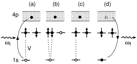
Figure 1: A schematic representation of the two-magnon process in RIXS, corresponding to the first term of Eq. (6); (a) the $1s$ electron is excited to the $4p$ band by absorbing x-ray, (b,c) an exchange process takes place under the influence of the core-hole potential, and (d) the $4p$ electron is recombined with the $1s$-core hole.

The RIXS intensity is simply given by replacing $H_{1s-3d}$ with $H_{1s-3d}^{\rm eff}$ in the NI formula.Nomura and Igarashi (2005) The corresponding diagram in the Keldysh scheme is shown in Fig. 2, where the effective interaction $H_{1s-3d}^{\rm eff}$ is represented by the double line. The incident photon has a momentum $\textbf{q}_{i}$ and an energy $\omega_{i}$, a polarization $\textbf{{e}}^{(\alpha_{i})}$, and the scattered photon has a momentum $\textbf{q}_{f}$ and an energy $\omega_{f}$, a polarization $\textbf{{e}}^{(\alpha_{f})}$. The momentum and the energy transferred from photon are given by $\textbf{q}=\textbf{q}_{i}-\textbf{q}_{f}$ and $\omega=\omega_{i}-\omega_{f}$. They are written simply as $q=(\textbf{q},\omega)$. Similarly, we introduce the notations $q_{i}=(\textbf{q}_{i},\omega_{i})$ and $q_{f}=(\textbf{q}_{f},\omega_{f})$.

The upper triangle represents the product of Green’s functions of the $4p$ electron and the core hole on the outward time leg, which gives a factor, $\exp[i(\epsilon_{4p}^{\eta}({\textbf{p}})-\epsilon_{1s}-i\Gamma_{1s}-\omega_{i})t]$, with $\Gamma_{1s}$ being a lifetime broadening width of the $1s$ core hole. The lower triangle represents the product of Green’s functions on the backward time leg, which gives a factor $\exp[-i(\epsilon_{4p}^{\eta}({\textbf{p}})-\epsilon_{1s}+i\Gamma_{1s}-\omega_{i})(t^{\prime}-u^{\prime})]$. Note that extra time dependent factors, ${\rm e}^{i\omega s}$ on the outward time leg and ${\rm e}^{-i\omega s^{\prime}}$ on the backward time leg, arise from the interaction. Integrating the time factor combined to the above product of Green’s functions, with respect to $s$ and $t$ in the region of $t<s<0$, $-\infty<t<0$, we obtain

$$L_{B}^{\eta}(\omega_{i};\omega) \equiv J_{c}\int_{-\infty}^{0}{\rm d}t\frac{1}{N}\sum_{\textbf{p}}\exp[i(\epsilon_{4p}^{\eta}({\textbf{p}})-\epsilon_{1s}-i\Gamma_{1s}-\omega_{i})t]\int_{t}^{0}{\rm d}s\,{\rm e}^{i\omega s}$$ (9)

$$= -J_{c}\int\frac{\rho^{\eta}_{4p}(\epsilon){\rm d}\epsilon}{(\omega_{i}+\epsilon_{1s}+i\Gamma_{1s}-\epsilon)(\omega_{i}-\omega+\epsilon_{1s}+i\Gamma_{1s}-\epsilon)}.$$

Here the summation over the momentum is replaced by the integration over the energy associated with the $4p$ DOS $\rho_{4p}^{\eta}(\epsilon)$ projected onto the $\eta$ ($=x,y,z$) symmetry. The integration with respect to $s^{\prime}$ and $t^{\prime}$ on the backward time leg gives the term complex conjugate to Eq. (9). The integration with respect to $u^{\prime}$ gives the energy conservation factor, which guarantees that $\omega$ in Eq. (9) is the energy loss, $\omega=\omega_{i}-\omega_{f}$. See Ref. Igarashi et al., 2006 for the detailed derivation of this function. Since the magnon energy is usually an order of $0.5$ eV, which is much smaller than the energy scale of the $4p$ DOS, we can safely put $\omega=0$ in Eq. (9). The bubble with shaded vertexes in Fig. 2 denotes the two-magnon correlation function $Y^{+-}(\text{q},\omega)$,

$$Y^{+-}(\textbf{q},\omega)=\int_{-\infty}^{\infty}\langle M_{\textbf{q}}^{\dagger}(s^{\prime})M_{\textbf{q}}(s)\rangle{\rm e}^{i\omega(s^{\prime}-s)}{\rm d}(s^{\prime}-s),$$ (10)

with

$$M_{\textbf{q}}=\sqrt{\frac{2}{N}}\sum_{n,\delta}\textbf{S}_{n}\cdot\textbf{S}_{n+\delta}{\rm e}^{-i\textbf{q}\cdot\textbf{r}_{n}},$$ (11)

where $\langle\cdots\rangle$ indicates the average over the ground state. Combining all the above factors, we finally obtain the expression of the RIXS intensity as

$$W(q_{i},\alpha_{i};q_{f},\alpha_{f})=\frac{|w|^{4}}{4\omega_{i}\omega_{f}}\frac{N}{2}Y^{+-}(\textbf{q},\omega)\left|\sum_{\eta}e_{\eta}^{(\alpha_{f})}L^{\eta}_{B}(\omega_{i};\omega)e_{\eta}^{(\alpha_{i})}\right|^{2}.$$ (12)

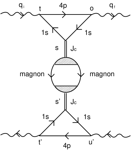
Figure 2: Diagrams for the RIXS intensity in the Keldysh scheme. The double lines represent the effective interaction between the core hole and spins of $3d$ electrons. The solid lines with 4p and 1s denote the Green’s functions of the $4p$ electron and of the $1s$ core hole, respectively. The bubble with shaded vertexes stands for the two-magnon correlation function, which connects the outward time leg on the top half and the backward time leg on the bottom half.

III The 1/S expansion

We carry out systematically the $1/S$-expansion by introducing the Holstein-Primakoff transformation to the spin operators.Holstein and Primakoff (1940) Assuming two sublattices in the AF ground state, we express spin operators by boson operators as

$$S_{i}^{z} = S-a_{i}^{\dagger}a_{i},$$ (13)

$$S_{i}^{+} = (S_{i}^{-})^{\dagger}=\sqrt{2S}f_{i}(S)a_{i},$$ (14)

$$S_{j}^{z} = -S+b_{j}^{\dagger}b_{j},$$ (15)

$$S_{j}^{+} = (S_{j}^{-})^{\dagger}=\sqrt{2S}b_{j}^{\dagger}f_{j}(S),$$ (16)

where $a_{i}$ and $b_{j}$ are boson annihilation operators, and

$$f_{\ell}(S)=\left(1-\frac{n_{\ell}}{2S}\right)^{1/2}\\ =1-\frac{1}{2}\frac{n_{\ell}}{2S}-\frac{1}{8}\left(\frac{n_{\ell}}{2S}\right)^{2}+\cdots,$$ (17)

with $n_{\ell}=a_{i}^{\dagger}a_{i}$ and $b_{j}^{\dagger}b_{j}$. Indices $i$ and $j$ refer to sites on the ”up” and ”down” sublattices, respectively.

III.1 Heisenberg Hamiltonian

First we apply the $1/S$ expansion to the Heisenberg Hamiltonian described by

$$H=J\sum_{<i,j>}\textbf{S}_{i}\cdot\textbf{S}_{j},$$ (18)

where $\langle i,j\rangle$ indicates the sum taken over nearest neighbor pairs. Substituting Eqs. (13)-(16) into Eq. (18) we expand the Hamiltonian in powers of $1/S$ as

$$H=-\frac{1}{2}JS^{2}Nz+H_{0}+H_{1}+\cdots,$$ (19)

where $N$ and $z$ are the number of lattice sites and that of nearest neighbor sites, respectively. The leading term $H_{0}$ is expressed as

$$H_{0}=JS\sum_{<i,j>}(a_{i}^{\dagger}a_{i}+b^{\dagger}_{j}b_{j}+a_{i}b_{j}+a_{i}^{\dagger}b_{j}^{\dagger}).$$ (20)

Rewriting the boson operators in the momentum space as

$$a_{i} = \left(\frac{2}{N}\right)^{1/2}\sum_{\textbf{k}}a_{\textbf{k}}\exp(i\textbf{k}\cdot\textbf{r}_{i}),$$ (21)

$$b_{j} = \left(\frac{2}{N}\right)^{1/2}\sum_{\textbf{k}}b_{\textbf{k}}\exp(i\textbf{k}\cdot\textbf{r}_{j}),$$ (22)

we diagonalize $H_{0}$ by introducing the Bogoliubov transformation,

$$a_{\textbf{k}}^{\dagger}=\ell_{\textbf{k}}\alpha_{\textbf{k}}^{\dagger}+m_{\textbf{k}}\beta_{-\textbf{k}},\quad b_{-\textbf{k}}=m_{\textbf{k}}\alpha_{\textbf{k}}^{\dagger}+\ell_{\textbf{k}}\beta_{-\textbf{k}},$$ (23)

where

$$\ell_{\textbf{k}}=\Bigl{[}\frac{1+\epsilon_{\textbf{k}}}{2\epsilon_{\textbf{k}}}\Bigr{]}^{1/2},\quad m_{\textbf{k}}=-\Bigl{[}\frac{1-\epsilon_{\textbf{k}}}{2\epsilon_{\textbf{k}}}\Bigr{]}^{1/2}\equiv-x_{\textbf{k}}\ell_{\textbf{k}},$$ (24)

with

$$\epsilon_{\textbf{k}}=\sqrt{1-\gamma_{\textbf{k}}^{2}},\quad\gamma_{\textbf{k}}=\frac{1}{z}\sum_{\mbox{\boldmath{$\delta$}}}{\rm e}^{i{\textbf{k}}\cdot\mbox{\boldmath{$\delta$}}}.$$ (25)

Here $\delta$ is the nearest neighbor vectors. Momentum k is defined in the first magnetic Brillouin zone (MBZ).

As shown in Ref. Igarashi, 1992, after the Bogoliubov transformation, the Hamiltonian becomes

$$H_{0} = JSz\sum_{\textbf{k}}(\epsilon_{\textbf{k}}-1)+JSz\sum_{\textbf{k}}\epsilon_{\textbf{k}}(\alpha_{\textbf{k}}^{\dagger}\alpha_{\textbf{k}}+\beta_{\textbf{k}}^{\dagger}\beta_{\textbf{k}}),$$ (26)

$$H_{1} = \frac{JSz}{2S}A\sum_{\textbf{k}}\epsilon_{\textbf{k}}(\alpha_{\textbf{k}}^{\dagger}\alpha_{\textbf{k}}+\beta_{\textbf{k}}^{\dagger}\beta_{\textbf{k}})$$ (27)

$$+ \frac{-JSz}{2SN}\sum_{1234}\delta_{\textbf{G}}(1+2-3-4)\ell_{1}\ell_{2}\ell_{3}\ell_{4}$$

$$\times \biggl{[}\alpha_{1}^{\dagger}\alpha_{2}^{\dagger}\alpha_{3}\alpha_{4}B_{1234}^{(1)}+\beta_{-3}^{\dagger}\beta_{-4}^{\dagger}\beta_{-1}\beta_{-2}B_{1234}^{(2)}+4\alpha_{1}^{\dagger}\beta_{-4}^{\dagger}\beta_{-2}\alpha_{3}B_{1234}^{(3)}$$

$$+ \bigl{(}2\alpha_{1}^{\dagger}\beta_{-2}\alpha_{3}\alpha_{4}B_{1234}^{(4)}+2\beta_{-4}^{\dagger}\beta_{-1}\beta_{-2}\alpha_{3}B_{1234}^{(5)}+\alpha_{1}^{\dagger}\alpha_{2}^{\dagger}\beta_{-3}^{\dagger}\beta_{-4}^{\dagger}B_{1234}^{(6)}+{\rm H.c.}\bigr{)}\biggr{]},$$

with

$$A=\frac{2}{N}\sum_{\textbf{k}}(1-\epsilon_{\textbf{k}}).$$ (28)

The first term in Eq. (27) arises from setting the products of four boson operators into normal product forms with respect to magnon operators, known as the Oguchi correction.Oguchi (1960) For the square lattice, $A=0.1579$. The second term represents the scattering of magnons. Momenta $\textbf{k}_{1}$, $\textbf{k}_{2}$, $\textbf{k}_{3}$, $\cdots$ are abbreviated as $1,2,3,\cdots$. The Kronecker delta $\delta_{\textbf{G}}(1+2-3-4)$ indicates the conservation of momenta within a reciprocal lattice vector G. Explicit expressions for $B^{(i)}$’s in a symmetric parameterization are given by Eqs. (2.16)-(2.20) in Ref. Igarashi, 1992. Here we only write down the explicit expression of $B^{(3)}_{1234}$, which will become necessary in the next section,

$$B^{(3)}_{1234} = \gamma_{2-4}+\gamma_{1-3}x_{1}x_{2}x_{3}x_{4}+\gamma_{1-4}x_{1}x_{2}+\gamma_{2-3}x_{3}x_{4}$$ (29)

$$- \frac{1}{2}(\gamma_{2}x_{4}+\gamma_{1}x_{1}x_{2}x_{4}+\gamma_{2-3-4}x_{3}+\gamma_{1-3-4}x_{1}x_{2}x_{3}+\gamma_{4}x_{2}$$

$$+ \gamma_{3}x_{2}x_{3}x_{4}+\gamma_{4-2-1}x_{1}+\gamma_{3-2-1}x_{1}x_{3}x_{4}).$$

III.2 Two-magnon operator

Inserting Eqs. (13) $\sim$ (16) into Eq. (11), we expand $M_{\textbf{q}}$ in terms of boson operators as

$$M_{\textbf{q}} = S\sqrt{\frac{2}{N}}\sum_{\delta}\biggl{[}\sum_{i\in A}(a_{i}^{\dagger}a_{i}+b_{i+\delta}^{\dagger}b_{i+\delta}+a_{i}b_{i+\delta}+a_{i}^{\dagger}b_{i+\delta}^{\dagger}){\rm e}^{i\textbf{q}\cdot\textbf{{r}}_{i}}$$ (30)

$$+\sum_{j\in B}(b_{j}^{\dagger}b_{j}+a_{j+\delta}^{\dagger}a_{j+\delta}+b_{j}a_{j+\delta}+b_{j}^{\dagger}a_{j+\delta}^{\dagger}){\rm e}^{i\textbf{q}\cdot\textbf{{r}}_{j}}\biggr{]}.$$

Note that the momentum transfer q is defined in the first BZ, which is the double of the first MBZ. When q is outside the first MBZ, it can be brought back to the first MBZ by a reciprocal vector $\textbf{G}_{0}$, that is, $\textbf{q}=\textbf{q}_{0}+\textbf{G}_{0}$ with $\textbf{q}_{0}$ being inside the first MBZ. In this situation, ${\rm e}^{i\textbf{q}\cdot\textbf{{r}}_{j}}=-{\rm e}^{i\textbf{q}_{0}\cdot\textbf{{r}}_{j}}$ in the second term of Eq. (30). Noting this fact and substituting Eq. (23) into Eq. (30), we obtain the expression of $M_{\textbf{q}}$ as

$$M_{\textbf{q}}=\sqrt{\frac{2}{N}}\sum_{\textbf{k}}N(\textbf{q},\textbf{k})\alpha_{[\textbf{q}_{0}+\textbf{k}]}^{\dagger}\beta_{-\textbf{k}}^{\dagger}+{\textrm{H}.c.}+\cdots,$$ (31)

with

$$N(\textbf{q},\textbf{k}) = Sz\bigl{\{}(1\pm\gamma_{\textbf{q}_{0}})\ell_{[\textbf{q}_{0}+\textbf{k}]}m_{\textbf{k}}+\textrm{sgn}(\gamma_{\textbf{G}})(\pm 1+\gamma_{\textbf{q}_{0}})m_{[\textbf{q}_{0}+\textbf{k}]}\ell_{\textbf{k}}$$ (32)

$$+ [\gamma_{[\textbf{q}_{0}+\textbf{k}]}\pm\textrm{sgn}(\gamma_{\textbf{G}})\gamma_{\textbf{k}}]m_{[\textbf{q}_{0}+\textbf{k}]}m_{\textbf{k}}+[\gamma_{\textbf{k}}\pm\textrm{sgn}(\gamma_{\textbf{G}})\gamma_{[\textbf{q}_{0}+\textbf{k}]}]\ell_{[\textbf{q}_{0}+\textbf{k}]}\ell_{\textbf{k}}\bigr{\}}.$$

Sign $\pm$ corresponds to the case that q is inside or outside the first MBZ. Symbol $[\textbf{q}_{0}+\textbf{k}]$ stands for the $\textbf{q}_{0}+\textbf{k}$ reduced in the first MBZ by a reciprocal lattice vector G, that is, $[\textbf{q}_{0}+\textbf{k}]=\textbf{q}_{0}+\textbf{k}-\textbf{G}$, and $\textrm{sgn}(\gamma_{\textbf{G}})$ denotes the sign of $\gamma_{\textbf{G}}$. This result will be used to calculate $Y^{+-}(\text{q},\omega)$ in the next section. Note that $N(\textbf{q},\textbf{k})=0$ for $\textbf{q}=0$ and $\textbf{q}=(\pi,\pi)$ in the square lattice, indicating that no RIXS signal would be generated.

III.3 Two-magnon correlation function

Defining the two-magnon Green’s function as

$$F(\textbf{q}_{0},\omega;\textbf{k},\textbf{k}^{\prime})=-i\int\textrm{e}^{i\omega t}{\rm d}t\langle T[\beta_{-\textbf{k}}(t)\alpha_{[\textbf{q}_{0}+\textbf{k}]}(t)\alpha_{[\textbf{q}_{0}+\textbf{k}^{\prime}]}^{\dagger}\beta_{-\textbf{k}^{\prime}}^{\dagger}]\rangle,$$ (33)

we rewrite the two-magnon correlation function $Y^{+-}(\text{q},\omega)$ as

$$Y^{+-}(\textbf{q},\omega)=\frac{2}{N}\sum_{\textbf{k}}\sum_{\textbf{k}^{\prime}}N(\textbf{q},\textbf{k})N(\textbf{q},\textbf{k}^{\prime})(-2){\rm Im}F(\textbf{q}_{0},\omega;\textbf{k},\textbf{k}^{\prime}).$$ (34)

Here T is the time-ordering operator. The two-magnon Green’s function is expanded in terms of the one-magnon Green functions,

$$G_{\alpha\alpha}({\textbf{k}},t) = -i\langle T[\alpha_{\textbf{k}}(t)\alpha_{\textbf{k}}^{\dagger}(0)]\rangle,$$ (35)

$$G_{\beta\beta}(\textbf{k},t) = -i\langle T[\beta_{{\textbf{k}}}(t)\beta_{\textbf{k}}^{\dagger}(0)]\rangle.$$ (36)

The unperturbed ones corresponding to $H_{0}$ are given by

$$G_{\alpha\alpha}^{(0)}(\textbf{k},\omega)=G_{\beta\beta}^{(0)}(\textbf{k},\omega)=[\omega-\epsilon_{\textbf{k}}+i\eta]^{-1},\quad\eta\to 0^{+},$$ (37)

in the energy unit of $JSz$. Hereafter we use this energy unit.

In the lowest order, the two-magnon Green’s function is simply given by

$$F(\textbf{q}_{0},\omega;\textbf{k},\textbf{k}^{\prime})=F_{0}(\textbf{q}_{0},\omega;\textbf{k})\delta_{\textbf{k},\textbf{k}^{\prime}},$$ (38)

with

$$F_{0}(\textbf{q}_{0},\omega;\textbf{k}) = i\int G^{(0)}_{\alpha\alpha}([\textbf{q}_{0}+\textbf{k}],\omega+k_{0})G^{(0)}_{\beta\beta}(-\textbf{k},-k_{0})\frac{dk_{0}}{2\pi}$$ (39)

$$= \frac{1}{\omega-\epsilon_{[\textbf{q}_{0}+\textbf{k}]}-\epsilon_{\textbf{k}}+i\eta}.$$

Inserting this relation into Eq. (34), we obtain the correlation function in the lowest order as

$$Y^{(0)+-}(\textbf{q},\omega)=2\pi\frac{2}{N}\sum_{\textbf{k}}N(\textbf{q},\textbf{k})^{2}\delta(\omega-\epsilon_{[\textbf{q}_{0}+\textbf{k}]}-\epsilon_{\textbf{k}}).$$ (40)

In the first order in $1/S$, the magnon energy $\epsilon_{\textbf{k}}$ is changed into $(1+\frac{A}{2S})\epsilon_{\textbf{k}}$ due to the Oguchi correction. Therefore, $F_{0}(\textbf{q},\omega;\textbf{k})$ is modified by replacing $\epsilon_{[\textbf{q}_{0}+\textbf{k}]}$ and $\epsilon_{[\textbf{k}]}$ in Eq. (39) with $(1+\frac{A}{2S})\epsilon_{[\textbf{q}_{0}+\textbf{k}]}$ and $(1+\frac{A}{2S})\epsilon_{\textbf{k}}$, respectively. Let $\bar{F}_{0}(\textbf{q},\omega;\textbf{k})$ be the function after this modification. Within the same order, we have to take account of the magnon-magnon interaction. Only the terms of a factor $B^{(3)}_{1234}$ in Eq. (27) is relevant to the present calculation. Consider the ladder approximation shown in Fig. 3 for the two-magnon Green’s function. Regarding the dependence on k and $\textbf{k}^{\prime}$ in $F(\textbf{q}_{0},\omega;\textbf{k},\textbf{k}^{\prime})$ as a matrix $\hat{F}(\textbf{q}_{0},\omega)$ with $\frac{N}{2}\times\frac{N}{2}$ dimensions, we notice that the sum of the ladder diagrams is equivalent to the expression,

$$\left[\hat{F}(\textbf{q}_{0},\omega)^{-1}\right]_{\textbf{k},\textbf{k}^{\prime}}=\bar{F}_{0}(\textbf{q}_{0},\omega;\textbf{k})^{-1}\delta_{\textbf{k},\textbf{k}^{\prime}}+\frac{4}{2SN}\ell_{[\textbf{q}_{0}+\textbf{k}^{\prime}]}\ell_{\textbf{k}}\ell_{[\textbf{q}_{0}+\textbf{k}]}\ell_{\textbf{k}^{\prime}}B^{(3)}_{[\textbf{q}_{0}+\textbf{k}^{\prime}],{\textbf{k},[\textbf{q}_{0}+\textbf{k}],\textbf{k}^{\prime}}}.$$ (41)

This is nothing but the eigenvalue equation for two-magnon excitations, indicating that the ladder approximation together with the Oguchi correction to the single-magnon energy constitute the first-order correction in the $1/S$ expansion.

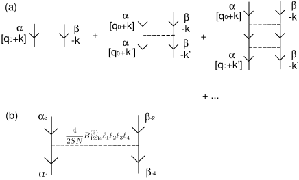
Figure 3: (a) Ladder diagrams for $F(\textbf{q}_{0},\omega;\textbf{k},\textbf{k}^{\prime})$. Solid lines represent the single-magnon Green’s function with the magnon energy including the Oguchi correction. (b) Magnon-magnon interaction in units of $JSz$.

Equation (41) is not useful for the actual calculation of the two-magnon Green’s function, because the matrix with $\frac{N}{2}\times\frac{N}{2}$ dimensions has to be inverted in order to get $\hat{F}(\textbf{q}_{0},\omega)$. We sum up exactly the ladder diagrams, transforming the interaction into a separable form with several channels,

$$-\frac{4}{2SN}\ell_{1}\ell_{2}\ell_{3}\ell_{4}B_{1234}^{(3)}=\sum_{m,n=1}^{N_{c}}v_{m}(2,3)\Gamma_{mn}v_{n}(4,1).$$ (42)

Here $N_{c}$ is the channel number. The indices $2$ and $3$ specify the incoming magnons while $1$ and $4$ specify the outgoing magnons (Fig. 3(b)). Explicit forms of $v_{n}(\textbf{k},\textbf{k}^{\prime})$ and $\Gamma_{mn}$ are given for the square lattice in the next section. Thereby we obtain the T-matrix $\Pi$,

$$\Pi(\textbf{q}_{0},\omega:\textbf{k},\textbf{k}^{\prime})=\frac{2}{N}\sum_{m,n}v_{m}(\textbf{k},[\textbf{q}_{0}+\textbf{k}])\Gamma^{\rm eff}_{mn}(\textbf{q}_{0},\omega)v_{n}(\textbf{k}^{\prime},[\textbf{q}_{0}+\textbf{k}^{\prime}]),$$ (43)

where

$$\Gamma^{\rm eff}_{mn}(\textbf{q}_{0},\omega)=\left[[\textbf{I}-\hat{\Gamma}\hat{R}(\textbf{q}_{0},\omega)]^{-1}\hat{\Gamma}\right]_{mn},$$ (44)

with

$$[{\hat{R}}(\textbf{q}_{0},\omega)]_{mn}=\frac{2}{N}\sum_{\textbf{k}}v_{m}(\textbf{k},[\textbf{q}_{0}+\textbf{k}])\bar{F}_{0}(\textbf{q}_{0},\omega;\textbf{k})v_{n}(\textbf{k},[\textbf{q}_{0}+\textbf{k}]).$$ (45)

In Eq. (44), the unit matrix $\hat{\textbf{1}}$ and $\hat{R}(\textbf{q}_{0},\omega)$ are in the $N_{c}\times N_{c}$ dimensions. We calculate the two-magnon Green’s function from the T-matrix,

$$F(\textbf{q}_{0},\omega;\textbf{k},\textbf{k}^{\prime})=\bar{F}_{0}(\textbf{q}_{0},\omega;\textbf{k})\left[\delta_{\textbf{k},\textbf{k}^{\prime}}+\Pi(\textbf{q}_{0},\omega:\textbf{k},\textbf{k}^{\prime})\bar{F}_{0}(\textbf{q}_{0},\omega;\textbf{k}^{\prime})\right].$$ (46)

Inserting this equation into Eq. (34), we obtain $Y^{+-}(\textbf{q},\omega)$, which gives the RIXS intensity as a function of momentum and energy transferred from photon.

IV Calculated Results

We apply the formulas in the preceding sections to La₂CuO₄, which seems to be a typical two-dimensional Heisenberg antiferromagnet. The RIXS intensity in the two-magnon region relative to that in the charge excitation region is roughly estimated as $(J_{c}/V)^{2}$. For La₂CuO₄, we have $(J_{c}/V)^{2}<0.01$, because $J_{c}\sim 0.2-0.5$ eV and $V\sim 5-10$ eV.

IV.1 Incident-photon-energy dependence

We carry out the band calculation for La₂CuO₄ within the LDA. Figure 4(a) shows the $4p$ DOS projected onto the $p_{z}$ and $p_{x}$ ($p_{y}$) symmetries, which may correspond to the absorption coefficients for the photon polarization along the $c$ axis and in the $ab$ plane, respectively.

Using the same DOS, we calculate the factor determining the incident-photon-energy dependence, $|\sum_{\eta}e_{\eta}^{(\alpha)}L^{\eta}_{B}(\omega_{i};\omega=0)e_{\eta}^{(\alpha)}|^{2}$, for the incident and scattered photons having the same polarization. Figure 4(b) shows the calculated results for the polarization along the $c$-axis and in the $ab$-plane. A strong resonant enhancement is predicted as a function of incident photon energy. The enhancement for polarization along the $c$ axis is much stronger than that in the $ab$ plane. This is quite different from light scattering where the polarization of light is restricted in the $ab$ plane (see Appendix).Parkinson (1969)

Figure 4: (a) The $4p$ DOS projected onto the $p_{z}$ and $p_{x}$ ($p_{y}$) symmetries, calculated by the LDA in La$2$CuO₄. The origin of the energy is the bottom of the $4p$ band. (b) The RIXS intensity proportional to $|\sum_{\eta}e_{\eta}^{(\alpha)}L^{\eta}_{B}(\omega_{i};\omega=0)e_{\eta}^{(\alpha)}|^{2}$, with ${\rm e}^{(\alpha)}$ along the $c$ axis and in the $ab$ plane. The origin of the energy corresponds to the photon energy of exciting the $1s$ core electron into the bottom of the $4p$ band.

IV.2 Momentum dependence as a function of energy loss

We consider the Heisenberg model on a square lattice. We put $\gamma_{\textbf{k}}=(\cos k_{x}+\cos k_{y})/2$ with $k_{x}$, $k_{y}$ in units of 1/(lattice constant). For the magnon-magnon interaction, we have the channel number $N_{c}=13$, and $\hat{\Gamma}$ is given by

$$\hat{\Gamma}\equiv-\frac{4}{2SN}\left(\begin{array}[]{ccccccccccccc}0&-1&-1&2&2&-1&-1&0&0&0&0&0&0\\ -1&2&0&-1&0&0&0&0&0&0&0&0&0\\ -1&0&2&0&-1&0&0&0&0&0&0&0&0\\ 2&-1&0&0&0&-1&0&0&0&0&0&0&0\\ 2&0&-1&0&0&0&-1&0&0&0&0&0&0\\ -1&0&0&-1&0&2&0&0&0&0&0&0&0\\ -1&0&0&0&-1&0&2&0&0&0&0&0&0\\ 0&0&0&0&0&0&0&2&0&-1&0&0&0\\ 0&0&0&0&0&0&0&0&2&0&-1&0&0\\ 0&0&0&0&0&0&0&-1&0&0&0&1&0\\ 0&0&0&0&0&0&0&0&-1&0&0&0&1\\ 0&0&0&0&0&0&0&0&0&1&0&2&0\\ 0&0&0&0&0&0&0&0&0&0&1&0&2\\ \end{array}\right).$$ (47)

The $v_{n}(\textbf{k},\textbf{k}^{\prime})$’s are defined in Table 1. In the actual calculation, we divide the first MBZ into $512\times 512$ meshes, and carry out the sum over k in Eq. (45) to evaluate $\hat{R}(\textbf{q}_{0},\omega)$.

Table 1: Definition of the coefficients $v_{n}(\textbf{k},\textbf{k}^{\prime})$

$n$	$v_{n}(\textbf{k},\textbf{k}^{\prime})$
1	$\frac{1}{2}\ell_{\textbf{k}}\ell_{\textbf{k}^{\prime}}x_{\textbf{k}}$
2	$\frac{1}{2}\ell_{\textbf{k}}\ell_{\textbf{k}^{\prime}}\cos k_{x}$
3	$\frac{1}{2}\ell_{\textbf{k}}\ell_{\textbf{k}^{\prime}}\cos k_{y}$
4	$\frac{1}{2}\ell_{\textbf{k}}\ell_{\textbf{k}^{\prime}}x_{\textbf{k}^{\prime}}\cos(k_{x}-k_{x}^{\prime})$
5	$\frac{1}{2}\ell_{\textbf{k}}\ell_{\textbf{k}^{\prime}}x_{\textbf{k}^{\prime}}\cos(k_{y}-k_{y}^{\prime})$
6	$\frac{1}{2}\ell_{\textbf{k}}\ell_{\textbf{k}^{\prime}}x_{\textbf{k}}x_{\textbf{k}^{\prime}}\cos k_{x}^{\prime}$
7	$\frac{1}{2}\ell_{\textbf{k}}\ell_{\textbf{k}^{\prime}}x_{\textbf{k}}x_{\textbf{k}^{\prime}}\cos k_{y}^{\prime}$
8	$\frac{1}{2}\ell_{\textbf{k}}\ell_{\textbf{k}^{\prime}}\sin k_{x}$
9	$\frac{1}{2}\ell_{\textbf{k}}\ell_{\textbf{k}^{\prime}}\sin k_{y}$
10	$\frac{1}{2}\ell_{\textbf{k}}\ell_{\textbf{k}^{\prime}}x_{\textbf{k}^{\prime}}\sin(k_{x}-k_{x}^{\prime})$
11	$\frac{1}{2}\ell_{\textbf{k}}\ell_{\textbf{k}^{\prime}}x_{\textbf{k}^{\prime}}\sin(k_{y}-k_{y}^{\prime})$
12	$\frac{1}{2}\ell_{\textbf{k}}\ell_{\textbf{k}^{\prime}}x_{\textbf{k}}x_{\textbf{k}^{\prime}}\sin k_{x}^{\prime}$
13	$\frac{1}{2}\ell_{\textbf{k}}\ell_{\textbf{k}^{\prime}}x_{\textbf{k}}x_{\textbf{k}^{\prime}}\sin k_{y}^{\prime}$

Figure 5 shows the calculated RIXS intensity $Y^{+-}(\textbf{q},\omega)$ scaled by $(Sz)^{2}$ as a function of energy loss $\omega$ for several typical values of q. The lowest order value, $Y^{(0)+-}(\textbf{q},\omega)/(Sz)^{2}$, is independent of $S$, corresponding to $S=\infty$. The effect of the magnon-magnon interaction becomes weaker with increasing $S$, and the spectra approach to the lowest-order values. As already pointed out, no RIXS intensity comes out at the $\Gamma$ point and at $\textbf{q}=(\pi,\pi)$. When q is close to the $\Gamma$ point (panel (a)), a sharp peak is found for $\omega<JSz$, which is slightly modified in the presence of the magnon-magnon interaction. When q is at the boundary of the first MBZ (panels (b) and (c)), a sharp peak found in the lowest order approximation is smeared out to be a broad peak due to the magnon-magnon interaction. The center of the shape remains nearly the same after taking account of the interaction. In contrast to these cases, when q is outside the first MBZ (panel (d)), a sharp peak found in the lowest order approximation is changed into a broad peak with its center considerably shifted to the lower energy region due to the magnon-magnon interaction.

Figure 5: The RIXS intensity $Y^{+-}(\textbf{q},\omega)$ scaled by $(Sz)^{2}$ as a function of $\omega/JSz$ for typical values of q. The bold and thin solid lines stand for $Y^{+-}(\textbf{q},\omega)/(Sz)^{2}$ with $S=\frac{1}{2}$ and $1$, respectively. The broken lines represent $Y^{(0)+-}(\textbf{q},\omega)/(Sz)^{2}$, which correspond to $S\to\infty$.

Figure 6 shows the RIXS spectra as a function of energy loss with changing momenta along several symmetry lines ($S=1/2$). Along the zone boundary of the first MBZ (panel (b)), the spectra have large widths around $\omega=3J$. The spectra obtained here seem to be different from the results of van den Brink,van den Brink who made the moment analysis. We find no long-lived virtual bound state of two magnons, which has been predicted on the phonon assisted light absorption spectra.Lorenzana and Sawatzky (1995) Note that the matrix elements of creating two magnons in RIXS are different from those in light scattering.Donkov and Chubukov Since the spectral shape depends strongly on the matrix elements, the direct comparison of the two spectra may be less useful. The present formalism recovers the results of light scattering (at $\textbf{q}=0$) by Canali and Girvin,Canali and Girvin (1992) as shown in Appendix.

The exchange coupling constant $J$ in La₂CuO₄ is estimated as $J=135$ meV by comparing the spin-wave velocity calculated in the first order of $1/S$ with the experiment.Aeppli et al. (1989) Therefore, the broad peaks are located around $\omega=400$ meV for q at the boundary of the first MBZ, Unfortunately, no experimental data are available on such a low energy region in La₂CuO₄.

Figure 6: The RIXS intensity $Y^{+-}(\textbf{q},\omega)/(Sz)^{2}$ along the symmetry lines for q within the first order of $1/S$ ($S=1/2$).

V Concluding Remarks

We have formulated the two-magnon spectra of RIXS in antiferromagnets by developing the formalism of Nomura and Igarashi. The $1s$ core hole potential causes a change in the exchange coupling between $3d$ electrons, resulting in the two-magnon excitation. This is analogous to the conventional RIXS process that the charge excitation is created due to the screening of the core hole potential. The intensity of two-magnon RIXS is estimated to be lass than 0.01 of the intensity coming from the charge excitation.

In the present formalism, the factor describing the incident-photon-energy dependence is separated from the factor describing the dependence on the momentum and the energy transferred from photon. We have calculated the former factor using the $4p$ DOS for La₂CuO₄ within the LDA. We have predicted a strong enhancement of the intensity at the $K$ edge for the polarization along the $c$ axis. The latter factor is given by the two-magnon correlation function. We have calculated the correlation function up to the first order of $1/S$ in the square lattice, systematically applying the $1/S$ expansion. We have exactly summed up the ladder diagrams by transforming the magnon-magnon interaction into a separable form with 13 channels. The spectral shape as a function of energy loss is strongly modified by the magnon-magnon interaction. On the boundary of the first MBZ, for example, the sharp peaks found in the lowest-order approximation have considerably been broadened. We hope the spectra obtained in this paper would be compared with the experimental data in future.

No AF-long-range order could exist at finite temperatures in purely two-dimensional Heisenberg models. In the absence of the AF order, however, it is known from the non-linear $\sigma$ model analysisChakravarty et al. (1989) that the spin-spin correlation length is rather long up to $T\sim J/k_{B}$ The spin-wave-like excitations could exist in such a situation. Tyč et al. (1989); Makivić and -Q. Ding (1991); Nagao and Igarashi (1998) Therefore, the present analysis of the RIXS spectra at zero temperature may have relevance to the spectra at finite temperatures. The analysis of temperature effects is left in future study.

Appendix A Two-magnon light scattering

We summarize the two-magnon excitation of light scattering to compare the result by the present formalism with previous studies in two dimensions.

Since the wavelength of light is much longer than the lattice spacing, the intensity is independent of the directions of the incident and scattered lights. The interaction of light with spins is described byParkinson (1969)

$$H_{R}=\sum_{j\mbox{\boldmath{$\delta$}}}\left[A(\textbf{e}_{i}\cdot\mbox{\boldmath{$\delta$}})(\textbf{e}_{f}\cdot\mbox{\boldmath{$\delta$}})+B(\textbf{e}_{i}\cdot\textbf{e}_{f})+Ce_{i}^{z}e_{f}^{z}\right](\textbf{S}_{j}\cdot\textbf{S}_{j+\mbox{\boldmath{$\delta$}}}),$$ (48)

where $\delta$ is a unit vector in the direction joining the nearest neighbor pairs and $A,B$, and $C$ are real constants. The terms with $B$ and $C$ cannot cause scattering, since they are proportional to $\sum_{j\mbox{\boldmath{$\delta$}}}\textbf{S}_{j}\cdot\textbf{S}_{j+\mbox{\boldmath{$\delta$}}}$ and commute with the magnetic Hamiltonian. For the polarization picking up the $A_{1g}$ mode, $\textbf{e}_{i}=(\hat{\textbf{x}}+\hat{\textbf{y}})/\sqrt{2}$, $\textbf{e}_{f}=(\hat{\textbf{x}}+\hat{\textbf{y}})/\sqrt{2}$, no intensity comes out by the same reason ($\hat{\textbf{x}}$ and $\hat{\textbf{y}}$ are unit vectors pointing to the $x$ and $y$ axes). For the polarization picking up the $B_{1g}$ mode, $\textbf{e}_{i}=(\hat{\textbf{x}}+\hat{\textbf{y}})/\sqrt{2}$, $\textbf{e}_{f}=(\hat{\textbf{x}}-\hat{\textbf{y}})/\sqrt{2}$, we have

$$H_{R}=A\sum_{j}\left(\textbf{S}_{j}\cdot\textbf{S}_{j+\hat{\textbf{x}}}-\textbf{S}_{j}\cdot\textbf{S}_{j+\hat{\textbf{y}}}\right).$$ (49)

Expanding this in terms of magnon operators, we obtain

$$H_{R}=ASz\sum_{\textbf{k}}\frac{\gamma^{d}_{\textbf{k}}}{\epsilon_{\textbf{k}}}\left(\alpha_{\textbf{k}}^{\dagger}\beta_{-\textbf{k}}+{\rm H.c.}+\cdots\right),$$ (50)

where $\gamma^{d}_{\textbf{k}}=(\cos k_{x}-\cos k_{y})/2$. The scattering intensity $I(\omega)$ from this interaction is given by

$$I(\omega)\propto(ASz)^{2}\sum_{\textbf{k},\textbf{k}^{\prime}}\left(\frac{\gamma^{d}_{\textbf{k}}\gamma^{d}_{\textbf{k}^{\prime}}}{\epsilon_{\textbf{k}}\epsilon_{\textbf{k}^{\prime}}}\right)(-2){\rm Im}F(\textbf{q}=0,\omega;\textbf{k},\textbf{k}^{\prime}).$$ (51)

We calculate $F(\textbf{q}=0,\omega;\textbf{k},\textbf{k}^{\prime})$ by summing up the ladder diagrams including the Oguchi correction within the present formalism. We obtain the spectrum identical to that of Canali and Girvin, which is formed by a single peak at $\omega=3.38$ for $S=1/2$.Canali and Girvin (1992)

References

• -C. Kao et al. (1996) C. -C. Kao, W. A. L. Caliebe, J. B. Hastings, and J. -M. Gillet, Phys. Rev. B 54, 16361 (1996).
• Hill et al. (1998) J. P. Hill, C. -C. Kao, W. A. L. Calieve, M. Matsubara, A. Kotani, J. L. Peng, and R. L. Greene, Phys. Rev. Lett. 80, 4967 (1998).
• Hasan et al. (2000) M. Z. Hasan, E. D. Isaacs, Z. -X. Shen, L. L. Miller, K. Tsutsui, T. Tohyama, and S. Maekawa, Science 288, 1811 (2000).
• Kim et al. (2002) Y. J. Kim, J. P. Hill, C. A. Burns, S. Wakimoto, R. J. Birgeneau, D. Casa, T. Gog, and C. T. Venkataraman, Phys. Rev. Lett. 89, 177003 (2002).
• Inami et al. (2003) T. Inami, T. Fukuda, J. Mizuki, S. Ishikawa, H. Kondo, H. Nakao, T. Matsumura, K. Hirota, Y. Murakami, S. Maekawa, et al., Phys. Rev. B 67, 45108 (2003).
• Kim et al. (2004) Y. J. Kim, J. P. Hill, H. Benthien, F. H. L. Essler, E. Jeckelmann, H. S. Choi, T. W. Noh, N. Motoyama, K. M. Kojima, S. Uchida, et al., Phys. Rev. Lett. 92, 137402 (2004).
• Suga et al. (2005) S. Suga, S. Imada, A. Higashiya, A. Shigemoto, S. Kasai, M. Sing, H. Fujiwara, A. Sekiyama, A. Yamasaki, C. Kim, et al., Phys. Rev. B 72, 081101(R) (2005).
• Nomura and Igarashi (2004) T. Nomura and J. Igarashi, J. Phys. Soc. Jpn. 73, 1677 (2004).
• Nomura and Igarashi (2005) T. Nomura and J. Igarashi, Phys. Rev. B 71, 035110 (2005).
• Igarashi et al. (2006) J. Igarashi, T. Nomura, and M. Takahashi, Phys. Rev. B 74, 245122 (2006).
• Nozières and Abrahams (1974) P. Nozières and E. Abrahams, Phys. Rev. B 10, 3099 (1974).
• (12) M. Takahashi, J. Igarashi, and T. Nomura, eprint cond-mat/0611656.
• Tsutsui et al. (1999) K. Tsutsui, T. Tohyama, and S. Maekawa, Phys. Rev. Lett. 83, 3705 (1999).
• Okada and Kotani (2006) K. Okada and A. Kotani, J. Phys. Soc. Jpn. 75, 044702 (2006).
• (15) J. P. Hill, talk at the international workshop on X-Ray Scattering and Electronic Stuructures, at SPring-8 Hyogo, Japan, on June 5-7, 2006.
• (16) J. van den Brink, eprint cond-mat/0510140.
• Anderson (1952) P. W. Anderson, Phys. Rev. 86, 694 (1952).
• Kubo (1952) R. Kubo, Phys. Rev. 87, 568 (1952).
• Oguchi (1960) T. Oguchi, Phys. Rev. 117, 117 (1960).
• Harris et al. (1971) A. B. Harris, D. Kumar, B. I. Halperin, and P. C. Hohenberg, Phys. Rev. B 3, 961 (1971).
• Igarashi (1992) J. Igarashi, Phys. Rev. B 46, 10763 (1992).
• Igarashi (1993) J. Igarashi, J. Phys. Soc. Jpn. 62, 4449 (1993).
• Canali et al. (1992) C. M. Canali, S. M. Girvin, and M. Wallin, Phys. Rev. B 45, 10131 (1992).
• Hamer et al. (1992) C. J. Hamer, W. Zheng, and P. Arndt, Phys. Rev. B 46, 6276 (1992).
• Igarashi and Nagao (2005) J. Igarashi and T. Nagao, Phys. Rev. B 72, 014403 (2005).
• Fleury and Loudon (1968) P. A. Fleury and R. Loudon, Phys. Rev. 166, 514 (1968).
• Elliott and Thorpe (1969) R. J. Elliott and M. F. Thorpe, J. Phys. C 2, 1630 (1969).
• Parkinson (1969) J. B. Parkinson, J. Phys. C 2, 2012 (1969).
• Singh et al. (1989) R. R. P. Singh, P. A. Fleury, K. B. Lyons, and P. E. Sulewski, Phys. Rev. Lett. 62, 2736 (1989).
• Canali and Girvin (1992) C. M. Canali and S. M. Girvin, Phys. Rev. B 45, 7127 (1992).
• Sandvik et al. (1998) A. W. Sandvik, S. Capponi, D. Poilblanc, and E. Dagotto, Phys. Rev. B 57, 8478 (1998).
• Lorenzana and Sawatzky (1995) J. Lorenzana and G. A. Sawatzky, Phys. Rev. B 52, 9576 (1995).
• (33) A. Donkov and A. V. Chubukov, eprint cond-mat/0609002.
• Holstein and Primakoff (1940) T. Holstein and H. Primakoff, Phys. Rev. 58, 1098 (1940).
• Aeppli et al. (1989) G. Aeppli, S. M. Hayden, H. A. Mook, Z. Fisk, S. -W. Cheong, D. Rytz, J. P. Remeika, G. P. Espinosa, and A. S. Cooper, Phys. Rev. Lett. 62, 2052 (1989).
• Chakravarty et al. (1989) S. Chakravarty, B. I. Halperin, and D. R. Nelson, Phys. Rev. B 39, 2344 (1989).
• Tyč et al. (1989) S. Tyč, B. I. Halperin, and S. Chakravarty, Phys. Rev. Lett. 62, 835 (1989).
• Makivić and -Q. Ding (1991) M. S. Makivić and H. -Q. Ding, Phys. Rev. B 43, 3562 (1991).
• Nagao and Igarashi (1998) T. Nagao and J. Igarashi, J. Phys. Soc. Jpn. 67, 1029 (1998).