Large Deviations of the Maximum Eigenvalue in Wishart Random Matrices

Abstract

We compute analytically the probability of large fluctuations to the left of the mean of the largest eigenvalue in the Wishart (Laguerre) ensemble of positive definite random matrices. We show that the probability that all the eigenvalues of a ($N\times N$) Wishart matrix $W=X^{T}X$ (where $X$ is a rectangular $M\times N$ matrix with independent Gaussian entries) are smaller than the mean value $\langle\lambda\rangle=N/c$ decreases for large $N$ as $\sim\exp\left[-\frac{\beta}{2}N^{2}\Phi_{-}\left(\frac{2}{\sqrt{c}}+1;c\right)\right]$, where $\beta=1,2$ corresponds respectively to real and complex Wishart matrices, $c=N/M\leq 1$ and $\Phi_{-}(x;c)$ is a rate (sometimes also called large deviation) function that we compute explicitly. The result for the Anti-Wishart case ($M<N$) simply follows by exchanging $M$ and $N$. We also analytically determine the average spectral density of an ensemble of Wishart matrices whose eigenvalues are constrained to be smaller than a fixed barrier. Numerical simulations are in excellent agreement with the analytical predictions.

I Introduction

Consider a rectangular $(M\times N)$ matrix $X$ whose elements $X_{ij}$ represent some data. The $N$ entries of each of the $M$ rows constitute the components of an $N$-dimensional vector $\vec{X}_{i}$ (with $i=1,2,\ldots,M$). The vector $\vec{X}_{i}$ (the $i$-th row of the array) represents the $i$-th sample of the data and the matrix element $X_{ij}$ represents the $j$-th component of the vector ${\vec{X}_{i}}$. For example, suppose we are considering a population of $M$ students in a class, and for each student we have the data of their heights, their marks in an examination, their weights etc. forming a vector of $N$ elements (or traits) for each of the $M$ students. Then the product $W=X^{T}X$ is a positive definite symmetric $(N\times N)$ matrix that represents the covariance matrix of the data (unnormalized). This matrix characterizes the correlations between different traits. The spectral properties of this matrix, i.e., its eigenvectors and eigenvalues, play a very important role in the so called ‘principal components analysis’ (PCA) of multivariate data, a technique that is used regularly in detecting hidden patterns in data and also in image processing [1, 2, 3], amongst other applications. In PCA, one diagonalizes the covariance matrix $W$ and identifies all the eigenvalues and eigenvectors. The data are usually maximally scattered in the direction of its principal eigenvector, corresponding to the largest eigenvalue and are least scattered in the direction of the eigenvector corresponding to the minimum eigenvalue. One can then prune the data by successively getting rid of the components (setting them to zero) along the eigenvectors corresponding to the smaller eigenvalues, but retaining the components along the larger eigenvalues, in particular those corresponding to the maximal eigenvalue. This method thus reduces the effective dimension of the data. This technique is called ‘dimensional reduction’ and forms the basis of e.g, image compression in computer vision [3].

When the underlying data are random, e.g. the elements of the matrix $X$ are independent and identically distributed (i.i.d) random variables, real or complex, drawn from a Gaussian distribution, the product matrices $W=X^{\dagger}X$ constitute the so called Wishart ensemble, named after Wishart who first introduced them [4]. In literature one can also find the term ’Laguerre’ ensemble, because the Laguerre polynomials arise in the analytical treatment of its spectral properties.

These Wishart random matrices have been extremely useful in multivariate statistical data analysis [1, 5] mentioned above (where $W$ represents the covariance matrix) with applications in various fields ranging from meteorological data [6] to finance [7, 8]. Such matrices are also useful to analyze the capacity of channels with multiple antennae and receivers [9]. They also appear in nuclear physics [10], quantum chromodynamics [11] and also in statistical physics such as in a class of $(1+1)$-dimensional directed polymer problems [12]. Recently, Wishart matrices have also been used in the context of knowledge networks [13] and new mathematical results for the distribution of the matrix elements for the Anti-Wishart matrices (when $M<N$) have been obtained [14, 15].

Given that the joint distribution of the elements of the $(M\times N)$ matrix $X$ (real or complex) is a Gaussian, $P[X]\propto\exp\left[-\frac{\beta}{2}\,{\rm tr}(X^{\dagger}X)\right]$ where the Dyson index $\beta=1,2$ corresponds respectively to real and complex matrices [16], the spectral properties of the Wishart matrix $W=X^{\dagger}X$ have been studied extensively for many decades. For the case when $M\geq N$ (the number of samples is larger than the dimension) it is known that all the eigenvalues are positive, a typical eigenvalue scales as $\lambda\sim N$ for large $N$, and the average density of eigenvalues in the large $N$ limit has a scaling form $\rho_{N}(\lambda)\approx\frac{1}{N}f\left(\frac{\lambda}{N}\right)$, where $f(x)$ is the Marčenko-Pastur [17] function on the compact support $x\in[x_{-},x_{+}]$:

$$f(x)=\frac{1}{2\pi x}\,\sqrt{(x_{+}-x)(x-x_{-})}$$ (1)

with $x_{\pm}=\left(\frac{1}{\sqrt{c}}\pm 1\right)^{2}$ and $c=N/M$ (with $c\leq 1$). (This result was also rederived by a different method by Dyson [18] and the spectral fluctuations were numerically investigated by Bohigas et al. [19]). Thus, for $c\leq 1$, all the eigenvalues lie within a compact Marčenko-Pastur sea and the average eigenvalue,

$$\langle\lambda\rangle=\int_{0}^{\infty}\rho_{N}(\lambda)\lambda d\lambda=\frac{N}{c}.$$ (2)

For all $c<1$, the distribution goes to zero at the edges $x_{-}$ and $x_{+}$. For the case $c=1$ ($x_{-}=0$ and $x_{+}=4$), the distribution diverges as $x^{-1/2}$ at the origin, $f(x)=\frac{1}{2\pi}\sqrt{(4-x)/x}$ for $0\leq x\leq 4$ (shown schematically in Fig. 1). For the Anti-Wishart case ($M<N$, i.e., $c>1$) where one has $M$ positive eigenvalues (the rest of the $(N-M)$ eigenvalues are identically zero), the corresponding result can be obtained from the $M\geq N$ case simply by exchanging $M$ and $N$.

Figure 1: The dashed line shows schematically the Marčenko-Pastur form of the average density of states for $c=1$. The average eigenvalue for $c=1$ is $\langle\lambda\rangle=N$. For $c=1$, the largest eigenvalue is centered around its mean $\langle\lambda_{\rm max}\rangle=4N$ and fluctuates over a scale of width $N^{1/3}$. The probability of fluctuations on this scale is described by the Tracy-Widom distribution (shown schematically).

Another important issue in the context of PCA is the distribution of the largest eigenvalue of a Wishart random matrix and a lot of recent work has been devoted to this question [20, 21, 12, 5, 22, 23]. From the exact analytical form of the density of states, it follows that the average of the maximum eigenvalue for large $N$ is $\langle\lambda_{\rm max}\rangle\approx x_{+}(c)\,N$ where $x_{+}(c)=\left(\frac{1}{\sqrt{c}}+1\right)^{2}$. However, for finite but large $N$, the maximum eigenvalue fluctuates, around its mean $x_{+}(c)\,N$, from one sample to another. A natural question is: what is the full probability distribution of the largest eigenvalue $\lambda_{\rm max}$? Recently, Johansson [12] and independently Johnstone [5] showed that for large $N$ these fluctuations typically occur over a scale $\sim O(N^{1/3})$ around the mean, i.e. the upper edge of the Marčenko-Pastur distribution, and the probability of typical fluctuations $\chi=N^{-1/3}[\lambda_{\rm max}-x_{+}(c)N]$, properly centered and scaled, is described by the well known Tracy-Widom distribution (see Section II for details).

Note that the Tracy-Widom distribution describes the probability of typical and small fluctuations of $\lambda_{\rm max}$ over a narrow region of width $\sim O(N^{1/3})$ around the mean $\langle\lambda_{\rm max}\rangle\approx x_{+}(c)\,N$. A question that is particularly important in the context of PCA is how to describe the probability of atypical and large fluctuations of $\lambda_{\rm max}$ around its mean, say over a wider region of width $\sim O(N)$? For example, what is the probability that all the eigenvalues of a Wishart random matrix are less than the average $\langle\lambda\rangle\approx N/c$ for large N? This is the same as the probability that $\lambda_{\rm max}\leq N/c$. Since $\langle\lambda_{\rm max}\rangle\approx x_{+}(c)\,N$, this requires the computation of the probability of an extremely rare event characterizing a large deviation of $\sim O(N)$ to the left of the mean (see e.g. a schematic picture for $c=1$ in Fig. 1). Questions of this kind have been recently addressed in ref. [24] on which we heavily rely, while for the general large deviations theory in connection with random matrices the reader is referred to [25].

In the context of PCA, this large deviation issue arises quite naturally because one is there interested in getting rid of redundant data by the ‘dimension reduction’ technique and keeping only the principal part of the data in the direction of the eigenvector representing the maximum eigenvalue, as mentioned before. The ‘dimension reduction’ technique works efficiently only if the largest eigenvalue is much larger than the other eigenvalues. However, if the largest eigenvalue is comparable to the average eigenvalue $\langle\lambda\rangle$, the PCA technique is not very useful. Thus, the knowledge of large negative fluctuations of $\lambda_{\rm max}$ from its mean $\langle\lambda_{\rm max}\rangle\approx x_{+}(c)\,N$ provides useful information about the efficiency of the PCA technique.

The main purpose of this paper is to provide exact analytical results for these large negative fluctuations of $\lambda_{\rm max}$ from its mean value. Rigorous mathematical results about the asymptotics of the Airy-kernel determinant (i.e. the probability that the largest eigenvalue lies deep inside the Marčenko-Pastur sea) for the case $c=1$ and $\beta=2$ have been recently obtained [26]. Here we follow the Coulomb gas approach [16][27], which interprets the eigenvalues of a random matrix as a fluid of charged interacting particles, and use standard functional integration methods of statistical physics. This approach has been exploited in the context of the Laguerre ensemble for the first time by Chen and Manning [28], who performed a detailed asymptotic analysis of the level spacing for general $\beta$ and $\alpha>-1$ (where $\alpha$ is essentially the prefactor of the external logarithmic potential, see e.g. (25)) and determined the distribution of the two smallest eigenvalues in a certain double-scaling limit. These techniques have been also recently used to obtain analytically the large negative fluctuations of the maximum eigenvalue for the Gaussian ensembles [24]. Here we adopt this method for the Wishart ensemble.

We show that for $c\leq 1$, the probability of large fluctuations to the left of the mean $\langle\lambda_{\rm max}\rangle\approx x_{+}(c)\,N$ behaves, for large $N$, as

$${\rm Prob}\left[\lambda_{\rm max}\leq t,N\right] \sim$$

$$\exp\left[{-\frac{\beta}{2}N^{2}\Phi_{-}\left(\frac{x_{+}(c)\,N-t}{N};\,c\right)}\right]$$ (3)

where $t\sim O(N)\leq x_{+}(c)\,N$ is located deep inside the Marčenko-Pastur sea and $\Phi_{-}(x;c)$ is a certain left rate (sometimes also called large deviation) function with $x$ being the main argument of the function and $c$ being a parameter. In this paper, we compute the rate function $\Phi_{-}(x;c)$ explicitly. Knowing this function, it then follows that for large $N$

$${\rm Prob}\left[\lambda_{\rm max}\leq\langle\lambda\rangle=N/c,N\right]\sim\exp(-\theta(c)N^{2}),$$ (4)

where the coefficient

$$\theta(c)=\frac{\beta}{2}\Phi_{-}\left(\frac{2}{\sqrt{c}}+1;\,c\right).$$ (5)

For example, for the case $c=1$ ($M=N$), we show that

$$\theta(1)={\beta}\,\left(\log 2-\frac{33}{64}\right)=0.177522\dots\,\beta.$$ (6)

The corresponding result for the Anti-Wishart matrices $(M<N)$ simply follows by exchanging $M$ and $N$. In this paper, we focus only on the left large deviations of $\lambda_{\rm max}$. The corresponding probability of large fluctuations of $\lambda_{\rm max}$ to the right of the mean $\langle\lambda_{\rm max}\rangle$ was previously computed explicitly by Johansson [12] (see the next section for details).

As a byproduct of our analysis, we provide the general expression for the spectral density of a constrained Wishart ensemble of matrices whose eigenvalues are restricted to be smaller than a fixed barrier.

The paper is organized as follows. In section II, we set up notations, we provide some mathematical preliminaries and we recall some known results for the Wishart random matrices as well as, for the sake of comparison, of Gaussian random matrices. In section III we outline the functional integration method followed by the steepest descent calculation. In subsection III.1, we derive the left rate function explicitly for the special case $c=1$ and in subsection III.2 we extend the results to the case $c<1$. In section IV numerical simulations are compared to the analytical predictions. Section V concludes the paper with a summary and discussion, while the analytical computation of the rate function for $c<1$ is reported in the Appendix.

II Wishart and Gaussian Random Matrices: Some Preliminaries

We consider a rectangular $(M\times N)$ matrix $X$ with $M$ rows (representing $M$ different samples) and $N$ columns (representing $N$ components of each sample). We assume that the entries of the matrix $X$ are i.i.d random variables each drawn independently from a standard normal distribution, such that the joint distribution of the elements is given by $P[X]\propto\exp\left[-\frac{\beta}{2}\,{\rm tr}(X^{\dagger}X)\right]$ where the Dyson index $\beta=1,2$ corresponds respectively to real and complex matrices [16]. One then constructs the Wishart matrix $W=X^{\dagger}X$ by taking the product. The first natural question is: Given the distribution of $X$, what is the joint distribution of the elements of $W$? It turns out that this is not quite easy to compute. For the case when $M\geq N$ (when the number of samples is larger or equal to the dimension of the vector), this was computed by Wishart [4]. The corresponding calculation for the opposite ‘Anti-Wishart’ case, when $M<N$, turns out to be much more complicated. This was first obtained numerically [13] and only recently an analytical expression has been found [14, 15].

In contrast with the probability distribution of the matrix elements of $W$ itself, the joint probability distribution (jpd) of its eigenvalues was known since a long time [29], and from it all the interesting spectral properties of the ensemble can be derived. We summarize them here together with the corresponding ones for the Gaussian ensemble.

II.1 Wishart (Anti-Wishart) ensemble

For the case when $M\geq N$, all the $N$ eigenvalues are positive and their jpd is given by

$$P_{N}(\lambda_{1},\ldots,\lambda_{N}) =K_{N}e^{-\frac{\beta}{2}\sum_{i=1}^{N}\lambda_{i}}\prod_{i=1}^{N}\lambda_{i}^{\frac{\beta}{2}(1+M-N)-1}\times$$

$$\times\prod_{j<k}|\lambda_{j}-\lambda_{k}|^{\beta}$$ (7)

where $K_{N}$ is a normalization constant and the parameter $\beta=1,2$ corresponds respectively to the real and complex $X$. On the other hand, for the Anti-Wishart case ($M<N$), there are only $M$ positive eigenvalues (the rest of the $N-M$ eigenvalues are exactly $0$) and their jpd is given exactly by the same formula as in (II.1) except that $N$ and $M$ are interchanged [15].

For the Wishart matrices with $M\geq N$, in the large $N$ limit, the average density of states has the scaling form, $\rho_{N}(\lambda)\approx\frac{1}{N}f\left(\frac{\lambda}{N}\right)$ where $f(x)$ is the Marčenko-Pastur [17] function defined in (1). The corresponding result for the Anti-Wishart case ($M<N$) where one has $M$ eigenvalues, simply follows by exchanging $M$ and $N$.

For large $N$ the maximum eigenvalue fluctuates around its average $\langle\lambda_{\rm max}\rangle\approx x_{+}(c)N$ and the typical fluctuation occurs over a scale of width $O(N^{1/3})$ around the mean. Johansson [12] and independently Johnstone [5] computed the limiting distribution of these typical fluctuations around the mean. They showed that for large $N$ and for $c\leq 1$ [12, 5]

$$\lambda_{\rm max}=\left(\frac{1}{\sqrt{c}}+1\right)^{2}\,N+c^{1/6}\left(\frac{1}{\sqrt{c}}+1\right)^{4/3}\,N^{1/3}\chi$$ (8)

where the random variable $\chi$ has an $N$-independent limiting distribution ${\rm Prob}(\chi\leq x)=F_{\beta}(x)$, which is the well known Tracy-Widom distribution (see below).

II.2 Gaussian ensemble

In the case of a random $(N\times N)$ Gaussian matrix [30, 27], the jpd of eigenvalues is given by:

$$P_{N}(\lambda_{1},\ldots,\lambda_{N}) =B_{N}\,e^{-\frac{\beta}{2}\sum_{i=1}^{N}\lambda_{i}^{2}}\,\prod_{j<k}|\lambda_{j}-\lambda_{k}|^{\beta}$$ (9)

where $B_{N}$ normalizes the jpd and $\beta=1$, $2$ and $4$ correspond respectively to the GOE (Gaussian orthogonal ensemble), GUE (Gaussian unitary ensemble) and GSE (Gaussian symplectic ensemble).

The average density of states in the large $N$ limit has the scaling form $\rho_{N}(\lambda)\approx\frac{1}{\sqrt{N}}f_{\rm sc}\left(\frac{\lambda}{\sqrt{N}}\right)$ where $f_{\rm sc}(x)$ is the famous Wigner semi-circular law: $f_{\rm sc}(x)=\sqrt{\frac{1}{\pi}\,[2-x^{2}]}$ with compact support over $x\in[-\sqrt{2},\sqrt{2}]$.

Furthermore, the analogous asymptotic form of $\lambda_{\rm max}$ is known to be [31]

$$\lambda_{\rm max}=\sqrt{2N}+\frac{N^{-1/6}}{\sqrt{2}}\,\chi$$ (10)

where the random variable $\chi$ has again the limiting $N$-independent distribution, ${\rm Prob}[\chi\leq x]=F_{\beta}(x)$.

In this paper, the main interest is focused on the largest eigenvalue. In summary, the scaled variables $\lambda_{\rm max}/N$ in the Wishart case and $\lambda_{\rm max}/\sqrt{N}$ in the Gaussian case, both typically fluctuate over a region of width $\sim O(N^{-2/3})$ around their mean and these typical fluctuations are described by the Tracy-Widom law $F_{\beta}(x)$.

The function $F_{\beta}(x)$, computed as a solution of a nonlinear Painlevé differential equation [31], approaches to $1$ as $x\to\infty$ and decays rapidly to zero as $x\to-\infty$. For example, for $\beta=2$, $F_{2}(x)$ has the following tails [31],

$$F_{2}(x) \to 1-O\left(\exp[-4x^{3/2}/3]\right)\quad\,{\rm as}\,\,\,x\to\infty$$ (11)

$$\to \exp[-|x|^{3}/12]\quad\,{\rm as}\,\,\,x\to-\infty.$$

The probability density function $f_{\beta}(x)=dF_{\beta}/dx$ thus has highly asymmetric tails.

It follows from (8) that in the Wishart case, the Tracy-Widom distribution describes the probability of typical and small fluctuations of $\lambda_{\rm max}$ over a narrow region of width $\sim O(N^{1/3})$ around the mean $\langle\lambda_{\rm max}\rangle\approx x_{+}(c)\,N$ where $x_{+}(c)=\left(\frac{1}{\sqrt{c}}+1\right)^{2}$.

As mentioned in the introduction, in this paper we are concerned not with the typical small fluctuations of $O(N^{1/3})$ around the mean, but rather with atypical large fluctuations of $O(N)$. Thus, we are interested in computing the probability of extremely rare events. In fact, the question about the large deviation of the largest eigenvalue was addressed before in [12] and it was proved by rigorous methods that for $c\leq 1$ the probability of large fluctuations to the left of the mean $\langle\lambda_{\rm max}\rangle\approx x_{+}(c)\,N$, behaves for large $N$ as in (3), but an explicit expression for the left rate function $\Phi_{-}(x;c)$ was missing so far. On the other hand, for large fluctuations to the right of the mean $\langle\lambda_{\rm max}\rangle\approx x_{+}(c)\,N$,

$$1-{\rm Prob}\left[\lambda_{\rm max}\leq t,N\right] \sim$$

$$\exp\left[{-\frac{\beta}{2}N\Phi_{+}\left(\frac{t-x_{+}(c)\,N}{N};\,c\right)}\right]$$ (12)

for $t\sim O(N)\geq x_{+}(c)\,N$ located outside the Marčenko-Pastur sea to its right and $\Phi_{+}(x;c)$ is the right rate function that was obtained explicitly in [12].

The purpose of this paper is to provide an exact result for $\Phi_{-}(x;c)$ for all $c\leq 1$. For $c>1$ (Anti-Wishart) case, the result holds with $M$ and $N$ interchanged. Let us summarize our main results. For the case $c=1$, we give an explicit expression for the left rate function $\Phi_{-}(x;1)$ as stated in (36). Subsequently, the results in (5) and (6) follow. For $c<1$, the function $\Phi_{-}(x;c)$ has a rather long analytical expression which is derived in the Appendix. However, the function can be easily evaluated using Mathematica^® as illustrated in Fig. 5.

These results should be compared to the corresponding ones for the Gaussian case. For the Gaussian ensemble, the left large deviations follow a similar law, namely

$${\rm Prob}\left[\lambda_{\rm max}\leq t,N\right] \sim$$

$$\exp\left[{-\beta N^{2}\Phi_{-}^{Gauss}\left(\frac{\sqrt{2N}-t}{\sqrt{N}}\right)}\right]$$ (13)

where $t\sim O(N^{1/2})\leq\sqrt{2N}$ is located deep inside the Wigner sea. For the Gaussian case, $\langle\lambda\rangle=0$. Thus, the corresponding question about the probability that all eigenvalues are less than their average is the same as the probability that all eigenvalues are negative. This probability plays a very important role in determining the average number of maxima of a random smooth potential, where a stationary point is a local maximum if all the eigenvalues of the associated hessian matrix are negative. The calculation of this probability has been a subject of many theoretical and numerical studies with important applications in disordered systems, supercooled liquids, glassy models [32, 33] and more recently in anthropic principle based string theory [34, 35, 36]. Very recently, the left rate function $\Phi_{-}^{Gauss}(y)$ has been computed exactly using functional integration methods [24]. Using this result, it was shown in [24] that for Gaussian matrices,

$${\rm Prob}\left[\lambda_{\rm max}\leq 0;N\right]\sim\exp(-\beta\theta N^{2}),$$ (14)

for large $N$ where the coefficient

$$\theta=\frac{1}{4}\log 3=0.274653\dots$$ (15)

In this paper, we adapt the techniques used in [24] for Gaussian matrices to the Wishart case. Similar techniques have recently been used also in other problems such as in the calculation of the average number of stationary points for a Gaussian random field with $N$ components in the large $N$ limit [37, 38].

Incidentally, let us remark that our problem might be tackled also from the completely different viewpoint of zero-dimensional replica field theories thanks to their recently discovered exact integrability [39]. This yet unexplored route may provide an independent derivation of our results.

III Functional Integration and the method of Steepest Descent

Our starting point is the joint distribution of eigenvalues of the Wishart ensemble in (II.1). Let $P_{N}(t)$ be the probability that the maximum eigenvalue $\lambda_{\rm max}$ is less than or equal to $t$. Clearly, this is also the probability that all the eigenvalues are less than or equal to $t$ and can be expressed as a ratio of two multiple integrals

$$P_{N}(t) =\mathrm{Prob}[\lambda_{\mathrm{max}}\leq t]=\frac{Z_{1}(t)}{Z_{0}}=$$

$$=\frac{\int_{0}^{t}\ldots\int_{0}^{t}d\lambda_{1}\ldots d\lambda_{N}\exp(-\frac{\beta}{2}F[\vec{\lambda}])}{\int_{0}^{\infty}\ldots\int_{0}^{\infty}d\lambda_{1}\ldots d\lambda_{N}\exp(-\frac{\beta}{2}F[\vec{\lambda}])}$$ (16)

where:

$$F[\vec{\lambda}]=\sum_{i=1}^{N}\lambda_{i}-(1+M-N-\frac{2}{\beta})\sum_{i=1}^{N}\log\lambda_{i}-\sum_{j\neq k}\log|\lambda_{j}-\lambda_{k}|$$ (17)

Written in this form, $F$ mimics the free energy of a $2$-d Coulomb gas of interacting particles confined to the positive half-line ($\lambda>0$) and subject to an external linear+logarithmic potential, as mentioned in the introduction. The denominator in (III), which is simply a normalization constant, represents the partition function of a free or ‘unconstrained’ Coulomb gas over $\lambda\in[0,\infty)$. The numerator, on the other hand, represents the partition function of the same Coulomb gas, but with the additional constraint that the gas is confined inside the box $\lambda\in[0,t]$, i.e., there is an additional wall or infinite barrier at the position $\lambda=t$. We will refer to the numerator as the partition function of a ‘constrained’ Coulomb gas. The constraint should not be effective when $t<x_{-}$ or $t>x_{+}$.

Note that in the Gaussian case, the external potential is harmonic over the whole real line ($V(\lambda)=\lambda^{2}/2$), while in the Wishart case, $V(\lambda)=\infty$ for $\lambda<0$ (infinite barrier at $\lambda=0$) and $V(\lambda)=\lambda-(1+M-N-2/\beta)\log\lambda$ for $\lambda>0$ representing a linear+logarithmic potential. By comparing the external potential and the logarithmic interaction term, it is easy to see that while for Gaussian ensembles a typical eigenvalue scales as $\lambda\sim\sqrt{N}$ for large $N$, for the Wishart case it scales as $\lambda\sim N$.

After defining the constrained charge density:

$$\hat{\varrho}_{N}(\lambda):=\varrho_{N}(\lambda;t)=\frac{1}{N}\sum_{i=1}^{N}\delta(\lambda-\lambda_{i})\theta(t-\lambda)$$ (18)

and taking into account the following trivial identity for a generic function $h(x)$:

$$\sum_{i=1}^{N}h(\lambda_{i})=N\int d\lambda\hat{\varrho}_{N}(\lambda)h(\lambda)$$ (19)

we may express, for large $N$, the partition function $Z_{1}(t)$ in (III) as a functional integral [24]:

$$Z_{1}(t)\propto \int\mathcal{D}[\hat{\varrho}_{N}]\exp\left\{-\frac{\beta}{2}\right.\left[N\int_{0}^{t}\hat{\varrho}_{N}(\lambda)\lambda d\lambda\right.$$

$$-N(M-N+1-2/\beta)\int_{0}^{t}\hat{\varrho}_{N}(\lambda)\log\lambda d\lambda$$

$$-N^{2}\int_{0}^{t}\int_{0}^{t}\hat{\varrho}_{N}(\lambda)\hat{\varrho}_{N}(\lambda^{\prime})\log|\lambda-\lambda^{\prime}|d\lambda d\lambda^{\prime}$$

$$-N\int_{0}^{t}\hat{\varrho}_{N}(\lambda)\log[\hat{\varrho}_{N}(\lambda)]d\lambda\left.\right]\left.\right\}$$ (20)

where the last entropic term is of order $O(N)$ and arises from the change of variables in going from an ordinary multiple integral to a functional integral, $[\{\lambda_{i}\}]\to[\hat{\varrho}_{N}(\lambda)]$. The constrained charge density $\hat{\varrho}_{N}(\lambda)$ satisfies the obvious constraints $\hat{\varrho}_{N}(\lambda)=0$ for $\lambda>t$ and $\int_{0}^{t}\hat{\varrho}_{N}(\lambda)d\lambda=1$.

Since we are interested in fluctuations of $\sim O(N)$, it is convenient to work with the rescaled variables $\lambda=xN$ and $\zeta=t/N$. It is also reasonable to assume that for large $N$, the charge density scales accordingly as $\hat{\varrho}_{N}(\lambda)=N^{-1}\hat{f}(\lambda/N)$, so that $\hat{f}(x)=0$ for $x>\zeta$ and $\int_{0}^{\zeta}\hat{f}(x)dx=1$.

In terms of the rescaled variables, the energy term in (III) becomes proportional to $N^{2}$ while the entropy term ($\sim O(N)$) is subdominant in the large $N$ limit. Eventually we can write:

$$Z_{1}(\zeta)\propto\int\mathcal{D}[\hat{f}]\exp\left(-\frac{\beta}{2}N^{2}S[\hat{f}(x);\zeta]+O(N)\right)$$ (21)

where:

$$S[\hat{f}(x);\zeta] =\int_{0}^{\zeta}x\hat{f}(x)dx-\alpha\int_{0}^{\zeta}\hat{f}(x)\log(x)dx+$$

$$-\int_{0}^{\zeta}\int_{0}^{\zeta}\hat{f}(x)\hat{f}(x^{\prime})\log|x-x^{\prime}|dxdx^{\prime}+$$

$$+C_{1}\left[\int_{0}^{\zeta}\hat{f}(x)dx-1\right]$$ (22)

where we have introduced the parameter $\alpha=\frac{1-c}{c}$ for later convenience. In (III), $C_{1}$ is a Lagrange multiplier enforcing the normalization of $\hat{f}$.

For large $N$ we can evaluate the leading contribution to the action (III) by the method of steepest descent. This gives:

$$Z_{1}(\zeta)\propto\exp\left[-\frac{\beta}{2}N^{2}S[\hat{f}^{\star}(x);\zeta]+O(N)\right]$$ (23)

where $\hat{f}^{\star}$ is the solution of the stationarity condition:

$$\frac{\delta S[\hat{f}(x);\zeta]}{\delta\hat{f}(x)}=0$$ (24)

This gives for $0\leq x\leq\zeta$:

$$x-\alpha\log x+C_{1}=2\int_{0}^{\zeta}\hat{f}(x^{\prime})\log|x-x^{\prime}|dx^{\prime}$$ (25)

Differentiating (25) once with respect to $x$ gives:

$$\frac{1}{2}-\frac{\alpha}{2x}=\mathcal{P}\int_{0}^{\zeta}\frac{\hat{f}(x^{\prime})}{x-x^{\prime}}dx^{\prime}\qquad 0\leq x\leq\zeta$$ (26)

where $\mathcal{P}$ denotes the Cauchy principal part.

Finding a solution to the integral equation (26) is the main technical task. The next two subsections are devoted to the solution of (26), first for the special case $c=1$ and then for $0<c<1$. We remark that the solution of (26) gives the average density of eigenvalues in the limit of large $N$ for an ensemble of Wishart matrices whose rescaled eigenvalues are restricted to be smaller than the barrier $\zeta$. We will refer to $\hat{f}(x)$ as the constrained spectral density.

Before proceeding to the technical points, it may be informative to first summarize the results for the constrained spectral density $\hat{f}(x)$ in the general $0<c\leq 1$ case. The most general form is:

$$\hat{f}(x)=\frac{1}{2\pi}\frac{\sqrt{x-L_{1}(c,\zeta)}}{\sqrt{\zeta-x}}\left[\frac{A(c,\zeta)-x}{x}\right]$$ (27)

where $L_{1}$ is the lower edge of the spectrum and $A$ is related to the mutual position of the barrier with respect to the lower edge. In the following table, we schematically anticipate the values for $L_{1}$ and $A$ in the different regions of the $(c,\zeta)$ plane:

	$c=1$	$0<c<1$
$0<\zeta<x_{+}$	$L_{1}=0$ (32)	$L_{1}$: see (50)
(barrier effective)	$A=\frac{\zeta+4}{2}$ (32)	$A=\alpha\sqrt{\frac{\zeta}{L_{1}}}>\zeta$ (44)
$\zeta\geq x_{+}$	$L_{1}=0$	$L_{1}=x_{-}$
(barrier ineffective)	$A=\zeta=4$	$A=\zeta=x_{+}$

Table 1: Values of $L_{1}$ and $A$ in the different regions of the $(c,\zeta)$ plane.

The support of $\hat{f}$ is:

$$L_{1}(c,\zeta)\leq x\leq\min[\zeta,A(c,\zeta)]$$ (28)

At the lower edge of the support $L_{1}(c,\zeta)$, the density vanishes unless $c=1$, in which case it diverges as $\sim 1/\sqrt{x}$.

At the upper edge of the support, according to the value of the minimum ($\zeta$ or $A(c,\zeta)$) in (28) the density can respectively diverge as $\sim 1/\sqrt{\zeta-x}$ or vanish.

Note that the unconstrained Marčenko-Pastur law (1) is recovered from (27) when the barrier is ineffective, i.e. $\zeta\geq x_{+}$.

III.1 The $c=1$ case

In this case, the support of the unconstrained spectral density is $(0,4]$ and the Marčenko-Pastur law prescribes an inverse square root divergence at $x=0$ . Furthermore, the density vanishes at $x=4$ (see Fig. (1)).

In the constrained case, the barrier at $\zeta$ is only effective when $0\leq\zeta\leq 4$. When the barrier crosses the point $\zeta=4$ from below, the density shifts back again to the unconstrained case.

The integral equation for $\hat{f}(x)$ (26) becomes:

$$\frac{1}{2}=\mathcal{P}\int_{0}^{\zeta}\frac{\hat{f}(x^{\prime})}{x-x^{\prime}}dx^{\prime}\qquad 0\leq x\leq\zeta$$ (29)

The general solution of equations of the type:

$$\mathcal{P}\int_{0}^{\zeta}\frac{\hat{f}(x^{\prime})}{x-x^{\prime}}dx^{\prime}=g(x)$$ (30)

is given by Tricomi’s theorem [40]:

$$\hat{f}(x)=\frac{1}{\pi^{2}\sqrt{x(\zeta-x)}}\left[\mathcal{P}\int_{0}^{\zeta}\sqrt{\omega(\zeta-\omega)}\frac{g(\omega)}{\omega-x}d\omega+B\right]$$ (31)

where $B$ is an arbitrary constant. After putting $g(\omega)=1/2$ in (31) and determining $B$ by the normalization condition $\int_{0}^{\zeta}\hat{f}(x)dx=1$ we finally get:

$$\hat{f}(x)=\frac{1}{2\pi\sqrt{x(\zeta-x)}}\left[\frac{\zeta}{2}+2-x\right]\qquad 0\leq x\leq\zeta$$ (32)

A plot of this charge density for two values of the barrier $\zeta$ is given in Fig. 2.

Figure 2: Constrained spectral density $\hat{f}(x)$ for the barrier at $\zeta=1$ and $\zeta=2$.

In summary, the average density of states with a barrier at $\zeta$ is given by:

$$\hat{f}(x)=\begin{cases}\frac{1}{2\pi\sqrt{x(\zeta-x)}}\left[\frac{\zeta}{2}+2-x\right]&0\leq\zeta\leq 4\\ \frac{1}{2\pi}\sqrt{\frac{4-x}{x}}&\zeta\geq 4\end{cases}$$ (33)

Thus, for all $\zeta>4$, the solution sticks to the $\zeta=4$ case. Note that both cases in (33) can be obtained from the general formula (27).

Now we can substitute (33) back into (25) to find the value of the multiplier $C_{1}$ and eventually evaluate the action $S[f^{\star}(x);\zeta]$ (III) explicitly for $0\leq\zeta\leq 4$:

$$S(\zeta):=S[\hat{f}^{\star}(x);\zeta]=2\log 2-\log\zeta+\frac{\zeta}{2}-\frac{\zeta^{2}}{32}$$ (34)

From (23), we get $Z_{1}(\zeta)\approx\exp(-\beta N^{2}S(\zeta)/2)$. For the denominator, $Z_{0}=Z_{1}(\zeta=\infty)=Z_{1}(\zeta=4)\approx\exp(-\beta N^{2}S(4)/2)$, where we have used the fact that the solution for any $\zeta>4$ (e.g., when $\zeta=\infty$) is the same as the solution for $\zeta=4$. Thus, eventually the probability $P_{N}(t)$ (III) decays for large $N$ as:

$$P_{N}(t) =\frac{Z_{1}(t)}{Z_{0}}\approx\exp\left\{-\frac{\beta}{2}N^{2}[S(\zeta)-S(4)]\right\}$$

$$\approx\exp\left\{-\frac{\beta}{2}N^{2}\Phi_{-}\left(\frac{4N-t}{N};1\right)\right\}$$ (35)

where the rate function is given by

$$\Phi_{-}(x;1)=\begin{cases}2\log 2-\log(4-x)-\frac{x}{4}-\frac{x^{2}}{32}&x\geq 0\\ 0&x\leq 0\end{cases}$$ (36)

and is plotted in fig.3

Figure 3: Rate function $\Phi_{-}(x;1)$ (see (36)).

We now turn to the original problem of determining the probability of the following extremely rare event, i.e. that all the eigenvalues happen to lie below the mean value $\langle\lambda\rangle=\int_{0}^{4N}\lambda\rho_{N}(\lambda)d\lambda=N$. Starting from (III.1), this is easily computed by putting the barrier at the mean value $t=N$, i.e., $\zeta=1$. We then get for large $N$

$${\rm Prob}\left[\lambda_{\rm max}\leq\langle\lambda\rangle=N,N\right]\sim\exp[-\theta(1)N^{2}]$$ (37)

where

$$\theta(1) = \frac{\beta}{2}\Phi_{-}\left(3;1\right)$$ (38)

$$= \beta\,\left(\log 2-\frac{33}{64}\right).$$

Since we are calculating here the probability of negative fluctuations of $\lambda_{\rm max}$ of $O(N)$ to the left of the mean $\langle\lambda_{\rm max}\rangle=x_{+}(c)N$, when the argument of the left rate function $\Phi_{-}(x;1)$ is very small (i.e., for fluctuations $\ll O(N)$), (III.1) should smoothly match the left tail of the Tracy-Widom distribution that describes fluctuations of order $\sim O(N^{1/3})$ to the left of the mean $\langle\lambda_{\rm max}\rangle=x_{+}(c)N$. Indeed, from (36) as $x\to 0$

$$\Phi_{-}(x;1)\approx\frac{x^{3}}{192}$$ (39)

and substituting (39) in (III.1) we get, for fluctuations $\ll O(N)$ to the left of the mean,

$$P_{N}(t) \sim \exp\left[-\frac{\beta}{384}\,N^{2}\,(4-t/N)^{3}\right]$$ (40)

$$= \exp\left[-|\chi|^{3}/12\right]$$

where $\chi=(t-4N)/(2^{4/3}N^{1/3})$. This coincides with Johansson’s result for the Tracy-Widom fluctuations in (8) for $c=1$ and comparing (40) and (11), we see that we recover the left tail of the Tracy-Widom distribution.

III.2 The $c<1$ case

Our approach is very similar to the previous case. However, some additional technical subtleties, which we emphasize, arise in this case.

As in the unconstrained case, we expect a lower bound $L_{1}\equiv L_{1}(c,\zeta)$ to the support of the constrained $\hat{f}(x)$. The parameter $L_{1}$ will be determined later through the normalization condition for $\hat{f}(x)$.

It is convenient to reformulate (26) in terms of the new variable $y=x-L_{1}$, measuring the distance with respect to the lower edge of the support, where $\hat{f}(x)$ is assumed to vanish.

Equation (26) then reads:

$$\frac{1}{2}-\frac{\alpha}{2(y+L_{1})}=\mathcal{P}\int_{0}^{L}\frac{\tilde{f}(y^{\prime})}{y-y^{\prime}}dx^{\prime}\qquad 0\leq y\leq L$$ (41)

where we have denoted $L=\zeta-L_{1}$ and $\tilde{f}(y)\equiv\hat{f}(y+L_{1})$.

The general solution of (41) in this case is:

$$\tilde{f}(y)=\frac{1}{\pi\sqrt{y(L-y)}}\left[-\frac{y}{2}-\frac{\alpha}{2}\frac{\sqrt{L_{1}(L+L_{1})}}{y+L_{1}}+B^{\prime}\right]$$ (42)

and the constant $B^{\prime}$ is determined by the condition $\tilde{f}(y=0)=0$. Thus we get:

$$\tilde{f}(y)=\frac{\sqrt{y}}{2\pi\sqrt{L-y}}\left[\frac{A-L_{1}-y}{y+L_{1}}\right]$$ (43)

where:

$$A\equiv A(c,\zeta)=\alpha\sqrt{\zeta/L_{1}}$$ (44)

Note that everything is expressed in terms of the only still unknown parameter $L_{1}$.

From (43) we can infer two kinds of possible behaviors for $\tilde{f}(y)$ due to the competing effects of the singularity for $y\rightarrow L$ (where the denominator vanishes) and the suppression for $y\rightarrow A-L_{1}$ (where the numerator vanishes).

Thus, depending on which of the following two conditions applies once we have put the barrier at $\zeta$:

$$A(c,\zeta)-L_{1}(c,\zeta)>L(c,\zeta) \rightarrow\sqrt{L_{1}(c,\zeta)\zeta}<\alpha \quad\mathrm{(I)}$$

$$A(c,\zeta)-L_{1}(c,\zeta)<L(c,\zeta) \rightarrow\sqrt{L_{1}(c,\zeta)\zeta}>\alpha \quad\mathrm{(II)}$$ (45)

$\tilde{f}$ can diverge at $y=L$ or vanish at $A-L_{1}$ respectively. In (III.2) we have restored the functional dependence for clarity.

This is a subtle point because, given the barrier at $\zeta$, we cannot determine a priori which of the previous conditions holds. In fact, $L_{1}(c,\zeta)$ should be determined a posteriori separately for each case from the normalization condition:

$$\int_{0}^{L}\tilde{f}(y)dy=1$$ (46)

Once this is done, it turns out that the conditions (III.2) can be reformulated in terms of the position of the barrier $\zeta$ in the following much simpler way:

$$0<\zeta<x_{+} \quad\mathrm{(I)}$$

$$\zeta\geq x_{+} \quad\mathrm{(II)}$$ (47)

We summarize here the final results in the two cases.

Case I. $0<\zeta<x_{+}$

The normalization condition (46) leads to the following cubic equation for $w\equiv w(c,\zeta)=\sqrt{L_{1}(c,\zeta)}$:

$$w^{3}-[2(2+\alpha)+\zeta]w+2\alpha\sqrt{\zeta}=0$$ (48)

which has always three real solutions, one negative ($w_{0}$) and two positive:

$$w_{k}(c,\zeta)=\frac{2p}{3\varrho^{1/3}}\cos\left(\frac{\theta+2k\pi}{3}\right)\qquad k=0,1,2$$ (49)

where:

$$\begin{cases}p&=-[2(2+\alpha)+\zeta]\\ q&=2\alpha\sqrt{\zeta}\\ B&=-\left(\frac{q^{2}}{4}+\frac{p^{3}}{27}\right)\\ \varrho&=\sqrt{-p^{3}/27}\\ \theta&=\arctan\left(\frac{2\sqrt{B}}{q}\right)\end{cases}$$

Note that $w_{2}<w_{1}$. With simple considerations, we conclude that the right root to be chosen is $w_{2}(c,\zeta)$. Thus:

$$L_{1}(c,\zeta)=w_{2}^{2}(c,\zeta)$$ (50)

Finally, we can write down the full constrained unshifted spectral density as:

$$\hat{f}(x)=\frac{1}{2\pi}\frac{\sqrt{x-L_{1}(c,\zeta)}}{\sqrt{\zeta-x}}\left[\frac{A(c,\zeta)-x}{x}\right]$$ (51)

valid for $L_{1}(c,\zeta)\leq x\leq\zeta$ where $L_{1}(c,\zeta)$ is given by (50) and $A(c,\zeta)$ by (44).

A plot of $\hat{f}(x)$ for $c=0.1$ and $\zeta=14$ is given in fig. 4. In this case, $L_{1}(c,\zeta)\approx 4.60084$ and $A(c,\zeta)\approx 15.6996$.

Figure 4: Constrained spectral density $\hat{f}(x)$ for $c=0.1$ and $\zeta=14$.

Case II. $\zeta\geq x_{+}$

In this case, the barrier is immaterial and we should recover the unconstrained Marčenko-Pastur distribution. The support of $\tilde{f}(y)$ is $[0,A-L_{1}]$ and this implies that we can safely put $L=A-L_{1}$ in (46).

The integration can be performed and coming back to the unshifted spectral density $\hat{f}(x)$ we get:

$$\hat{f}(x)=\frac{1}{2\pi}\frac{\sqrt{x-L_{1}}\sqrt{L_{2}-x}}{x}$$ (52)

valid for $L_{1}\leq x\leq L_{2}$ where:

$$\begin{cases}L_{1}&=x_{-}\\ L_{2}&=L_{1}+L=x_{+}\end{cases}$$ (53)

which is the unconstrained Marčenko-Pastur distribution, as it should.


It is interesting to evaluate the limit $c\rightarrow 1^{-}$ in (51) and (52) in order to recover the result (33) in subsection III.1. The case of equation (52) is obvious. For the other, it is a matter of simple algebra to show that:

$$\lim_{c\rightarrow 1^{-}}L_{1}(c,\zeta) =0$$ (54)

$$\lim_{c\rightarrow 1^{-}}A(c,\zeta) =(\zeta+4)/2$$ (55)

so that (51) matches (33).

Furthermore, Cases I and II should match smoothly as $\zeta$ hits precisely the limiting value $x_{+}$. This corresponds to $A(c,\zeta)\equiv\zeta\rightarrow A(c,x_{+})\equiv x_{+}$. It is again straightforward to check that this last condition implies $L_{1}(c,x_{+})\equiv x_{-}$ so that (51) recovers (52).

The interesting case for computing large fluctuations is Case I. One can insert (51) into (III) in order to evaluate (23). It turns out that the integrals involved can be analytically solved in terms of derivatives of hypergeometric functions, but a more explicit formula is derived in the Appendix. We give here a plot of the rate function $\Phi_{-}(x;c)$ that describes the large fluctuations of $O(N)$ to the left of the mean $\langle\lambda_{\rm max}\rangle=x_{+}(c)N$:

$$P_{N}(t) =\frac{Z_{1}(t)}{Z_{0}}\approx\exp\left\{-\frac{\beta}{2}N^{2}[S(\zeta)-S(x_{+})]\right\}$$

$$=\exp\left\{-\frac{\beta}{2}N^{2}\Phi_{-}\left(x_{+}-\frac{t}{N};c\right)\right\}$$ (56)

The plot is given in Fig. 5 for several values of $c$ approaching $1$. The limiting case $\Phi_{-}(x;1)$ (36) is also plotted.

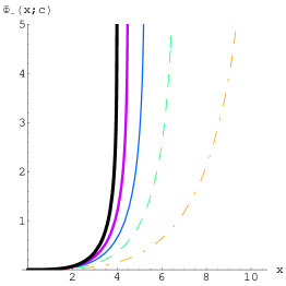
Figure 5: Rate function $\Phi_{-}(x;c)$ for the following values (from left to right) of $c=1,0.8,0.6,0.4,0.2$. See also Figure 3.

We can now compute to leading order the probability that all the eigenvalues are less than the mean value $\langle\lambda\rangle=N/c$. This amounts to putting the barrier at $t=N/c$ in (III.2), which gives $\Phi_{-}\left(\frac{2}{\sqrt{c}}+1;c\right)$. Several numerical values are given in the following table.

$c$	$\Phi_{-}\left(\frac{2}{\sqrt{c}}+1;c\right)$
0.1	0.475802
0.2	0.449162
0.4	0.414592
0.6	0.390245
0.8	0.37104
0.95	0.358805
1	0.355044

Table 2: Some values of the rate function (see text for further explanation).

IV Numerical Results

The formulas (33),(III.1), (51) and (III.2) have been numerically checked on samples of hermitian matrices ($\beta=2$) up to $N=30$, $M=300$ and the agreement with the analytical results is already excellent. We describe in this section the numerical methods and results.

A direct sampling of Wishart matrices up to those sizes is computationally very demanding. We applied the following much faster technique, suggested in [22].

Let $L_{\beta}=B_{\beta}B^{T}_{\beta}$ be the tridiagonal matrix corresponding to:

$$B_{\beta}\sim\begin{pmatrix}\chi_{2a}&\ &\ &\ \\ \chi_{\beta(N-1)}&\chi_{2a-\beta}&\ &\ \\ \ &\ddots&\ddots&\ \\ \ &\ &\chi_{\beta}&\chi_{2a-\beta(N-1)}\end{pmatrix}$$ (57)

$B_{\beta}$ is a square $N\times N$ matrix with nonzero entries on the diagonal and subdiagonal and $a=(\beta/2)M$. The nonzero entries $\chi_{k}$ are independent random variables obtained from the square root of a $\chi^{2}$-distributed variable with $k$ degrees of freedom. It has been proved in [22] that $L_{\beta}$ has the same joint probability distribution of eigenvalues as (II.1). Thus, as far as we are interested in eigenvalue properties, we can use the $L_{\beta}$ ensemble instead of the original Wishart one. This makes the diagonalization process much faster due to the tridiagonal structure of the matrices $L_{\beta}$.

We report the following four plots: the first two (fig. 6 and 7) are for the case $c=1$ and the last two (fig. 8 and 9) for the case $c=0.1$.

In fig. 6, we plot the histogram of normalized eigenvalues $\lambda/2N$ for an initial sample of $3\times 10^{5}$ hermitian matrices ($\beta=2$, $N=M=30$), such that matrices with $\lambda_{\rm max}/2N>\zeta$ are discarded. The barrier is located at $\zeta=3$. On top of it we plot the theoretical distribution (33).

In fig. 8, we do the same but in the case $N=10,M=100$. The barrier is located at $\zeta=14$. The theoretical distribution is now taken from (51).

To obtain the plots in fig. 7 and 9, we generate $\approx 5\times 10^{5}$ $L_{2}$ matrices for different values of $N=7\rightarrow 30$ (or $15$). The parameters $(c,\zeta)$ are kept fixed to the value $(1,3)$ for fig. 7 ($x_{+}=4$) and $(0.1,14)$ for fig. 9 ($x_{+}\approx 17.32$). The constraining capability of those barriers can be estimated by the ratio $\kappa(c,\zeta)=(x_{+}-\zeta)/(x_{+}-x_{-})$, corresponding to the window of forbidden values for the largest eigenvalue. We get $\kappa(1,3)=0.25$ and $\kappa(0.1,14)\approx 0.26$, to be compared with the values of $\kappa(c,\zeta)=(2+\sqrt{c})/4$ for the barrier at the mean value $\zeta=1/c$, which would give respectively $\kappa=0.75$ and $\kappa\approx 0.58$. This relative mildness of the constraint allows us to get a much more reliable and faster statistics in the simulations.

For each value of $N$, we determine the empirical frequency $r(N)$ of constrained matrices as the ratio between the number of matrices whose largest rescaled eigenvalue is less than $\zeta$ and the total number of samples $(5\times 10^{5})$. The logarithm of $r(N)$ vs. the size $N$ is then naturally fitted by a parabola $aN^{2}+bN+\hat{c}$ to test the prediction for $a$ in formulas (III.1) and (III.2).

The best values for the coefficient $a$ of the leading term are estimated as $-0.006153$ ($c=1$) and $-0.0357$ ($c=0.1$), to be compared respectively with the theoretical prediction $\Phi_{-}(1;1)\approx-0.006432$ and $\Phi_{-}(x_{+}-14;0.1)\approx-0.03666$. Despite the relatively small sizes and the $O(N)$ corrections, the agreement is already good.

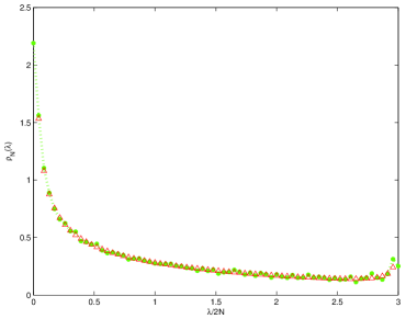
Figure 6: Constrained spectral density $\hat{\varrho}_{N}(\lambda)$ for $N=M=30$. The barrier is at $\zeta=3$. In dotted green the histogram of rescaled eigenvalues over an initial sample of $3\times 10^{5}$ matrices ($\beta=2$). In triangled red the theoretical distribution.

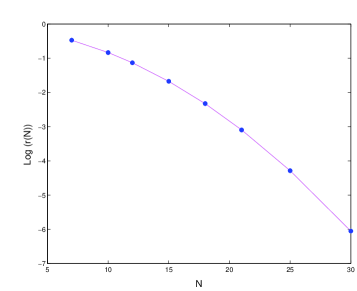
Figure 7: Natural logarithm of the probability that all the rescaled eigenvalues are less than $\zeta=3$ vs. $N$ for the case $c=1$ ($x_{+}=4$). The data points are fitted with a parabola (solid line).

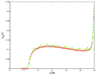
Figure 8: Constrained spectral density $\hat{\varrho}_{N}(\lambda)$ for $N=10$, $M=100$ ($c=0.1$). The barrier is at $\zeta=14$. In dash-dotted green the histogram of rescaled eigenvalues over an initial sample of $5\times 10^{5}$ matrices ($\beta=2$). In triangled red the theoretical distribution.

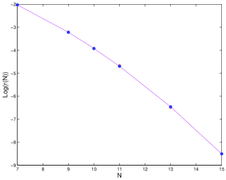
Figure 9: Natural logarithm of the probability that all the rescaled eigenvalues are less than $\zeta=14$ vs. $N$ for the case $c=0.1$ ($x_{+}\approx 17.32$). The data points are fitted with a parabola (solid line).

V Conclusions

In this paper we have studied the probability of atypically large negative fluctuations (with respect to the mean) of the largest eigenvalue $\lambda_{\rm max}$ of a random Wishart matrix. The standard Coulomb gas analogy for the joint probability distribution of eigenvalues allowed us to use the tools of statistical physics, such as the functional integral method evaluated for large $N$ by the method of steepest descent. Using these tools, we have analytically computed the probability of large deviations of $\lambda_{\rm max}$ to the left of its mean. In particular, our main motivation was to compute the probability of a rare event: all eigenvalues are less than the average $\langle\lambda\rangle=N/c$. This implies that the largest eigenvalue itself is less than $\langle\lambda\rangle=N/c$. This question is relevant in estimating the efficiency of the ‘principal components analysis’ method used in multivariate statistical analysis of data. Our main result is to show that, to leading order in $N$, this probability decays as $\sim\exp[-\frac{\beta}{2}N^{2}\Phi_{-}(\frac{2}{\sqrt{c}}+1;c)]$, where $\Phi_{-}(x;c)$ is a rate function that we have explicitly computed. The quadratic, instead of linear, $N$-dependence of the exponential reflects the eigenvalue correlations.

Furthermore, our method allows us to determine exactly the functional form of the constrained spectral density, i.e., the average charge density of a Coulomb gas constrained to be within a finite box $\lambda\in[0,t]$.

All the analytical results are in excellent agreement with the numerical simulations on samples of hermitian matrices up to $N=30$, and the estimates of the large deviation prefactor are already good even for $N\sim 15$.

*

Appendix A Rate function for $c<1$

We evaluate in closed form the action $S(\zeta):=S[\hat{f}^{\star}(x);\zeta]$ (see (III)) for the case $c<1$, where $\hat{f}^{\star}(x)$ is given by (51). The result is in eq. (60).

The rate function $\Phi_{-}(x;c)$ for $c<1$, given by:

$$\Phi_{-}(x;c)=S\left(x_{+}-x\right)-S\left(x_{+}\right)$$ (58)

can be evaluated immediately.

After inserting (51) into (III) and determining $C_{1}$ from (25), we find that $S(\zeta)$ is given by:

$$S(\zeta) =\frac{1}{2}\int_{L_{1}}^{\zeta}\hat{f}(x)xdx-\frac{\alpha}{2}\int_{L_{1}}^{\zeta}\hat{f}(x)\log(x)dx+$$

$$-\int_{L_{1}}^{\zeta}\hat{f}(x)\log(x-L_{1})dx+\frac{L_{1}}{2}-\frac{\alpha}{2}\log(L_{1})$$ (59)

After the substitution $x=(\zeta-L_{1})t+L_{1}$ in the integrals in (A) and some simple algebra, $S(\zeta)$ can be expressed as:

$$S(\zeta)=-\frac{\alpha}{2}\Theta_{1}-\Theta_{2}+\frac{\zeta-L_{1}}{2}\Xi+\frac{L_{1}}{2}-\frac{\alpha}{2}\log(L_{1})$$ (60)

where $\Theta_{k}$ and $\Xi$ are the following functions of $c$ and $\zeta$:

$$\Theta_{k} =\frac{\zeta-L_{1}}{2\pi}\left\{\log(\zeta-L_{1})\left[\frac{A}{\zeta-L_{1}}\mathcal{I}_{0}\left(\frac{L_{1}}{\zeta-L_{1}}\right)-\frac{\pi}{2}\right]+\right.$$

$$+\frac{A}{\zeta-L_{1}}\mathcal{I}_{k}\left(\frac{L_{1}}{\zeta-L_{1}}\right)\left.\right\}$$

$$\Xi =\frac{A}{4}-\frac{3}{16}\zeta-\frac{L_{1}}{16}+\frac{\alpha}{2\pi}\mathcal{I}_{3}\left(\frac{L_{1}}{\zeta-L_{1}}\right)+\frac{1}{2}-\log(2)$$ (61)

The functions $\mathcal{I}_{k}(x)$ are given by the following integrals:

$$\mathcal{I}_{0}(x) =\frac{d}{dx}\mathcal{I}_{3}(x)$$ (62)

$$\mathcal{I}_{1}(x) =\int_{0}^{1}dt\frac{\log(t+x)}{t+x}\sqrt{\frac{t}{1-t}}$$ (63)

$$\mathcal{I}_{2}(x) =\int_{0}^{1}dt\frac{\log t}{t+x}\sqrt{\frac{t}{1-t}}$$ (64)

$$\mathcal{I}_{3}(x) =\int_{0}^{1}dt\log(t+x)\sqrt{\frac{t}{1-t}}$$ (65)

which, following very closely ref. [28] paper I, appendix B, can be computed explicitly in closed form.

The integral $\mathcal{I}_{3}(x)$ (and thus also $\mathcal{I}_{0}(x)$) can be computed by Mathematica^®:

$$\mathcal{I}_{3}(x) =\frac{\pi}{2}\left[1+2x-2\sqrt{x(1+x)}+2\log\left[1+\sqrt{1+\frac{1}{x}}\right]+\right.$$

$$+\log\left(\frac{x}{4}\right)\left.\right]$$ (66)

while $\mathcal{I}_{1}(x)$ and $\mathcal{I}_{2}(x)$ are given in terms of derivatives of hypergeometric functions. More explicit expressions can be given as follows, starting with $\mathcal{I}_{1}(x)$. Exploiting the identity $h^{\lambda}\log h=\partial_{\lambda}h^{\lambda}$, we can rewrite the integral as:

$$\mathcal{I}_{1}(x)=\left[\partial_{\lambda}\int_{0}^{1}dt(t+x)^{\lambda}\sqrt{\frac{t}{1-t}}\right]\Big{|}_{\lambda=-1}$$ (67)

and the integral in (67) can be evaluated in terms of Kummer’s hypergeometric function:

$$\mathcal{I}_{1}(x)=\frac{\pi}{2}\left\{\partial_{\lambda}\left[x^{\lambda}~{}_{2}F_{1}\left(-\lambda,\frac{3}{2};2;-\frac{1}{x}\right)\right]\right\}\Big{|}_{\lambda=-1}$$ (68)

Now, applying the transformation formulas [41] [15.3.7 pag. 559] and evaluating the derivatives of Gamma functions that arise, we finally get:

$$\mathcal{I}_{1}(x) =\frac{\pi}{2}\left[-2\log 4+2~{}\hat{i}_{1}(x)-2\sqrt{\frac{x}{1+x}}\log\left(\frac{4x}{e^{2}}\right)+\right.$$

$$-2\sqrt{x}~{}\hat{i}_{2}(x)\left.\right]$$ (69)

where:

$$\hat{i}_{1}(x) =\left[\partial_{\mu}~{}_{2}F_{1}(1-\mu,-\mu;-\mu+1/2;-x)\right]\Big{|}_{\mu=0}$$ (70)

$$\hat{i}_{2}(x) =\left[\partial_{\mu}~{}(1+x)^{\mu-1/2}~{}_{2}F_{1}(\mu,\mu+1;\mu+3/2;-x)\right]\Big{|}_{\mu=0}$$ (71)

To evaluate $\hat{i}_{1}(x)$ and $\hat{i}_{2}(x)$, we use the series expansion for hypergeometric functions [41] [15.1.1 pag. 556] and upon differentiation we get:

$$\hat{i}_{1}(x)=-\sum_{n=1}^{\infty}B\left(\frac{1}{2},n\right)(-x)^{n}$$ (72)

where $B(v,w)=\frac{\Gamma(v)\Gamma(w)}{\Gamma(v+w)}$ is Euler’s Beta function. Introducing the integral representation of the Beta function:

$$B(x,y)=\int_{0}^{1}dt~{}t^{x-1}(1-t)^{y-1}$$ (73)

into (72) and upon exchanging summation and integral, we arrive with the help of $\sum_{n=0}^{\infty}(-xt)^{n}=(1+xt)^{-1}$ to:

$$\hat{i}_{1}(x)=x\int_{0}^{1}\frac{dt}{\sqrt{1-t}(1+xt)}=2\sqrt{\frac{x}{1+x}}\mbox{arcsinh}(\sqrt{x})$$ (74)

Following the same procedure, we get for $\hat{i}_{2}(x)$:

$$\hat{i}_{2}(x)=\frac{1}{\sqrt{1+x}}\left[\log(1+x)-i_{1}(x)\right]$$ (75)

where $i_{1}(x)$ is defined in ref. [28] as:

$$i_{1}(x)=-2+2\sqrt{\frac{1+x}{x}}\mbox{arctanh}\left(\sqrt{\frac{x}{1+x}}\right)$$ (76)

From (A) we get the final result for $\mathcal{I}_{1}(x)$:

$$\mathcal{I}_{1}(x) =\pi\left\{-\log 4+\sqrt{\frac{x}{1+x}}\left[2\mbox{arcsinh}(\sqrt{x})+\right.\right.$$

$$+2\sqrt{1+\frac{1}{x}}\mbox{arctanh}\left(\sqrt{\frac{x}{1+x}}\right)-\log[4x(1+x)]\left.\left.\right]\right\}$$ (77)

Following the very same procedure as in the previous case, we find for $\mathcal{I}_{2}(x)$:

$$\mathcal{I}_{2}(x)=\pi\left[-\log 4+\sqrt{\frac{x}{x+1}}\left(2\mbox{arcsinh}(\sqrt{x})-\log(x)\right)\right]$$ (78)

Now we compute the limit $c\rightarrow 1^{-}$ in (60) to recover (34). Given that, for $c\rightarrow 1^{-}$, $L_{1}\rightarrow 0$, $\alpha\rightarrow 0$ and $A\rightarrow(\zeta+4)/2$, we have to evaluate the integrals $\mathcal{I}_{k}(x)$ for $x\rightarrow 0$. This gives:

$$\mathcal{I}_{0}(0) \sim\pi$$ (79)

$$\mathcal{I}_{1}(0) \sim-\pi\log 4$$ (80)

$$\mathcal{I}_{2}(0) \sim-\pi\log 4$$ (81)

$$\mathcal{I}_{3}(0) \sim-\frac{\pi}{2}(\log 4-1)$$ (82)

Then, $S[\hat{f}^{\star}(x);\zeta]\Big{|}_{c\rightarrow 1^{-}}\sim\left[-\Theta_{2}+\frac{\zeta}{2}\Xi\right]\Big{|}_{c\rightarrow 1^{-}}=2\log 2-\log\zeta+\frac{\zeta}{2}-\frac{\zeta^{2}}{32}$ as it should (see (34)).

References

- [1] S.S. Wilks, Mathematical Statistics (John Wiley & Sons, New York, 1962).
- [2] K. Fukunaga, Introduction to Statistical Pattern Recognition (Elsevier, New York, 1990).
- [3] For a nice pedagogical introduction to PCA, see L.I. Smith, “A tutorial on Principal Components Analysis” (2002).
- [4] J. Wishart, Biometrica 20, 32 (1928).
- [5] I.M. Johnstone, Ann. Statist. 29, 295 (2001).
- [6] R.W. Preisendorfer, Principal Component Analysis in Meteorology and Oceanography (Elsevier, New York, 1988).
- [7] J.-P. Bouchaud and M. Potters, Theory of Financial Risks (Cambridge University Press, Cambridge, 2001).
- [8] Z. Burda and J. Jurkiewicz, Physica A 344, 67 (2004); Z. Burda, J. Jurkiewicz and B. Waclaw, Acta Physica Polonica B 36, 2641 (2005) and references therein.
- [9] E. Telatar, European Transactions on Telecommunications 10(6), 585 (1999).
- [10] Y.V. Fyodorov and H.-J. Sommers, J. Math. Phys. 38, 1918 (1997); Y.V. Fyodorov and B.A. Khoruzhenko, Phys. Rev. Lett. 83, 66 (1999).
- [11] E.V. Shuryak and J.J.M. Verbaarschot, Nucl. Phys. A560, 306 (1993); J.J.M. Verbaarschot, Phys. Rev. Lett. 72, 2531 (1994).
- [12] K. Johansson, Comm. Math. Phys. 209, 437 (2000).
- [13] S. Maslov and Y.C. Zhang, Phys. Rev. Lett. 87, 248701 (2001).
- [14] Y.K. Yu and Y.C. Zhang, Physica A312, 1 (2002).
- [15] R.A. Janik and M. A. Nowak, J. Phys. A: Math. Gen. 36, 3629 (2003).
- [16] F.J. Dyson, J. Math. Phys. 3 140 (1962).
- [17] V.A. Marcenko and L.A. Pastur, Math. USSR-Sb, 1, 457 (1967).
- [18] F.J. Dyson, Rev. Mex. Fis., 20, 231 (1971).
- [19] O. Bohigas and J. Flores, Rev. Mex. Fis., 20, 217 (1971).
- [20] A. Edelman, SIAM J. Matrix Anal. Appl. 9, 543 (1988).
- [21] P.J. Forrester, Nucl. Phys. B 402, 709 (1993).
- [22] I. Dumitriu and A. Edelman, J. Math. Phys. 43, 5830 (2002);
- [23] A. Edelman and B. Sutton, arXiv:math-ph/0607038.
- [24] D.S. Dean and S.N. Majumdar, Phys. Rev. Lett. 97, 160201 (2006).
- [25] F. Hiai and D. Petz, The semicircle law, free random variables and entropy (American Mathematical Society, Providence, 2000).
- [26] P. Deift, A. Its and I. Krasovsky, arXiv:math.FA/0609451
- [27] M.L. Mehta, Random Matrices, 3rd Edition, (Elsevier-Academic Press) (2004).
- [28] Y. Chen and S.M. Manning, J. Phys. A: Math. Gen. 29 7561 (1996); ibid 27 3615 (1994).
- [29] A.T. James, Ann. Math. Statistics 35, 475 (1964).
- [30] E.P. Wigner, Proc. Cambridge Philos. Soc. 47, 790 (1951).
- [31] C. Tracy and H. Widom, Comm. Math. Phys. 159, 151 (1994); ibid 177, 727 (1996); For a review see Proceedings of the International Congress of Mathematicians, Beijing 2002, Vol. I, ed. LI Tatsien, Higher Education Press, Beijing 2002, pgs. 587-596.
- [32] A. Cavagna, J.P. Garrahan, and I. Giardina, Phys. Rev. B 61, 3960 (2000).
- [33] Y.V. Fyodorov, Phys. Rev. Lett. 92, 240601 (2004) ; Acta Physica Polonica B 36, 2699 (2005).
- [34] L. Susskind, arXiv:hep-th/0302219; M.R. Douglas, B. Shiffman, and S. Zelditch, Comm. Math. Phys. 252, 325 (2004).
- [35] L. Mersini-Houghton, Class. Quant. Grav. 22, 3481 (2005).
- [36] A. Azami and R. Easther, J. Cosmol. Astropart. Phys. JCAP03 013 (2006).
- [37] A.J. Bray and D.S. Dean, arXiv:cond-mat/0611023.
- [38] Y.V. Fyodorov, H-J. Sommers and I. Williams, arXiv:cond-mat/0611585.
- [39] E. Kanzieper, Phys. Rev. Lett. 89 250201 (2002)
- [40] F.G. Tricomi, Integral Equations, (Pure Appl. Math V, Interscience, London, 1957).
- [41] M. Abramowitz and I.A. Stegun, Handbook of Mathematical Functions (Dover Publications,Inc.,New York 1972).