Size distribution and structure of Barchan dune fields

Zusammenfassung

Barchans are isolated mobile dunes often organized in large dune fields. Dune fields seem to present a characteristic dune size and spacing, which suggests a cooperative behavior based on dune interaction. In Duran et al. (2009), we propose that the redistribution of sand by collisions between dunes is a key element for the stability and size selection of barchan dune fields. This approach was based on a mean-field model ignoring the spatial distribution of dune fields. Here, we present a simplified dune field model that includes the spatial evolution of individual dunes as well as their interaction through sand exchange and binary collisions. As a result, the dune field evolves towards a steady state that depends on the boundary conditions. Comparing our results with measurements of Moroccan dune fields, we find that the simulated fields have the same dune size distribution as in real fields but fail to reproduce their homogeneity along the wind direction.

Barchan dunes can be found in fields with low sand availability and unidirectional wind. Above their minimum height, of about one meter, they show regular shapes with simple scaling relations between their height, width, length and volume [Andreotti (2002); Elbelrhiti (2008); Parteli (2007a)]. Moreover, the velocity of one barchan is proportional to the inverse of its width [Hersen (2004a)]. Barchan dunes generally do not appear isolated but instead belong to several kilometer long dune fields, forming corridors oriented along the wind direction. Within these corridors the dunes show rather well selected sizes and inter-dune spacing (see Fig. 1(a)-(d)). However, single barchans alone are intrinsically unstable and they either continuously grow or shrink. This discrepancy leads us to the assumption that, at the statistical level, the behavior and evolution of single dunes results from the interaction with their surroundings typically composed of several thousand dunes [Hersen (2004b); Elbelrhiti (2005)].

Collisions between dunes have been proposed to be one of the processes responsible for the stability of dune fields [Schwämmle (2003); Duran (2005); Hersen (2005a)], another one being dune calving due to wind fluctuations [Elbelrhiti (2005)]. In a recent work, we have already shown that binary collisions alone behave as an additive random process that leads to a stationary Gaussian dune size distribution [Duran (2009)]. We also found that, after adding sand flux exchange into a mean-field model for the evolution of the dune size distribution, the collision-based Gaussian distribution transforms into a new distribution which is similar in shape to a log-normal one [Duran (2009)]. In this mean-field approach however, we ignored the spatially extended character of mobile dune fields. The model, due to its restrictions, does not provide explanation to several issues. For instance, it is still not clear which conditions lead to the different characteristic sizes in different dune field corridors. Therefore, a more realistic approach is used in the work presented here.

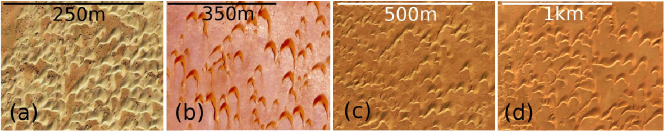
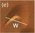
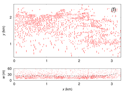
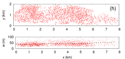
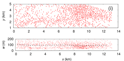
Abbildung 1: (Color online) (a)-(d) Detail of the four measured dune field corridors localized in Western Sahara (wind blows from top to bottom). (e) Dunes are represented by their ‘width line’. (f)-(i) Measured barchan dunes in the four corridors. The $x$ axis is oriented along the wind direction (from left to right) which is also the direction of dune movement. Lower panels show the dune width as function of their $x$-position, where dashed lines indicate the average dune size along the transversal $y$-direction. In all pictures, the North points up.

In this paper, we present further details on dune collisions and proceed to model an entire dune field based on the scaling relations of isolated dunes. These relations were extracted from simulations using a continuous sand flux balance model [Sauermann (2001); Kroy (2002); Schwämmle (2005)]. The aim is to highlight the underlying processes that may lead to size selection in a dune field. In addition, we carry out a quantitative analysis on how the external conditions influence the dune field comparing results from simulation with empirical ones.

The paper is organized as follows: In Sec. 1 we present the measured size distributions and inter-dune spacing distributions for real fields, namely in four barchan dune fields along the coast of Western Sahara (Fig. 1). We show that spatial homogeneity is an ubiquitous feature of dune fields, which present a clear characteristic dune size and a well defined inter-dune spacing. In Sec. 2 we start by describing a simulation of a whole dune field using a continuous sand flux balance model which reproduces qualitatively the real dune field. Then, observing that the number of dunes is too small to be statistically relevant, we present in Sec. 2.1 a model for the internal dynamics of the dune field taking into account only binary collisions. In Sec. 2.2, this description turns out to be oversimplified, motivating the further inclusion of both, the simple rules for barchan collisions and the sand flux balance on isolated dunes, and therefore introducing a simplified model of a large dune field. Simulations of such model are presented in Sec. 3, providing scaling relations between the spatial distribution, the size distribution and the boundary conditions. Finally, the conclusions are presented, with additional discussions on dune calving [Elbelrhiti (2005)] in the scope of the stability of dune fields.

1 Empirical data and data analysis

1.1 Data sets

The Moroccan desert in Western Sahara contains the longest barchan dune fields on Earth. Satellite images of these deserts are good sources for statistical input to calculate the size distribution of sand dunes. In Ref. [Duran (2009)] the distribution functions of dune sizes have already been presented. Here we are particularly interested in the spatial distribution of the dunes.

In Western Sahara, barchan dunes develop under a strong uni-directional wind in tens of kilometers long corridors with, at least over reasonable large regions, a characteristic dune size and a homogeneous dune distribution (Fig. 1(a)-(d)).

It has been shown, both from models [Sauermann (2001); Hersen (2004a)] and measurements [Sauermann (2000); Elbelrhiti (2005, 2008)], that the velocity of barchan dunes as well as height, area and volume, are well characterized by their width $w$ solely. Therefore, we only measure the width and position of more than $5,000$ dunes corresponding to four dune field corridors between Tarfaya and Laayoune (Morocco) using satellite images from GoogleEarth, with one meter per pixel resolution.

The four dune fields illustrated in Fig. 1 have respectively $1295$, $1113$, $1947$ and $1630$ barchan dunes, covering areas of $\sim 3,7,12$ and $60$ km² and with average dune sizes of $17$m, $27$m, $42$m and $86$m respectively. The width line is defined as the largest distance between the dune horns, as illustrated in Fig. 1e. Figure 1(f)-(i) shows the four measured dune fields, where each barchan is represented by its ‘width line’ as a function of its $x$-coordinate (downwind distance) along the corridor. The downwind direction in a barchan dune field is given by the horns of the dunes[Sauermann (2001)].

The errors of the measured widths and location of the dunes are of the same order as the resolution of the satelite image, namely $1$m, which is in most cases neglegible in comparison with the width. Therefore we do not consider such errors here. In the cases where only one horn is visible, the width is taken assuming the dune to have a symmetrical shape. Calving is therefore not considered in our analysis. Further, a set of overlaping dunes (see Fig. 4) is either neglected or taken as a single dune in case one dune is much larger then the other ones.

From Fig. 1, one sees that there is no clear trend in the spatial distribution at the scale of the image resolution. One also notes that, while between corridors a wide variety of dune widths is observed, ranging from 5 m to 250 m, together with different dune concentration, each corridor per se has a characteristic dune size.

1.2 Features of empirical data

All four measured dune fields have a common underlying size distribution function, close to a log-normal and is well reproduced by a master equation that balances the dune growth due to sand flux exchange with the sand redistribution due to collisions between dunes [Duran (2009)].

While the size distribution can be fully described only by the mean size (see [Duran (2009)]), what determines the characteristic size at different corridors is still unknown.

The spatial distribution of dunes provides additional information beyond the size distribution, namely about the sand distribution within the field and the total amount of sand transported through it [Duran (2009)].

We define the inter-dune spacing, $L(w)$, as the characteristic distance between a dune of width $w$ and its neighbors,

$$L(w)\equiv\sqrt{A_{f}(w)}\leavevmode\nobreak\ ,$$ (1)

where $A_{f}(w)$ is the sand-free area around the dune. This area is computed as follows. Each dune is connected to its four nearest neighbors, one at each quadrant of a Cartesian coordinate system centered at the dune, composing a planar dune network as sketched in Fig. 2. After searching the nearest neighbors of each dune, the edges joining the neighbors of one particular dune compose a polygon with area $A_{p}$. The sand-free area is simply $A_{f}=A_{p}-\omega^{2}$, i.e. the remaining area that is left after subtracting the area of the dune, approximated as $\omega^{2}$.

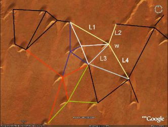
Abbildung 2: (Color online) Dune field planar network. The neighborhood of a dune of width $w$ is defined by its nearest neighbors in each of the four quadrants placed at a distance $L_{1}$, $L_{2}$, $L_{3}$ and $L_{4}$, respectively.

As previously reported [Duran (2009); Hersen (2004b)], we find that the spacing between dunes takes well-selected values within the same field. Additionally, the inter-dune spacing $L$ shows no clear trend as a function of the dune size $w$; its mean value $\bar{L}$ is nearly constant over the whole width range and only depends on the selected dune field.

This independence between dune size and dune spacing is not only a consequence of the uniformity of the spatial distribution of dunes but also a special feature of barchan dune fields deeply rooted in the dynamics of dune size selection and their spatial distribution. For instance, on static dune fields, such as longitudinal or star dune fields, the inter-dune spacing scales with the dune size, i.e. larger dunes are surrounded by larger empty space, due to the way sand is redistributed among the dunes. In static dune fields, since the annual average of the relative motion between dunes is almost zero, they change their size only by their influx-outflux balance. Therefore, due to mass conservation, a dune accumulates sand and grows only by extracting sand from its neighboring dunes that shrink.

In barchan dune fields, dunes are mobile and therefore can collide with each other. Next, we present arguments to strengthen the hypothesis that the interchange of sand due to dune collisions destroys any simple correlation between dune size and inter-dune distance and leads to the observed spatial uniformity.

2 Data modeling: simulating the dune field

Many barchan dune fields arise from the accumulated sand in the sea shores. For isolated dunes, the sand flux exchanged with the sea shore would promote their continuous growth. Other mechanisms at the dune field scale, such as dune collisions, combined with sand exchange processes between dunes and with their surroundings, enable their stabilization at the dune field scale [Duran (2009)].

To address the problem of dune field stabilization, we start in this section with numerical simulations of an entire dune field using a continuous sand flux balance model [Sauermann (2001); Kroy (2002); Schwämmle (2005)]. This model has already been successfully applied to explain the formation and dynamics of isolated barchan dunes [Sauermann (2003); Schwämmle (2005); Parteli (2007a, b); Duran (2010)], the formation of transverse dunes [Schwämmle (2004)] and the transition from barchan to parabolic dunes through vegetation growth [Duran (2006)]. A detailed description of the model can be found in Refs. [Schwämmle (2004); Parteli (2007a); Duran (2010)].

The model considers a uniform sand bed over a non-erodible surface in the center of the field, as illustrated in Fig. 3a. Periodic boundary conditions are implemented in both the downwind direction and the direction perpendicular to it.

At the beginning, transversal instabilities appear all over the sand bed propagating downwind until the whole bed is fragmented into transversal dunes (Fig. 3b). Once the sand between the dunes is completely eroded, transversal dunes become unstable and split into two separated lanes of barchan dunes (Fig. 3c). Difference in dune size leads to collisions between barchan dunes that together with the flux exchanged between them act as a size selection mechanism, leading to a stationary size distribution (Fig. 3d). This last stage is the one typically observed in real dune fields (see Figs. 4), characterized by the emergence of clusters of colliding dunes and alternating localizations of consecutive barchans.

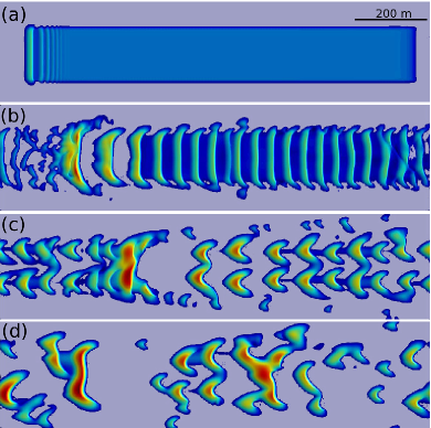
Abbildung 3: (Color online) Snap shots of the dune field evolution beginning with a uniform sand bed under periodic boundary conditions. Wind blows from left to right.

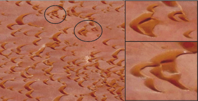
Abbildung 4: (Color online) Collisions between barchan dunes are ubiquitous in this Moroccan dune field. On the right side are two examples.

While the simulated field in Fig. 3 reproduces the main features of a real one, it has typically $\sim 30$ dunes in its stationary state, instead of the $\sim 1500$ dunes observed in the real fields. Larger number of dunes imply a large computation effort, since the model reproduces the full shape and dynamics of each dune.

For a proper statistical characterization of size and spatial distributions in dune fields we propose an alternative model. We start in Sec. 2.1 by describing how collisions between dunes may lead to the selection of a characteristic dune size within the field and in Sec. 2.2 we combine dune collisions with the full dune motion and the sand-flux exchanged between them.

2.1 Size regulation by dune collisions

To understand physically the dune size distribution one must take into account the dynamical processes that govern the growth of single dunes. The intrinsic instability of barchan dunes under an incoming sand flux leads to an increase of the largest dunes in the field whereas the smaller ones shrink until they disappear [Duran (2010); Hersen (2004b, 2005a)]. Hence, the mean size of the dunes should grow with the distance from the beginning of a field. Nevertheless, in many dune fields the sizes saturate. Two mechanisms have been proposed to avoid unlimited dune growth: instability of large dunes due to changing wind directions [Elbelrhiti (2005)] and collisions between dunes [Schwämmle (2003); Duran (2005); Hersen (2005a)]. Here, we concentrate on the second mechanism.

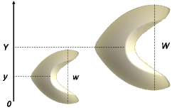
Abbildung 5: (Color online) Sketch of the initial state of a binary collision between two barchan dunes of sizes $w$ and $W$, and centered at $y$ and $Y$, respectively.

Collisions are ubiquitous in dune fields (see Fig. 4) due to the relatively broad range of different velocities which obey in general $v\sim 1/w$ for single dunes [Hersen (2005b)]. Due to this dependence of their velocity on their size, the dune that collides onto a second one must be smaller than the latter one. This process has been observed several times [Besler (1997, 2002)] but was not understood until recently. The large temporal scale of such a process makes it difficult to observe the final state after such a collision.

Simulations using the continuous dune model were carried out to understand what happens when two dunes collide with each other. Figure 6 shows that, after the smaller barchan bumps onto the larger one, a hybrid state is formed where the two dunes melt into a complex pattern. Depending on the initial relative size $r_{i}\equiv\frac{v}{V}$, where $V$ is the volume of the large barchan and $v$ the volume of the small one, and their lateral offset $\theta_{i}\equiv\frac{|Y-y|}{W/2}$, where $Y$ and $y$ are the coordinates of the crest of the large and the small dune in the lateral direction transverse to their movement, respectively, and $W$ is the width of the larger dune (see Fig. 5), four different situations can emerge after collision: coalescence, where only one dune remains, breeding (Fig. 6, ‘b’) and budding (Fig. 6, ‘bu’) where two dunes leave the larger one, and solitary wave behavior (Fig. 6, ‘s’) where the number of dunes remains two after the collision. These different final situations provide mechanisms to redistribute sand and thus to avoid the continuous growth of dunes in a dune field. Similar occurrences can be observed in experiments with sub-aqueous barchans [Endo (2004)].

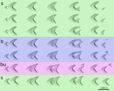
Abbildung 6: (Color online) Snap shots of the time evolution of binary collision for $\theta_{i}=0.2$ and volume ratios (from top to bottom): $r_{i}=0.06$, $0.08$, $0.12$, $0.17$ and $0.3$. Letters and colors distinguish the different results after collision. Notice that the smallest volume ratio $r_{i}=0.06$ used for the set of simulations, is large enough to avoid dune coalescence.

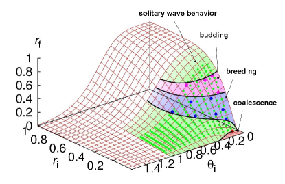
Abbildung 7: (Color online) Sketch of the morphological phase diagram for binary collisions. The volume ratio $r_{f}$ after the collision is plotted as a function of the initial offset $\theta_{i}$ and the initial volume ratio $r_{i}$. Dots represent simulation results.

Next we construct a heuristic set of collision rules based on simulations with the continuous dune model described above. These collision rules provide the same statistical output as the continuous model, enabling to treat pairs of dunes as single objects which interact whenever the initial relative lateral offset between them is $\theta_{i}<1$. Together with the initial lateral offsets we also consider the corresponding initial volume ratio $r_{i}$.

The morphological phase diagram of binary collisions is schematically shown in Fig. 7 in terms of the final volume ratio $r_{f}$ as a function of the initial volume ratio and lateral offset. For simplicity only conservative collisions are included, i.e. we assume that after the collision the summed volume of the ejected dunes corresponds to only one characteristic dune. We notice that the lateral positions of both dunes change after the collision, but no simple rule could be found. Therefore, a new mutual lateral offset is tossed for each collision. Appendix A contains all details concerning the rules for collisions.

Using the diagram in Fig. 7 for taking the final volume ratio $r_{f}$ after one collision, we next consider the simplest approach to a dune field model, namely, a system that consists of a large number of dunes, characterized only by their width, which interact exclusively through collisions between them. For each collision two dunes are taken randomly from the field to collide. This is repeated every iteration as many times as the number of dunes in the field.

Within this framework, we study the evolution of the dune size distribution $P_{col}(w)$ in the entire field in order to check if the macroscopic behavior of the system approaches a steady state.

We have shown that [Duran (2009)] the size distribution function converges toward an absorbent state with a stable Gaussian-like distribution with mean width $\langle w\rangle_{col}$. The total mass of all dunes is conserved with the exception of a negligible amount due to the small dunes removed from the field. Therefore, the mean dune size $\langle w\rangle_{col}$ is determined by the average volume $\langle V\rangle$.

Since it is a Gaussian, the size distribution $P_{col}(w)$ only depends on the average volume of the field $\langle V\rangle$, namely

$$P_{col}(w)=\frac{1}{\sqrt{2\pi}\,\sigma_{col}}\exp{\left[-\frac{(w-\langle w\rangle_{col})^{2}}{2\,\sigma_{col}^{2}}\right]}.$$ (2)

Furthermore, the mean square deviation $\sigma_{col}$ is proportional to the mean dune size $\langle w\rangle_{col}$ [Duran (2009)].

From our findings above one concludes that collisions alone act as a random additive process and are able to select a characteristic dune size from a given initial condition. However, this mean-field approach doesn’t give information about neither the spatial distribution of the dunes nor the role played by the positions of the dunes on the actual collisions.

2.2 A simplified dune field model

Calculations of very large dune fields are still difficult because of high computational costs. The continuous dune model reproduces the dune evolution at the scale of the saturation length (typically $\sim 1$m) and thus is extremely expensive in terms of running time for large dune field simulations. One way out would be to consider a simplified ‘coarse-grained’ dune model, where dunes are themselves the basic objects. For that purpose we use the collision rules obtained above together with the rules for the motion and evolution of barchans obtained from continuous simulations [Duran (2010)].

This effective model considers a barchan dune field with constant unidirectional wind, a maximum length $x_{max}$ in the wind direction and width $y_{max}$ and fed by small barchans entering upwind into the field. The width $w_{0}$ of the incoming dunes is constant and they enter at a rate $\nu$ –number of incoming dunes per time step. Their $y$-position is randomly distributed.

Abbildung 8: The model for barchan dune fields. Illustration of the set of operations executed at each time step.

Each dune is characterized by its width $w$ and its coordinates in the field, $x\in[0,x_{max}]$ and $y\in[0,y_{max}]$. In each iteration the dunes change their size and position due to the sand flux balance and collisions. Next, a detailed description of the algorithm is presented. A graphical illustration of the different steps during one iteration is given in Fig. 8.

Tabelle 1: Model parameters

Dune parameters
Dune outflux-influx relationship, slope:	$a=0.45$
Dune outflux-influx relationship, offset:	$b=0.1$
Proportionality between volume and cubic width:	$c=0.017$
Dune velocity constant:	$\alpha=50$
Model parameters
Time step:	$\Delta t=0.001$ yr
Maximum number of iterations:	$T=10^{6}\equiv 10^{3}$ yrs
Field width:	$y_{max}=3$ km
Field length:	$x_{max}=20$ km
Saturated flux:	$Q=300$ m2/yr
Dune field influx:	$q_{f,in}=0$
Surface density:	$\rho_{0}$ (variable)
Size of incoming dunes:	$w_{0}$ (variable)
Rate of incoming dunes:	$\nu$ (variable, Eq. (7))

We start by the sand flux process. The dune’s influx $q_{in}$ determines the volume alteration of a dune and so its new width $w$. Following Ref. [Duran (2010)], the mass balance on a barchan dune can be well approximated as

$$\dot{w}=\frac{Q\delta}{3c\,w},$$ (3)

where $c$ is the proportionality constant between the dune volume and the cubic power of the width [Duran (2010)], $\delta\equiv(q_{in}-q_{out})/Q$ denotes the flux balance on the dune, with $q_{in}$ and $q_{out}$ the dune influx and outflux, respectively and $Q$ is the saturated flux. Since the normalized outflux can be written as

$$\frac{q_{out}}{Q}=a\frac{q_{in}}{Q}+b,$$ (4)

where $a$ and $b$ are the slope and offset in the outflux-influx relation [Duran (2010)], the flux balance reads $\delta=(1-a)q_{in}/Q-b$. Table 1 indicates the particular values used in our simulations.

From time $t$ to $t+\Delta t$ the dune evolves in time with a width given by the integration of Eq. (3), namely

$$w(t+\Delta t) = \sqrt{w^{2}(t)+\frac{2Q\delta}{3c}\Delta t}$$ (5)

Meanwhile, the dune moves forward a distance $x-x_{0}$ that results from the integration of the dune velocity-width relationship, $v=\alpha Q/w$ [Duran (2010)]. From Eq. (3), this relation becomes $v=3c\alpha\dot{w}/\delta$. After integration, it yields

$$w(x)=w(x_{0})+\frac{\delta}{3c\alpha}(x-x_{0})\leavevmode\nobreak\ ,$$ (6)

which predicts a linear change of the dune size with the distance it moves.

The dune contribution to the sand flux in the field is as follows. From the normalized outflux in Eq. (4), the total sand flux out of a dune of width $w$ is $q_{out}w$, where the flux is assumed to be homogeneously distributed along the dune width, due to diffusion processes. This is in fact a simplified picture of what happens in real dunes. There, the sand leaves the horns with an intensity of nearly the saturated flux $Q$ and the remaining part of the dune is dominated by the dune’s slip face from where almost no sand leaves [Kroy (2002)]. Thus, on average $q_{out}w$ is a good approximation for the total sand flux.

The updated flux field determines the influx on the next dune. This dune again updates the flux field by replacing the influx at the corresponding $x$-position by its outflux while simultaneously either changing its size or being eliminated from the field.

After updating all dunes according to the actual sand flux of the field at their position, we look if their new positions and sizes lead to collisions.

First, we check if a dune overtakes another one or if they overlap in their lateral extension. When they overlap, we apply the collision rule, derived in the previous section, and calculate the new widths and positions. Therefore, collisions are taken as instantaneous and every time two dunes collide we select a small random lateral offset.

At the end of each iteration, incoming dunes are generated and positioned at the beginning of the field, $x=0$.

3 Results

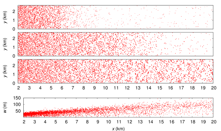
Abbildung 9: Top, three characteristic stages of the evolution of a dune field at 20 yr ($2\times 10^{4}$ steps), 50 yr ($5\times 10^{4}$ steps) and the steady state after about 100 yr ($10^{5}$ steps). Dunes move from left to right and are represented by the ‘width line’, i.e. a line centered in the center of mass of the dune and with a length equal to the dune width. Bottom, dune width $w$ as function of its distance downwind at the steady state.

In this Section we present the main results from simulations for different dune input rates $\nu$ and sizes $w_{0}$ using the model, described in the previous section.

Since the incoming dunes are randomly distributed along the input boundary $x=0$ we impose the density $\rho_{0}$ of the incoming dunes instead of the input rate $\nu$. From the definition, $n$ dunes of width $w_{0}$ uniformly distributed in an area $A=y_{max}\Delta X$ have a surface density $\rho_{0}\equiv(n\,w_{0}^{2})/(y_{max}\Delta X)$ where $y_{max}$ is the field width and $\Delta X=v\,\Delta t$ is the distance covered by dunes with velocity $v=\alpha Q/w_{0}$ during a time interval $\Delta t$ equal to one time step. Since by definition the input rate is $\nu=n/\Delta t$, the dune density becomes

$$\rho_{0}=\nu\frac{w_{0}^{3}}{\alpha Qy_{max}}$$ (7)

where the parameters are given in table 1. We apply periodic boundary conditions in the direction perpendicular to the wind.

Figure  9 (upper panel) shows the evolution of a typical dune field with a high density ($\rho_{0}=0.42$) of about 2 m high incoming dunes ($w_{0}=20$ m). The dune field invades the whole simulated area and finally reaches a steady spatial distribution. In general, along the wind direction, the spatial distribution is not uniform, dunes become progressively sparse, and at the same time the dune size increases (Fig. 9, bottom). As will be shown below, this coarsening is a direct consequence of the -unstable- flux balance and differs from the homogeneous distribution of real dune fields (see Fig. 1).

In spite of this difference, the global dune size distribution in the simulated fields actually corresponds to the measured ones, and thus are also well described by the analytical mean-field model [Duran (2009)] (Fig. 10). Therefore, the Gaussian distribution induced by the high rate of collisions at the beginning of the field, is gradually skewed toward large sizes due to the coarsening. However, the interaction dynamics we use is too simple and does not capture the fragmentation process that should compensate coarsening and lead to a homogeneous distribution. This shortcoming is discussed in the next section, along with some ideas how to overcome it.

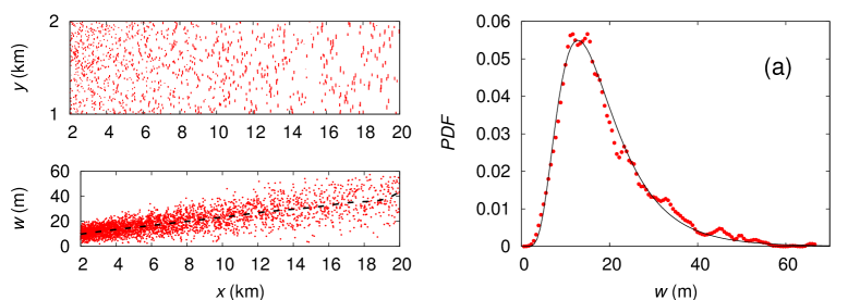
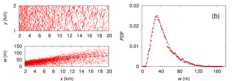
Abbildung 10: Dune width distribution of two simulated dune fields together with a snap shot of the field in the stationary state (top left) and the downwind dune size distribution (bottom left). In the distribution function, dots are measured points and the line is the analytical model. The boundary conditions are: (a) $w_{0}=10$ m, $\rho_{0}=0.18$, and (b) $w_{0}=20$ m, $\rho_{0}=0.42$.

Abbildung 11: Collapse of the normalized local mean dune width $w(x)/\langle w\rangle$ as function of the downwind distance $x$ (symbols) for different boundary conditions, e.g. a different input dune density $\rho_{0}$. The solid line corresponds to the linear fit. $\langle w\rangle$ is the mean dune size in the whole field.

Abbildung 12: The local dune density $\rho(x)$ as function of downwind distance remains constant along the whole field independent of the boundary conditions. In the figure $\rho(x)$ is normalized by the total density $\rho$

Abbildung 13: Normalized local dune density $n(x)\equiv N(x)(x_{max}/dx)/N$, where $N(x)$ is the fraction of the total number of dunes $N$ placed between $x-dx$ and $x+dx$, as function of the downwind distance $x$ for different input dune densities (symbols). The solid line corresponds to the $1/w^{2}(x)$ fit (see text). Inset: the local dune mean size $w(x)$ scales as $\langle w\rangle/\sqrt{n(x)}$ (solid line).

As shown in Fig. 11 the local average dune size $w(x)$ increases linearly with the downwind distance $x$. The width $w(x)$ is defined as the average size inside an area $[x-dx/2,x+dx/2]\times[0,y_{max}]$, where $dx$ is the length of the averaging window. Surprisingly, this increasing average of the dune size is not affected by the collision dynamics and simply follows the flux balance result given by Eq. (6). After normalizing the dune size by the mean width $\langle w\rangle$, all curves corresponding to different input dune densities $\rho_{0}$ collapse. This linear increase has also been observed in small real dune fields in Morocco and is apparently related to the initial states of the dune fields [Elbelrhiti (2008)].

Following Eq. (6), from the slope of the spatial increase of the mean size $w(x)$ it is possible to calculate the average inter-dune balance term $\langle\delta\rangle$. Based on the definition $\langle\delta\rangle\equiv(1-a)\langle q_{in}/Q\rangle-b$ and the values $a\approx 0.45$ and $b\approx 0.1$, one can then estimate the average normalized influx inside a dune field, $\langle q_{in}/Q\rangle$ which is in the range $1.04-1.17\,q_{c}/Q$. Therefore, the average influx is very close to the equilibrium influx $q_{c}/Q$ at which dune outflux equals dune influx.Furthermore, from Fig. 11 the difference $\langle q_{in}/Q\rangle-q_{c}/Q$ as expected, scales with the ratio $\langle w\rangle/L_{c}$, i.e. a higher mean dune influx implies a larger mean size.

Another interesting result that follows from the conservation of sand inside the field, is that the local dune density $\rho$ remains constant along the field (Fig. 12). The local dune density is defined as $\rho(x)=A_{s}(x)/A$, where $A_{s}(x)$ is the fraction of the local area $A=dx\times y_{max}$ covered by dunes. Since $A_{s}(x)\approx N(x)w^{2}(x)$, with $N(x)$ as the local dune number with mean size $w(x)$, it follows that the local concentration of dunes scales as $1/w^{2}(x)$ (Fig. 13).

From the definition of the dune density $\rho\approx N\langle w\rangle^{2}/(N\langle w\rangle^{2}+A_{L})$ with $N$ being the number of dunes and $A_{L}$ being the free total area between dunes, and taking into account that $A_{L}$ scales with the mean inter-dune spacing $\bar{L}$ as $\bar{L}^{2}$, one may write,

$$\rho=\frac{1}{1+\gamma\left(\frac{\bar{L}}{\langle w\rangle}\right)^{2}}\leavevmode\nobreak\ .$$ (8)

Figure 14 shows the densities of both, measured and simulated dune fields, with circles and bullets respectively, as a function of the relative inter-dune spacing $\bar{L}/\langle w\rangle$. The solid line indicates a least square fit with the functional form in Eq. (8) with one single parameter $\gamma$. All points from empirical and simulated data are well predicted by Eq. (8) whose fit yields a value for the fitting constant $\gamma\sim 0.6$. Figure 14 clearly strengthens the theoretical derivations above, showing that the density of dunes is approximatelly uniform and depends exclusively on the relative inter-dune spacing.

Abbildung 14: Dune density $\rho$ as a function of the relative inter-dune spacing $\bar{L}/\langle w\rangle$ for the real dune fields in Fig. 1 ($\circ$), simulated dune fields ($\bullet$)

and the fit when both are taken into account (solid lines).

Making use of our first picture how the field properties relate to each other, we finally address the open question of why different dune fields may have different densities and characteristic dune sizes. From the analysis of the simulated fields we found that the density and average width are, in fact, dependent on the boundary conditions, namely the input density $\rho_{0}$ of dunes and the corresponding width $w_{0}$, determining the input of dunes into the field.

For the simulated dune fields, Fig. 15a suggests the following relation for the average width,

$$\langle w\rangle=\left(\bar{W}\rho_{0}w_{0}\right)^{1/2},$$ (9)

where $\bar{W}\sim 225$ m is a threshold length determining whether the mean dune size in the field is smaller or larger than the size of incoming dunes.

In this context, when incoming dunes are smaller than the product $\bar{W}\rho_{0}$, their density is high enough to enhance the sand exchange through flux balance and they will grow, increasing the mean dune size. Otherwise, if the incoming dunes are larger than $\bar{W}\rho_{0}$, then their density is too low compared to their size and they cannot establish sufficient sand exchange between them. In this case they will shrink inside the dune field, decreasing the mean dune size.

Finally, the dune density $\rho$ in the field, plotted in Fig. 15b, scales with the initial density $\rho_{0}$ as

$$\rho=\rho_{0}-\rho_{c}\leavevmode\nobreak\ ,$$ (10)

where $\rho_{c}\approx 0.12$ is a critical density below which the incoming dunes do not receive enough sand to persist and thus disappear. Equation (10) can also be understood from volume conservation: since the amount of sand blown into the field, given by $\rho_{0}$, has to be shared between the dunes, described by $\rho$, and the sand in the aerial layer, one expects that $\rho<\rho_{0}$ when the corresponding difference $\rho_{c}$ denotes the density associated to the aerial sand flux.

Abbildung 15: (a) The average width $\langle w\rangle$ as a function of the product between the incoming dune density $\rho_{0}$ and the width $w_{0}$ of the incoming dunes at the boundary. (b) The final stationary density $\rho$ of the dune field as function of the initial density $\rho_{0}$ at the boundary. Note that below $\rho_{c}$ (black circle) no dune field formation can be attained.

We presented measurements of dune width and position in four real dune fields in Morocco, finding a common underlying size distribution and a clear spatial homogeneity. The uniformity of the spatial dune distribution gives strong evidence that dune collisions are a non-negligible dynamical effect.

In order to reproduce the morphology of dune fields we revisited two previous models, namely a continuous sand flux balance model and a mean-field model. The continuous model, despite being unable to simulate dune fields as large as the observed ones, provided accurate statistics for the different types of binary collisions between dunes and confirmed the relevance of dune collisions during the whole field evolution. The mean-field model uses the dune collisions output from the continuous model to introduce heuristic dune collision rules, from which the observed dune size distributions are obtained.

We introduced a simplified model for dune fields that treats dunes as simple elements described by their width. This model includes simple collision rules and exchanged flux in order to account for the interaction between dunes and uses basic relations between dune volume, area, outflux and velocity in terms of dune width. As a result, the dune size distribution compares very well with the measured ones and converges to a spatially stationary distribution as observed in real dune fields.

In contrast to measured real fields, the simulated ones are not spatially uniform. A possible explanation could be that the collision model we use is too simple. Indeed, we assume that during collisions, the number of dunes does not increase. However, simulations of binary collisions show a rather different picture, where quite often a colliding dune is unstable and splits into two, a situation called either breeding or budding. Such ‘multiplicative’ collisions may counterbalance the coarsening effect of the sand flux exchange, thus leading to a uniform steady distribution. This is a particularly important point since it has been also observed that real barchan collisions may lead to dune fragmentation into several small dunes [Elbelrhiti (2005)]. Such fragmentation appeals for a different data extraction, since it implies a width of a potentially asymmetric dune. Further, as stated above in Sec. 3, if the dune field is small enough, as it is the case of some Moroccan dune fields, a linear increase of dune size with downwind distance can be observed. To address these two points, a comparison to these smaller fields must be done, which is out of our scope. First, because, as explained in Sec. 1, our data does not allow a resolution fine enough to distinguish the formation of smaller dunes and dunes in hybrid states such the ones in Fig.4. Second, because the linear increase of dune size does not hold when collision enter into play, which occurs for sufficiently large dune fields, such as the ones addressed in this study.

Another possible contribution for the non-uniform spatial distribution at large field distances concerns the time scales taken for collisions. For both the mean-field approach presented in [Duran (2009)] as well as our effective model, the collision time-scale is much shorter than the characteristic time-scale of the evolving dune field. The continuous numerical model for the dune field however presents a collision time-scale of the same order as the typical time of dune motion. Considering the fact that collision are not instantaneous and therefore during one collision both dunes move all together with a lower velocity - proportional to the inverse of the sum of their widths - one expects that considering instantaneous collision, while simplifying an analytical approach, may also contribute for the non-uniformity of the obtained dune field. Additional investigations should be made to clarify these points.

We also found that the condition at the dune field input boundary, namely the size of incoming dunes and their density, are sufficient to determine the main properties of dune fields, the dune density $\rho$, the inter-dune spacing $\bar{L}$ and the mean size $\langle w\rangle$.

It should be emphasized that the input boundary exerts a direct influence onto the dune field whereas other quantities like wind strength apparently do not have much impact. An additional mechanism outside the scope of this manuscript is dune calving: Strong seasonal winds lead to the instability of large dunes in the Moroccan barchan field [Elbelrhiti (2005)] and this instability leads to dune calving which prevents continuous dune growth.

Anhang A

Heuristic rules for binary dune collisions

In this Appendix we describe in detail the collision rules discussed above in Sec. 2.1 from which the plot in Fig. 7 is obtained.

We consider two dunes with different sizes, $w_{M}>w_{m}$. The largest dune is located at $(x_{M},y_{M})$ and the smallest one at $(x_{m},y_{m})$. The $x$-axis is taken parallel to the wind and thus dune widths align parallel the $y$-axis (Fig. 5). The initial offset is therefore

$$\theta_{i}=2\frac{|y_{M}-y_{m}|}{w_{M}}$$ (11)

and the initial volume ratio is given by

$$r_{i}=\left(\frac{w_{m}}{w_{M}}\right)^{3}.$$ (12)

For two dunes to interact, it is necessary that the smallest (fastest) dune overtakes the largest one. When this happens the two dunes collide if their width overlap, namely $y_{M}+\tfrac{1}{2}w_{M}>y_{m}-\tfrac{1}{2}w_{m}$ and $y_{M}-\tfrac{1}{2}w_{M}<y_{m}+\tfrac{1}{2}w_{m}$. It is easy to verify that this latter condition implies $\theta_{i}<\theta_{c}\equiv 1+r_{i}^{1/3}$.

After a collision, the volume ratio $r_{f}$ can be approximately expressed by the phenomenological equation

$$r_{f}(\theta_{i},r_{i})\approx\left[1-e^{-A(\theta_{i})\left[r_{i}-r_{0}(\theta_{i})\right]^{4/3}}\right]\leavevmode\nobreak\ ,$$ (13)

valid for $r_{i}>r_{0}(\theta_{i})$. This condition takes into account that there is a minimal relative size $r_{0}$ of the incoming dune below which no new dune leaves, i.e. coalescence occurs. The coalescence threshold $r_{0}$ is found to be function of the initial lateral offset $\theta_{i}$, and after fitting the numerical data it can be approximated by,

$$r_{0}(\theta_{i})\approx 0.12\,e^{-(\frac{\theta_{i}}{0.4})^{2}}-0.05\leavevmode\nobreak\ .$$ (14)

This equation also defines a maximum offset $\theta_{i}^{M}\sim 0.4$ above which no coalescence occurs.

On the other hand, the term $A(\theta_{i})$ represents the sensibility of the final volume ratio $r_{f}$ to the initial offset and volume ratio, and using the numerical data it can be approximated as

$$A(\theta_{i})\approx 10\left(e^{-(\frac{25\theta_{i}}{9})^{4/3}}-e^{-(\frac{25\theta_{c}}{9})^{4/3}}\right),$$ (15)

We assume for simplicity that in all collisions there are either one (as for coalescence) or two dunes as output (as for solitary wave behavior). The width of the larger one is:

$$\tilde{w}_{M}=\left(\frac{w_{M}^{3}+w_{m}^{3}}{1+r_{f}}\right)^{(1/3)}$$ (16)

with $r_{f}$ given by Eq. (13). The final offset $\theta_{f}$ of the outcoming dune is taken randomly from the interval $[-1,1]$ (see Sec. 2.1).

Coalescence occurs when $r_{i}<r_{0}$ (see Eq. (14) above). For larger $r_{i}$ and $\theta_{i}$, the slip face survives for longer time, mass exchange becomes relevant, and a small barchan is ejected from the main dune. We call this process solitary wave behavior. The final width of the smaller dune is

$$\tilde{w}_{m}=r_{f}^{1/3}\tilde{w}_{M}.$$ (17)

The final offsets of both dunes is

$$\Delta y_{M} = \frac{r_{f}\theta_{f}}{1+r_{f}}-\frac{r_{i}\theta_{i}}{1+r_{i}}$$ (18a)

$$\Delta y_{m} = \frac{\theta_{i}}{1+r_{i}}-\frac{\theta_{f}}{1+r_{f}}$$ (18b)

and the corresponding $y$-coordinates are

$$\tilde{y}_{M} = y_{M}+\operatorname{sgn}{y_{M}-y_{m}}\tfrac{1}{2}w_{M}\Delta y_{M},$$ (19a)

$$\tilde{y}_{m} = y_{m}+\operatorname{sgn}{y_{M}-y_{m}}\tfrac{1}{2}w_{m}\Delta y_{m}.$$ (19b)