Photon heat transport in low-dimensional nanostructures

Abstract

At low temperatures when the phonon modes are effectively frozen, photon transport is the dominating mechanism of thermal relaxation in metallic systems. Starting from a microscopic many-body Hamiltonian, we develop a nonequilibrium Green’s function method to study energy transport by photons in nanostructures. A formally exact expression for the energy current between a metallic island and a one-dimensional electromagnetic field is obtained. From this expression we derive the quantized thermal conductance as well as show how the results can be generalized to nonequilibrium situations. Generally, the frequency-dependent current noise of the island electrons determines the energy transfer rate.

General physical and information-theoretic arguments imply that there is a fundamental limit $G_{Q}=\pi^{2}k_{\mathrm{B}}^{2}T/3h$ to the thermal conductance of a single channel pendry , independent of the nature of the conduction mechanism. Particularly, $G_{Q}$ should be independent of the dispersion relation and quantum statistics of carrier particles.rego The few-channel heat conductance is particularly relevant in low-dimensional nanostructures where the channel number is naturally low. The quantized thermal conductance has been experimentally verified for electrons, phonons and recently in photon transport between metallic islands.chiatti ; schwab ; meschke If electron transport is restricted and the system is at very low temperature so that the phonon modes appear frozen, the dominant thermal relaxation process is photon transport.schmidt ; meschke

In this Letter we study energy transport by photons between a metallic island and a one-dimensional electromagnetic field supported by a transmission line. The latter mimics the effect of the external leads and connectors on the island. Our aim is to give the photon transport a microscopic basis as well as to study nonequilibrium processes. Applying Green’s function methods to a microscopic model, we obtain a formally exact expression for the energy current. We show that frequency-dependent current noise determines the characteristics of the transport process, thus providing a close connection between the electrons and the photons. We derive an expression for the heat flow between the field and the island and verify that the maximum value of thermal conductance in the system is $G_{Q}$. This provides a microscopic description of the recent experiment on electron-photon coupling.meschke We consider also a many-channel case where the electron system is connected to several transmission lines. The energy current formula allows us to study situations where the island is driven to a nonequilibrium state and examine how electron shot noise alters the energy transport. We show that, due to shot noise, part of Joule heat flows to the photons. Our results have relevance in determining the electron temperature of driven mesoscopic systems giazotto , but they are also important in photon-based solid-state applications, such as cavity QED and its quantum information realizations.wallraff ; blais

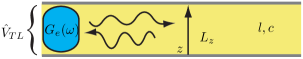
Figure 1: (Color online) Metallic island (blue) coupled to the electromagnetic field of a transmission line (lines around the yellow region). The voltage between the strips is $\hat{V}_{\mathrm{TL}}$.

The studied model consists of a small metallic island coupled to a parallel strip transmission line, see Fig. 1. The transmission line acts as a waveguide supporting a one-dimensional electromagnetic field. In contrast to three-dimensional waveguides, the parallel strip line field has only one allowed field polarization. Therefore it corresponds to a single transport channel. There is no direct electrical connection between the electrons on the island and those in the transmission line strips, only the field couples to the electrons. The total Hamiltonian of the system is $H=H_{\mathrm{e}}+H_{\gamma}+H_{\mathrm{e-\gamma}}$, where

$$H_{\mathrm{e}}= \int\hat{\Psi}^{\dagger}(r)\left(\frac{\hat{p}^{2}}{2m}+U(r)\right)\hat{\Psi}(r)dr+$$

$$+\frac{1}{2}\int\hat{\Psi}^{\dagger}(r)\hat{\Psi}^{\dagger}(r^{\prime})V(r,r^{\prime})\hat{\Psi}(r^{\prime})\hat{\Psi}(r)drdr^{\prime},$$ (1)

$$H_{\gamma}= \sum_{j}\hbar\omega_{j}(\hat{a}_{j}^{\dagger}\hat{a}_{j}+\frac{1}{2})$$ (2)

$$H_{\mathrm{e-\gamma}} =g\int\hat{\Psi}^{\dagger}(r)z\hat{\Psi}(r)dr\hat{V}_{\mathrm{TL}}.$$ (3)

In the following, we do not have to specify the terms in the electron Hamiltonian $H_{e}$ in more detail. The transmission line is characterized by its length $L$, distance between the parallel strips $L_{z}$, and inductance $l$ and capacitance $c$ per unit length. Operator $\hat{V}_{\mathrm{TL}}=\sum_{j}T_{j}(\hat{a}_{j}+\hat{a}_{j}^{\dagger})$ is the voltage operator at the end of the line. The integration in $H_{\mathrm{e-\gamma}}$ is restricted to the region between the parallel strips in the case the electron system extends beyond that. The island is assumed to be much smaller than the photon wavelength at the relevant frequencies, so the position dependence of the voltage operator in the interaction term can be neglected. The field operators $\hat{\Psi}(r),\hat{\Psi}^{\dagger}(r)$ and creation and annihilation operators $\hat{a}_{j},\hat{a}_{j}^{\dagger}$ satisfy canonical fermion and boson commutation relations. Constants $\omega_{j}=j\pi v/L$ ($j$ is a positive integer), $T_{j}=\sqrt{\hbar\omega_{j}/Lc}$ and $g=e/L_{z}$ can be found by quantizing the line field.blais The wave velocity $v$ in the transmission line is given by $v=1/\sqrt{lc}$.

The electron Hamiltonian $H_{\mathrm{e}}$ does not commute with the total Hamiltonian $H$, thus there is an energy flow between the island and the field. This energy flow into the island is characterized by a current $J_{Q}$ defined as

$$J_{Q}\equiv\langle\dot{H}_{\mathrm{e}}\rangle=-\frac{g}{m}\left\langle\int\hat{\Psi}^{\dagger}(r)\hat{p}_{z}\hat{\Psi}(r)dr\hat{V}_{\mathrm{TL}}\right\rangle.$$ (4)

The notation $\langle\cdot\rangle$ stands for averaging over a density matrix of the total system. We calculate averages over nonequilibrium states where subsystems have a temperature gradient or electron system is subjected to a finite voltage. To simplify expressions, the following shorthand notations are introduced: $\hat{P}=\int\hat{\Psi}^{\dagger}(r)\hat{p}_{z}\hat{\Psi}(r)dr$, $\hat{Z}=\int\hat{\Psi}^{\dagger}(r)z\hat{\Psi}(r)dr$ and $\hat{I}=\frac{e}{mL_{z}}\hat{P}$. The quantities are related by $\dot{\hat{Z}}=\hat{P}/m$. The current (4) can be written as

$$J_{Q}(t)= -\frac{2g}{m}\mathrm{Re}\sum_{j}T_{j}G_{j}^{<}(t,t),$$ (5)

$$G_{j}^{<}(t,t^{\prime})\equiv \langle\hat{P}(t)\hat{a}_{j}(t^{\prime})\rangle.$$

The energy transport problem is reduced to finding the ”lesser” Green’s function $G_{j}^{<}(t,t^{\prime})$. We will concentrate on a steady-state situation where $G_{j}^{<}(t,t^{\prime})=G_{j}^{<}(t-t^{\prime})$.

The contour-ordered Green’s function $G_{j}(\tau,\tau^{\prime})$ can be derived by the equation-of-motion technique.haug Let us first consider the time-ordered Green’s function $G_{j}^{t}(t-t^{\prime})$ at $T=0$. By differentiation and applying Heisenberg’s equation of motion we obtain

$$(i\partial_{t^{\prime}}-\omega_{j})G_{j}^{t}(t-t^{\prime})=\frac{g}{\hbar}T_{j}\langle\hat{P}(t)\hat{Z}(t^{\prime})\rangle^{t}.$$ (6)

The expression in brackets on the left hand side of Eq. (6) can be interpreted as an inverse Green’s function $D_{j}^{t\,-1}$ of a free photon field. Thus Eq. (6) can be solved by integration, yielding

$$G_{j}^{t}(t-t^{\prime})=\frac{g}{\hbar}T_{j}\int dt_{1}\langle\hat{P}(t)\hat{Z}(t_{1})\rangle^{t}D_{j}^{t}(t_{1}-t^{\prime}).$$

Using analytical continuation rules known as the Langreth’s theorem,haug we obtain

$$G_{j}^{<}(t-t^{\prime})=\frac{g}{\hbar}T_{j} \int dt_{1}\left[\langle\hat{P}(t)\hat{Z}(t_{1})\rangle^{r}D_{j}^{<}(t_{1}-t^{\prime})+\right.$$

$$\left.+\langle\hat{P}(t)\hat{Z}(t_{1})\rangle^{<}D_{j}^{a}(t_{1}-t^{\prime})\right].$$

Superscripts ^r, ^a and ^< stand for ”retarded”, ”advanced” and ”lesser”. For later purposes it is convenient to define the Fourier transform

$$G_{j}^{<}(\omega)=\frac{1}{\hbar}g\,T_{j}\left[\langle\hat{P}\hat{Z}\rangle^{r}(\omega)D_{j}^{<}(\omega)+\langle\hat{P}\hat{Z}\rangle^{<}(\omega)D_{j}^{a}(\omega)\right]=$$

$$-\frac{gL_{z}^{2}\,m}{\hbar e^{2}}T_{j}\left[\frac{i}{\omega}\langle\hat{I}\hat{I}\rangle^{r}(\omega)D_{j}^{<}(\omega)+\frac{i}{\omega}\langle\hat{I}\hat{I}\rangle^{<}(\omega)D_{j}^{a}(\omega)\right].$$

Now Eq. (5) yields for the steady-state current

$$J_{Q}= \frac{2}{\hbar}\mathrm{Re}\sum_{j}T_{j}^{2}\int_{-\infty}^{\infty}\frac{d\omega}{2\pi}\times$$

$$\times \left[\frac{i\langle\hat{I}\hat{I}\rangle^{r}(\omega)}{\omega}D_{j}^{<}(\omega)+\frac{i\langle\hat{I}\hat{I}\rangle^{<}(\omega)}{\omega}D_{j}^{a}(\omega)\right].$$ (7)

For a transmission line much longer than $\hbar\pi v/(k_{B}T)$, the sum over the field modes can be replaced by integration according to $\sum_{j}=\frac{L}{\pi}\int_{0}^{\infty}dk=\frac{L}{\pi v}\int_{0}^{\infty}dw$. The current takes the form

$$J_{Q}= \frac{2Z_{0}}{\pi}\mathrm{Re}\int d\omega_{j}\hbar\omega_{j}\int\frac{d\omega}{2\pi}\times$$

$$\times\left[\frac{i\langle\hat{I}\hat{I}\rangle^{r}(\omega)}{\hbar\omega}D_{j}^{<}(\omega)+\frac{i\langle\hat{I}\hat{I}\rangle^{<}(\omega)}{\hbar\omega}D_{j}^{a}(\omega)\right],$$ (8)

where $Z_{0}=\sqrt{l/c}$ is the characteristic impedance of the transmission line.

The photon Green’s functions at a finite temperature can be written as $D_{j}^{<}=-2\pi in_{\gamma}(\omega)\delta(\omega-\omega_{j})$ and $D_{j}^{a}=\frac{1}{\omega-\omega_{j}-i\eta}=\pi i\delta(\omega-\omega_{j})+P\frac{1}{\omega-\omega_{j}}$, where $n_{\gamma}(\omega)$ is the Bose distribution. Inserting these expressions into Eq. (Photon heat transport in low-dimensional nanostructures) gives

$$\!J_{Q}=2Z_{0}\int_{0}^{\infty}\frac{d\omega}{2\pi}\left[2\mathrm{Re}\langle\hat{I}\hat{I}\rangle^{r}(\omega)n_{\gamma}(\omega)-\langle\hat{I}\hat{I}\rangle^{<}(\omega)\right].$$ (9)

The correlators on the right hand side of Eq. (9) can be expressed in terms of the noise power $S_{I}=\int_{-\infty}^{\infty}e^{i\omega t}\langle\hat{I}(t)\hat{I}(0)\rangle dt$ as $\langle\hat{I}\hat{I}\rangle^{<}(\omega)=S_{I}(-\omega)$ and $\mathrm{Re}\langle\hat{I}\hat{I}\rangle^{r}(\omega)=\frac{1}{2}(S_{I}(\omega)-S_{I}(-\omega))$. Expression (9) is an exact formula for the energy flow and valid even when the electron system is out of equilibrium. However, it contains the exact current-current correlation functions of the metallic island in the presence of the field. In equilibrium, these are related to conductance through the Fluctuation-Dissipation theorem and the Kubo formula. From formal point of view, the exact expression for noise power determines the energy exchange process completely. In the weak-coupling limit (the lowest order in electron-photon coupling), one can neglect the field and use the bare island correlators. On physical grounds one expects that the maximum energy transport is achieved when the coupling is strong, thus a more accurate treatment of the electron-photon interaction is desirable.

The quadratic form of $H_{\gamma}$ and the linear coupling term $H_{\mathrm{e-ph}}$, together with the density of states of a long transmission line is precisely a Caldeira-Leggett representation of an ohmic loss.legget Solution to the equation of motion of the voltage operator is $\hat{V}_{\mathrm{TL}}(t)=\hat{V}_{\mathrm{TL}}^{0}(t)+Z_{0}\hat{I}(t)$, where $\hat{V}_{\mathrm{TL}}^{0}(t)$ is the solution in the absence of the island and $\hat{I}(t)$ is the current flowing in the electron system. This notion microscopically motivates the circuit approximation, where the transmission line can be thought as a resistor in series with the metallic island, see Fig. 2 a).

In the circuit description correlation functions can be calculated by the Langevin approach, which allows us to relate the current fluctuations in the presence of the environment to bare quantities.blanter This yields

$$\langle\hat{I}\hat{I}\rangle(\omega)=\frac{\langle\hat{I}\hat{I}\rangle_{e}(\omega)}{|1+G_{e}(\omega)Z_{0}|^{2}},$$ (10)

where $\langle\hat{I}\hat{I}\rangle_{e}(\omega)$ and $G_{e}(\omega)$ are the current-current correlation function and conductance of the island in the absence of the electromagnetic field. According to the Kubo formula for conductance, the real part of the retarded function appearing in Eq. (9) is related to the conductance as $\mathrm{Re}[G_{e}(\omega)]=\mathrm{Re}[\langle\hat{I}\hat{I}\rangle_{e}^{r}(\omega)]/(\hbar\omega)$. With approximation (10), we then get

$$J_{Q}= \int_{0}^{\infty}\frac{d\omega}{2\pi}\frac{2Z_{0}}{|1+G_{e}(\omega)Z_{0}|^{2}}\times$$

$$\times\left\{[S_{I}^{e}(\omega)-S_{I}^{e}(-\omega)]n_{\gamma}(\omega)-S_{I}^{e}(-\omega)\right\},$$ (11)

where $S_{I}^{e}(\omega)$ is the noise power for the isolated electron system.

In (quasi)equilibrium the correlation functions are related through a variant of Fluctuation-Dissipation formula $S_{I}^{e}(\omega)=2\mathrm{Re}[G_{e}(\omega)]\hbar\omega n_{e}(\omega)$, where $n_{\mathrm{e}}(\omega)$ is the Bose distribution function at the electron temperature. Thus for this case

$$J_{Q}=\frac{4Z_{0}R_{\mathrm{e}}}{(R_{\mathrm{e}}+Z_{0})^{2}}\int_{0}^{\infty}\frac{d\omega\hbar\omega}{2\pi}\left[n_{\gamma}(\omega)-n_{\mathrm{e}}(\omega)\right],$$ (12)

when the island is assumed resistive $R_{\mathrm{e}}\equiv 1/G_{e}$. Result (12) agrees with the one stated in Ref. schmidt, for heat flow between two resistors. After integration Eq. (12) gives

$$J_{Q}=r\frac{\pi^{2}k_{B}^{2}}{6h}(T_{\gamma}^{2}-T_{\mathrm{e}}^{2}),\quad r\equiv\frac{4Z_{0}R_{\mathrm{e}}}{(R_{\mathrm{e}}+Z_{0})^{2}}$$ (13)

At small temperature difference this is just

$$J_{Q}=rG_{Q}\Delta T,$$ (14)

where $G_{Q}=\pi^{2}k_{B}^{2}T/3h$ is the universal quantum of heat conductance pendry . Thus, when $R_{e}=Z_{0}$ and thus $r=1$, the maximum one-channel heat transfer is achieved. In the weak-coupling limit, where the exact correlation functions in (9) are replaced by bare correlators $\langle\hat{I}\hat{I}\rangle_{0}(\omega)$, one recovers (14) with the prefactor $Z_{0}R_{\mathrm{e}}/(R_{\mathrm{e}}+Z_{0})^{2}$ replaced by $Z_{0}/R_{\mathrm{e}}$. Physically the weak coupling result follows from the impedance mismatch $Z_{0}\ll R_{\mathrm{e}}$.

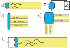
Figure 2: (Color online) a) Circuit picture corresponding to the studied system. Transmission line acts as a series resistor to the island. In b) the parallel transmission lines couple to vertical current noise and in c) the lines couple to vertical and horizontal noise. The maximum heat conductance in b) is $G_{Q}$ and in c) is $2G_{Q}$. The number of parallel transmission lines is irrelevant for the maximum heat conductance. In d) the island contains a short conductor and is externally biased.

The above discussion can be generalized to incorporate several photon channels realized by coupling the electron system to, say, $N$ transmission lines, as in Fig. 2. Suppose that each transmission line is described by a Hamiltonian of the form (2) with the coupling (3) corresponding to the situation in Fig. 2 b). The theoretical maximum heat conductance for $N$ independent channels is $N\times G_{Q}$, but it is not achieved in this case. An added transmission line does not simply add an independent photon channel because it also effectively acts as a series resistor in the coupling direction. Thus it suppresses current fluctuations and affects the emitted energy in all channels. The heat flow (14) for multiple channels is

$$J_{Q}=\sum_{i}G_{Q}^{i}\frac{4R_{i}Z_{i}}{(R_{i}+\sum_{i}Z_{i})^{2}}\Delta T_{i},$$ (15)

where $Z_{i}$ is the characteristic impedance, $\Delta T_{i}$ the temperature difference and $R_{i}$ the electron resistance associated with line $i$. When all the transmission line fields are at the same temperature, the maximum heat conductance given by Eq. (15) is still $G_{Q}$. Thus, adding parallel lines does not increase this maximum. However, coupling the island to perpendicular transmission lines, as in Fig. 2 c), opens up an independent transport channel. The difference in b) and c) is that the lines in perpendicular directions couple to different current components. The flow $J_{Q}$ is then a sum of two terms of the form (15) and the maximum heat conductance is $2G_{Q}$. Similarly, coupling to the remaining orthogonal direction yields the maximum heat conductance 3$G_{Q}$.

Next we consider a case where the island contains a short contact which is externally biased by potential difference, see Fig. 2 d). Supposing that the electron transport is coherent and neglecting interaction effects, current noise contains both the equilibrium and shot noise and can be written as aguado

$$\begin{split}S_{I}(\omega)&=G_{0}\sum_{m}T_{m}(1-T_{m})\bigg{[}\frac{eV+\hbar\omega}{1-e^{\beta(-\hbar\omega-eV)}}\\ &+\frac{-eV+\hbar\omega}{1-e^{\beta(-\hbar\omega+eV)}}\bigg{]}+G_{0}\sum_{m}T_{m}^{2}\frac{2\hbar\omega}{1-e^{-\beta\hbar\omega}},\end{split}$$ (16)

where $G_{0}=e^{2}/h$, $V$ is the bias voltage and $T_{m}$ is the transmission eigenvalue of channel $m$. The sums of transmission eigenvalues extend over the channel index and the spin. Inserting expression (16) to the general formula (9) we discover

$$J_{Q}^{\gamma}=r\left[\frac{1}{2}G_{0}\mathcal{L}_{0}(T_{\gamma}^{2}-T_{\mathrm{e}}^{2})-\frac{1}{2}F_{2}GV^{2}\right],$$ (17)

where $G=G_{0}\sum_{m}T_{m}=1/R_{e}$ is the island conductance, $F_{2}=\sum_{m}T_{m}(1-T_{m})/\sum_{m}T_{m}$ the Fano factor, and $\mathcal{L}_{0}=\pi^{2}k_{\mathrm{B}}^{2}/3e^{2}$ the Lorenz number. The last term in $J_{Q}^{\gamma}$ corresponds to the increased emission by shot noise. The frequency dependence in Eq. (16) is solely due to the Fermi distribution and the emitted energy due to shot noise shows only dependence on the bias voltage. Expression (16) is valid only for low frequencies; generally $S_{I}(\omega)$ probes the intrinsic (inverse) time scales of the conductor such as the time of flight and the charge relaxation time. This is shown in Fig. 3 where we have used the noise and conductance of an interacting chaotic cavity hekking to numerically compute the energy flow.

Assume that the island is biased using superconducting wires with contact conductances much higher than $G$. Such a setup provides thermal insulation of the island meschke while the voltage still drops across the contact. The final temperature $T_{e}$ of the island can be obtained from a heat balance equation where the Joule heating $J_{Q}^{J}$ from the voltage source is balanced by heat flow to photons and phonons as $J_{Q}^{J}+J_{Q}^{\gamma}+J_{Q}^{\mathrm{ph}}=GV^{2}+J_{Q}^{\gamma}+\Sigma\Omega[T_{\mathrm{ph}}^{5}-T_{e}^{5}]=0,$ where $\Sigma$ is the electron-phonon coupling constant giazotto and $\Omega$ is the volume of the island. There is a crossover temperature $T_{\rm cr}=(rG_{0}\mathcal{L}_{0}/(2\Sigma\Omega))^{1/3}$ below which the photon transport is the dominant process. For example, with the parameters of Ref. meschke, , $T_{\rm cr}$ would be roughly 140 mK – for smaller objects such as carbon nanotubes, it could be made larger at least by one order of magnitude. Much below $T_{\rm cr}$ the final electron temperature is

$$T_{e}=\sqrt{T_{\gamma}^{2}+\frac{T_{\rm ph}^{5}}{T_{\rm cr}^{3}}+\frac{2G}{G_{0}r}\left(1-\frac{F_{2}r}{2}\right)\frac{V^{2}}{\mathcal{L}_{0}}}$$ (18)

and above the crossover it is

$$T_{e}=\left(T_{\mathrm{ph}}^{5}+T_{\rm cr}^{3}T_{\gamma}^{2}+G\left(1-\frac{F_{2}r}{2}\right)\frac{V^{2}}{\Sigma\Omega}\right)^{\frac{1}{5}}.$$ (19)

In both limits the Joule heating is reduced by the factor $(1-F_{2}r/2)$ because a fraction of it flows to photons. In the case of an ideally matched ($r=1$) tunnel junction ($F_{2}=1$), exactly half of the Joule heat goes to photons. In experiments the parameters $V$, $T_{\rm ph}$, $T_{\gamma}$ and $r$ can be varied in situ to investigate the photon transport contribution, as demonstrated in Ref. meschke, for $r$, $T_{\rm ph}$ and $T_{\gamma}$.

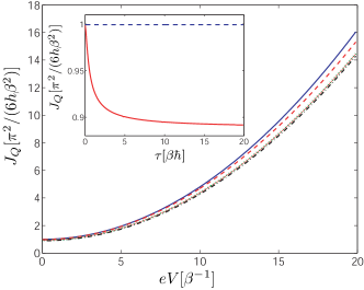
Figure 3: (Color online) Energy flow from a symmetric chaotic cavity $(N_{L}=N_{R}=1)$ as a function of voltage. We assumed that the cavity conductance at zero frequency $G_{e}(0)$ is matched to $Z_{0}^{-1}$. The different curves correspond to different cavity charge relaxation times $\tau$, $\tau=0$ (solid), $\tau=0.1\hbar\beta$ (dashed), $\tau=\hbar\beta$ (dotted), $\tau=10\hbar\beta$ (dash-dotted). Inset shows the $\tau/\hbar\beta$-dependence of the heat flow from the cavity ($V=0$), the horizontal dashed line corresponds to the heat flow from an ideally matched ohmic resistor without frequency dependence. When $\tau/\hbar\beta\ll 1$ the heat flow is close to the theoretical maximum and settles to a lower value as the fraction increases.

In conclusion, we studied a microscopic model of photon transport in nanostructures using a Green’s-function method and derived a general expression for the energy flow between a metallic island and a transmission line field. We showed how electron and photon transport are related through frequency-dependent current noise. We demonstrated efficiency of the energy flow formula by deriving quantized photon heat conductance and studying effects of electron shot noise to photon transport. We propose to measure the shot-noise effect illustrated as the voltage-dependent term in Eq. (17) by modifying the setup in Ref. meschke, to include a small mesoscopic junction.

We thank Jukka Pekola, Matthias Meschke and Henning Schomerus for insightful discussions. TTH acknowledges the Academy of Finland for funding.

References

(1)J. B. Pendry, J. Phys. A: Math. Gen. 16, 2161 (1983).
(2) L. G. C. Rego, G. Kirczenow, Phys. Rev. B 59, 13080
(1999); M. P. Blencowe, V. Vitelli, Phys. Rev. A 62, 052104
(2000).
(3) O. Chiatti, et al., Phys. Rev. Lett. 97, 056601 (2006).
(4) K. Schwab, E. A. Henriksen, J. M. Worlock and M. L. Roukes, Nature 404, 974 (2000).
(5) M. Meschke, W. Guichard and J. P. Pekola, Nature 444, 187 (2006).
(6)D. R. Schmidt, R. J. Schoelkopf and A. N. Cleland, Phys. Rev. Lett. 93, 045901 (2004).
(7) F. Giazotto, et al., Rev. Mod. Phys. 78, 217 (2006).
(8)A. Wallraff, et al., Nature 431, 162 (2004).
(9)A. Blais, R.-S. Huang, A. Wallraff, S. M. Girvin and R. J. Schoelkopf, Phys. Rev. A 69, 062320 (2004).
(10) H. Haug, A.-P. Jauho, Quantum Kinetics in Transport and Optics of Semiconductors (Springer-Verlag, Berlin Heidelberg, 1996).
(11)A. J. Leggett, et al., Rev. Mod. Phys. 59, 1 (1987).
(12) Ya. M. Blanter, M. Büttiker, Phys. Rep. 336, 1 (2000).
(13)R. Aguado, L. P. Kouwenhoven, Phys. Rev. Lett. 84, 1986 (2000).
(14) F. W. J. Hekking and J. P. Pekola, Phys. Rev. Lett. 96, 056603
(2006); P. W. Brouwer and M. Büttiker, Europhys. Lett. 37,
441 (1996).