Rapidly rotating boson molecules with long or short range repulsion:
an exact diagonalization study

Abstract

The Hamiltonian for a small number, $N\leq 11$, of bosons in a rapidly rotating harmonic trap, interacting via a short range (contact potential) or a long range (Coulomb) interaction, is studied via an exact diagonalization in the lowest Landau level. Our analysis shows that, for both low and high fractional fillings, the bosons localize and form rotating boson molecules (RBMs) consisting of concentric polygonal rings. Focusing on systems with the number of trapped atoms sufficiently large to form multi-ring bosonic molecules, we find that, as a function of the rotational frequency and regardless of the type of repulsive interaction, the ground-state angular momenta grow in specific steps that coincide with the number of localized bosons on each concentric ring. Comparison of the conditional probability distributions (CPDs) for both interactions suggests that the degree of crystalline correlations appears to depend more on the fractional filling $\nu$ than on the range of the interaction. The RBMs behave as nonrigid rotors, i.e., the concentric rings rotate independently of each other. At filling fractions $\nu<1/2$, we observe well developed crystallinity in the CPDs (two-point correlation functions). For larger filling fractions $\nu>1/2$, observation of similar molecular patterns requires consideration of even higher-order correlation functions.

I Introduction

Rotating ultra-cold trapped Bose condensed systems are most commonly discussed in the context of formation of vortex lattices, which are solutions to the Gross-Pitaevskii (GP) mean-field equation stri ; legg ; ho ; fett ; peth ; pita ; baks1 ; baks2 ; peth2 ; baym1 . Such vortex lattices have indeed been found experimentally for systems containing a large number of bosons dali ; kett ; corn . Nevertheless, several theoretical investigations wilk1 ; vief ; wilk2 ; regn1 ; regn2 of rapidly rotating trapped bosonic systems suggested formation of strongly correlated exotic states which differ drastically from the aforementioned vortex-lattice states. While experimental realizations of such strongly correlated states have not been reported yet, there is already a significant effort associated with two-dimenional (2D) exact-diagonalization (EXD) studies of a small number of particles ($N$) in the lowest Landau level, LLL; the LLL restriction corresponds to the regime of rapid rotation, where the rotational frequency of the trap $\Omega$ equals the frequency $\omega_{0}$ of the confining potential. The large majority wilk1 ; wilk2 ; regn1 ; regn2 of such EXD studies have attempted to establish a close connection between rapidly rotating bosonic gases and the physics of elecrtons under fractional-quantum-Hall-effect (FQHE) conditions employing the bosonic version of “quantum-liquid” analytic wave functions, such as the Laughlin wave functions, composite-fermion, Moore-Read, and Pfaffian functions.

Recently, the “quantum-liquid” picture for a small number of trapped electrons in the FQHE regime has been challenged in a series of extensive studies yl1 ; yl2 ; yl3 ; yl4 ; yl5 ; yl6 of electrons in 2D quantum dots under high magnetic fields ($B$). Such studies (both EXD and variational) revealed that, at least for finite systems, the underlying physical picture governing the behavior of strongly-correlated electrons is not that of a “quantum liquid.” Instead, the appropriate description is in terms of a “quantum crystal,” with the localized electrons arranged in polygonal concentric rings yl1 ; yl2 ; yl3 ; yl4 ; yl5 ; bao ; seki ; maks . These “crystalline” states lack yl3 ; yl5 the familiar rigidity of a classical extended crystal, and are better described yl1 ; yl2 ; yl3 ; yl4 ; yl5 ; yl6 as rotating electron (or Wigner) molecules (REMs or RWMs).

Motivated by the discovery in the case of electrons of REMs at high $B$ (and from the fact that Wigner molecules form also at zero magnetic field yl7 ; egge ; yl8 ; mikh ; yl9 ; yl10 ) some theoretical studies have most recently shown that analogous molecular patterns of localized bosons do form in the case of a small number of particles inside a static or rotating harmonic trap yl11 ; yl12 ; yl13 ; mann ; barb . In analogy with the electron case, the bosonic molecular structures can be referred to yl13 as rotating boson molecules (RBMs); a description of RBMs via a variational wave function note1 built from symmetry-breaking displaced Gaussian orbitals with subsequent restoration of the rotational symmetry was presented in Refs. yl11 ; yl12 ; yl13 .

In this paper, we use exact diagonalization in the lowest Landau level to investigate the formation and properties of RBMs focusing on a larger number of particles than previously studied, in particular for sizes where multiple-ring formation can be expected based on our knowledge of the case of 2D electrons in high $B$. We study a finite number of particles ($N\leq 11$) at both low ($\nu<1/2$) and high ($\nu\geq 1/2$) filling fractions $\nu\equiv N(N-1)/2L$ note56 (where $L\equiv{\cal L}/\hbar$ is the quantum number associated with the total angular momentum ${\cal L}$) and investigate both the cases of a long (Coulomb) and a short ($\delta$-function) range repulsive interaction.

As in the case of electrons in 2D quantum dots, we probe the crystalline nature of the bosonic ground states by calculating the full anisotropic two-point correlation function $P({\bf r},{\bf r}_{0})$ associated with the exact wavefunction $\Psi({\bf r}_{1},{\bf r}_{2},...,{\bf r}_{N})$. The quantity $P({\bf r},{\bf r}_{0})$ is proportional to the probability of finding a boson at ${\bf r}$ given that there is another boson at the observation point ${\bf r}_{0}$, and it is often referred to as the conditional probability distribution yl4 ; yl5 ; yl8 ; yl10 ; yl11 ; yl13 (CPD). A main finding of our study is that consideration solely of the CPDs is not sufficient for the boson case at high fractional fillings $\nu\geq 1/2$; in this case, one needs to calculate even higher-order correlation functions, e.g., the full $N$-point correlation function $P({\bf r};{\bf r}_{1},{\bf r}_{2},...,{\bf r}_{N-1})$ [see Eq. (12)].

The present investigations are also motivated by recent experimental developments, e.g., the emergence of trapped ultra-cold gas assemblies featuring bosons interacting via a long-range dipole-dipole interaction. We expect the results of this paper to be directly relevant to such systems with a two-body repulsion intermediate between the Coulomb and the delta potentials. Additionally, we note the appearance of promising experimental techniques for measuring higher-order correlations in ultra-cold gases employing an atomic Hanbury Brown-Twiss scheme orsay or shot-noise interferometry shot_noise_1 ; shot_noise_2 . Experimental realization of few-boson rotating systems can be anticipated in the near future as a result of increasing sophistication of experiments involving periodic optical lattices co-rotating with the gas, which are capable of holding a few atoms in each site. A natural first step in the study of such systems is the analysis of the physical properties of a few particles confined in a rotating trap with open boundary conditions (i.e., conservation of the total angular momentum $L$), such as we do here.

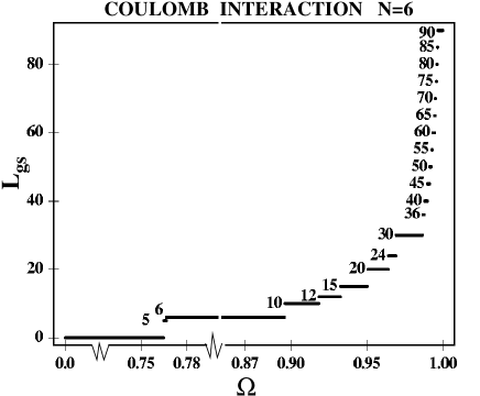
Figure 1: Ground-state angular momenta, $L_{\text{gs}}$, for $N=6$ bosons in a rapidly rotating trap [described by the LLL Hamiltonian in Eq. (3)], as a function of the rotational frequency $\Omega$ expressed in units of $\omega_{\bot}$. The bosons interact via a Coulombic repulsion and the many-body Hilbert space is restricted to the LLL. The angular momentum associated with the first bosonic Laughlin state occurs at $L=30$, i.e., at $N(N-1)$. The value of $c=0.2\hbar\omega_{\bot}\Lambda$ for this plot; the many-body wave function does not depend on this choice. Note the stepwise variation of the values of the ground-state angular momenta, indicating the presence of an intrinsic point-group symmetry associated with the polygonal-ring structure of RBMs (see text for details).

Our main results can be summarized as follows: Similar to the well-established (see, e.g., Refs. yl4 ; yl5 ) formation of rotating electron molecules in quantum dots, we describe here the emergence of rotating boson molecules in rotating traps. The RBMs are also organized in concentric polygonal rings that rotate independently of each other, and the polygonal rings correspond to classical equilibrium configurations and/or their low-energy isomers. Furthermore, the degree of crystallinity increases gradually with larger angular momenta $L$’s (smaller filling fractions $\nu$’s), as was the trend yl2 ; yl4 ; yl5 for the REMs and as was observed also for $\nu<1/2$ in another study mann for rotating bosons in the LLL with smaller $N$ and single-ring structures. We finally note that the crystalline character of the RBMs appears to depend only weakly on the range of the repelling interaction, for both the low (see also Ref. mann ) and high (unlike Ref. barb ) fractional fillings note2 .

In studies of 2D quantum dots, CPDs were used some time ago in Refs. seki ; maks ; yl8 ; note67 . For probing the intrinsic molecular structure in the case of ultracold bosons in 2D traps, however, they were introduced only recently by Romanovsky et al. yl11 . The importance of using CPDs as a probe can hardly be underestimated. Indeed, while EXD calculations for bosons in the LLL have been reported earlier wilk1 ; vief ; wilk2 ; regn1 ; regn2 , the analysis in these studies did not include calculations of the CPDs, and consequently formation of rotating boson molecules was not recognized.

This paper is organized as follows. In section II we establish our notation and detail the physical assumptions that underlie the construction of our ab initio Hamiltonian. In section III, we present our results for $N=6,9$ and 11 bosons and compare the emerging crystallinity for both Coulomb and $\delta$-function interactions. We summarize our results in section IV. The appendix presents explicit formulas for calculations of two-body matrix elements between two permanents. These permanents are used as the basis wave functions that span the many-boson Hilbert space; for the case of fermions, of course, one uses the more familiar Slater determinants yl2 .

Figure 2: Ground-state angular momenta, $L_{\text{gs}}$, for $N=6$ bosons in a rapidly rotating trap [described by the LLL Hamiltonian in Eq. (3)], as a function of the rotational frequency $\Omega$ expressed in units of $\omega_{\bot}$. The bosons interact via a delta repulsion and the many-body Hilbert space is restricted to the LLL. The angular momentum associated with the first bosonic Laughlin state occurs at $L=30$, i.e., at $N(N-1)$. The value of $g=2\pi\hbar\omega_{\bot}\Lambda^{2}/N$ for this plot; the many-body wave function does not depend on this choice. The values of the angular momenta terminate with the value $L=30$ (the Laughlin value) at $\Omega/\omega_{\bot}=1$. In contrast, in the Coulomb-interaction case (see Fig. 1), the values of the ground-state angular momenta do not terminate, but diverge as $\Omega/\omega_{\bot}\rightarrow 1$. Note the stepwise variation of the values of the ground-state angular momenta in both cases, indicating the presence of an intrinsic point-group symmetry associated with the polygonal-ring structure of RBMs (see text for details).

II Theoretical methods

II.1 Ab initio Hamiltonian in the LLL

Requiring a very strong confinement of the harmonic trap along the axis of rotation ($\hbar\omega_{z}>>\hbar\omega_{\bot}$), freezes out the many body dynamics in the $z$-dimension, and the wavefunction along this direction can be assumed to be permanently in the corresponding oscillator ground state. We are thus left with an effectively 2D system. For such a setup, the Hamiltonian for $N$ atoms of mass $m$ in a harmonic trap $(\omega_{\bot})$ rotating at angular frequency $\Omega\hat{\bf z}$ is given by:

$$H=\sum_{i=1}^{N}\left(\frac{{\bf p}_{i}^{2}}{2m}+\frac{1}{2}m\omega_{\bot}^{2}{\bf r}_{i}^{2}\right)+\sum_{i<j}^{N}v({\bf r}_{i}-{\bf r}_{j})-\Omega{\cal L}.$$ (1)

Here ${\cal L}=-\hbar L=\sum_{i=1}^{N}\hat{{\bf z}}\!\cdot{\bf r}_{i}\times{\bf p}_{i}$ is the total angular momentum; ${\bf r}\;=\;(x,y)$ and ${\bf p}\;=(p_{x},p_{y})$ represent the single-particle position and angular momentum in the $x-y$ plane and $\omega_{\bot}$ is the radial trap frequency.

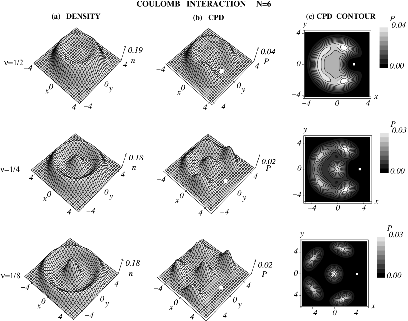
Figure 3: (a) Single-particle densities [$n({\bf r})$; left column], (b) CPDs $\left[P({\bf r},{\bf r}_{0})\right]$ in 3D plots (middle column), and (c) CPDs in contour plots (right column), portraying the strengthening of the crystalline RBM structure for $N=6$ bosons interacting via a repulsive Coulomb interaction as the filling fraction $\nu$ is reduced. The white dots in the CPD plots indicate the reference point ${\bf r}_{0}$. We note in particular the gradual enhancement of the peak at the center of the plots, and the growth of the radius of the outer ring; the latter reflects the nonrigid-rotor nature of the RBMs (in analogy with the findings of Ref. yl5 regarding the properties of rotating electron molecules). The cases of $\nu=1/4$ and $\nu=1/8$ exhibit a clear $(1,5)$ crystalline arrangement, while the case of $\nu=1/2$ (first Laughlin state) is intermediate between a $(1,5)$ and a $(0,6)$ pattern (see text for details). Lengths in units of $\Lambda$. The vertical scales are in arbitrary units, which however do not change for the panels within the same column (a), (b), or (c).

The Hamiltonian can be rewritten in the form,

$$H = \sum_{i=1}^{N}\left\{\frac{\left({\bf p}_{i}-m\Omega\hat{\bf z}\times{\bf r}_{i}\right)^{2}}{2m}+\frac{m}{2}(\omega_{\bot}^{2}-\Omega^{2}){\bf r}_{i}^{2}\right\}$$ (2)

$$~{}~{}~{}~{}~{}~{}~{}~{}~{}~{}~{}+\sum_{i<j}^{N}v({\bf r}_{i}-{\bf r}_{j}).$$

The kinetic part of this Hamiltonian is formally equivalent to that of the Hamiltonian in the symmetric gauge of an electron (of charge $e$ and mass $m_{e}$) moving in two dimensions under a constant perpendicular magnetic field $B$, if one makes the identification that the cyclotron frequency $\omega_{c}=eB/(m_{e}c)\rightarrow 2\Omega$.

We are now ready to examine our main approximation which is based on two assumptions: (1) that the rotational frequency $\Omega$ is close to that of the confining trap; in this case the external confinement can be neglected in a first approximation and thus the single-particle spectra are organized in infinitely-degenerate Landau levels that are separated by an energy gap of $2\hbar\omega_{\bot}$, and (2) that the interaction strength is so weak that the mixing of Landau levels can be ignored. Since we work at zero temperature it then follows that all particles are in the lowest Landau level. This physical regime is known in the literature as the weak interaction limit. In a recent paper feder it has been verified by explicit calculation that this approximation, i.e., the lowest Landau level approximation, is very good for $\nu<1/2$ (low fractional fillings), where strong crystalline correlations are most developed, as reported in the present work.

We note, however, that strong correlations beyond the Gross-Pitaevskii mean field persist in the LLL even for $\nu>1/2$ (high fractional fillings), as was found via EXD calculations for smaller $N$ in Ref. barb . In particular, Ref. barb concluded that even in the most favorable case (i.e., for $L=N$) formation of vortices for small $N$ is not a prevalent phenomenon, and their appearance “is restricted to the vicinity of some critical values of the rotational frequency $\Omega$.” This conclusion concurs with the results of Ref. yl13 which used RBM variational wave functions to study a broad range of rotational frequencies that do not lead to the restriction to the LLL. The present work brings new insights to these findings by showing that the crystalline correlations for $\nu>1/2$ (high fractional fillings) are clearly seen in the $N$-point correlation functions, even though an inspection of the CPDs alone may be inconclusive (see examples in Section III.A).

Taking into account that the single-particle spectrum associated with the Hamiltonian (2) (Fock-Darwin spectrum fock ; darw ) is given by $\epsilon^{\text{FD}}_{n,l}=\hbar[(2n+|l|+1)\omega_{\bot}-l\Omega]$, the restriction to the LLL requires $n=0$ (Fock-Darwin single-particle states with zero radial nodes) and reduces the Hamiltonian $H$ above [Eq. (2)] to the simpler form:

$$H_{\text{LLL}}=N\hbar\omega_{\bot}+\hbar(\omega_{\bot}-\Omega)L+\sum_{i<j}^{N}v({\bf r}_{i}-{\bf r}_{j}),$$ (3)

for which only the interaction term is non-trivial, since the many-body energy eigenstates are eigenstates of the total angular momentum as well; $L=\sum_{i=1}^{N}l_{i}$.

In this study we shall investigate and compare our results for strongly correlated states in the LLL obtained for a system of bosons interacting via a long or short range force respectively represented by the coulomb interaction,

$$v({\bf r})=\frac{c}{|{\bf r}|},$$ (4)

or the contact potential,

$$v({\bf r})=g\delta^{2}({\bf r}).$$ (5)

As may be inferred from the form of $H_{\text{LLL}}$ the coupling constants $c$ and $g$ trivially change the result by a multiplicative factor and their importance occurs only in comparing our results to a particular experimental system. Mathematically expressed, our description is valid only when:

$$g\Lambda^{-2}\ll 2\hbar\omega_{\bot}\ll\hbar\omega_{z}$$ (6)

in the case of a contact potential, and

$$\frac{c}{\Lambda}\ll 2\hbar\omega_{\bot}\ll\hbar\omega_{z},$$ (7)

for the coulomb interaction, with $\Lambda=\sqrt{\hbar/(m\omega_{\bot})}$ being the characteristic length of the harmonic trap. In these inequalities we have, for the sake of completeness, also included the energy scale associated with the ’frozen’ perpendicular direction to give a full picture of the hierarchy of energy scales implicit in our approximations.

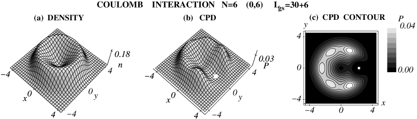
Figure 4: A ground state with a well-developed $(0,6)$ arrangement for $N=6$ bosons interacting via a Coulomb repulsion at angular momentum $L_{\text{gs}}=36$. In classical electrostatic calculations peeters_classical , the $(0,6)$ arrangement is the first metastable isomer to the most stable $(1,5)$ one shown by the CPDs of Fig. 3. The individual panels are: (a) $3D$ plot of the single-particle density $n({\bf r})$; (b) $3D$ plot of the CPD; and (c) Contour plot of the CPD. In the CPD $\left[P({\bf r},{\bf r}_{0})\right]$ plots, the white dots indicate the reference point ${\bf r}_{0}$. Lengths in units of $\Lambda$. In (b) and (c), the vertical scales are the same.

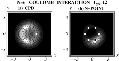
Figure 5: Contour plots of the CPD (a) and $N$-point correlation function (b) for $N=6$ bosons with $L_{\text{gs}}=12$ interacting via a Coulomb repulsion. The white squares indicate the positions of the fixed particles. The black square in (b) indicates the position of the 6th particle according to the classical $(0,6)$ molecular configuration. Note that the CPD in (a) fails to reveal the $(0,6)$ pattern, which, however, is clearly seen in the $N$-point correlation function in (b). Lengths in units of $\Lambda$. The vertical scales are arbitrary.

Figure 6: Contour plots of the CPD (a) and $N$-point correlation function (b) for $N=6$ bosons with $L_{\text{gs}}=12$ interacting via a $\delta$-repulsion. The white squares indicate the positions of the fixed particles. The black square in (b) indicates the position of the 6th particle according to the classical $(0,6)$ molecular configuration. Note that the CPD in (a) fails to reveal the $(0,6)$ pattern, which, however, is clearly seen in the $N$-point correlation function in (b). Lengths in units of $\Lambda$. The vertical scales are arbitrary.

II.2 EXD wave function and Conditional Probability Distribution

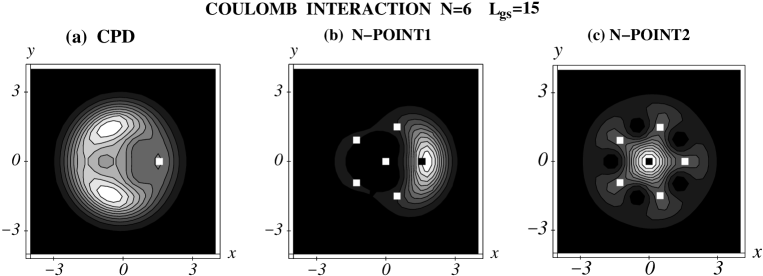
Figure 7: Contour plots of the CPD (a) and $N$-point correlation function (b) and (c) for $N=6$ bosons with $L_{\text{gs}}=15$ interacting via a Coulomb repulsion. The white squares indicate the positions of the fixed particles. The black square in (b) and (c) indicates the position of the 6th particle according to the classical $(1,5)$ molecular configuration. Note the different arrangements of the five fixed particles, i.e., (b) one fixed particle at the center and (c) no fixed particle at the center. Note also that the CPD in (a) fails to reveal the $(1,5)$ pattern, which, however, is clearly seen in the $N$-point correlation functions in both (b) and (c). Lengths in units of $\Lambda$. The vertical scales are arbitrary, but the same in (b) and (c).

For the solution of the large scale, but sparse, matrix eigenvalue problem associated with the Hamiltonina $H_{\text{LLL}}$, we have used the ARPACK computer code arp ; petsc . For a given $L$, the EXD many-body wave function is a linear superposition of permanents made out of the single-particle LLL wave functions,

Figure 8: Contour plots of the CPD (a) and $N$-point correlation function (b) and (c) for $N=6$ bosons with $L_{\text{gs}}=15$ interacting via a $\delta$-repulsion. The white squares indicate the positions of the fixed particles. The black square in (b) and (c) indicates the position of the 6th particle according to the classical $(1,5)$ molecular configuration. Note the different arrangements of the five fixed particles, i.e., (b) one fixed particle at the center and (c) no fixed particle at the center. Note also that the CPD in (a) fails to reveal the $(1,5)$ pattern, which, however, is clearly seen in the $N$-point correlation functions in both (b) and (c). Lengths in units of $\Lambda$. The vertical scales are arbitrary, but the same in (b) and (c).

$$\phi_{l}(z)=\frac{1}{\Lambda\sqrt{\pi l!}}\left(\frac{z}{\Lambda}\right)^{l}e^{-zz^{*}/(2\Lambda^{2})},$$ (8)

with complex coordinates $z=x+iy$. Namely,

$$\Psi(z_{1},z_{2},...,z_{N})=\sum_{J=1}^{K}C_{J}\Phi_{J},$$ (9)

where $\Phi_{J}$ is a normalized permanent (see the Appendix); the index $J$ denotes any set of $N$ single-particle states $\{\phi_{l_{1}}(z_{1}),\phi_{l_{2}}(z_{2}),...,\phi_{l_{N}}(z_{N})\}$ (not necessarily distinct) with angular momenta $\{l_{1},l_{2},...,l_{N}\}$ such that

$$l_{1}\leq l_{2}\leq...\leq l_{N},\;\;\;\;{\text{and}}\;\;\;\;\sum_{k=1}^{N}l_{k}=L.$$ (10)

The dimension $K$ of the Hilbert space is controlled by the maximum allowed single-particle angular momentum $l_{\text{max}}$, such that $l_{k}\leq l_{\text{max}}$, $1\leq k\leq N$. By varying $l_{\text{max}}$, we have checked that this procedure produces well converged numerical results.

We probe the intrinsic structure of the EXD eigenstates [Eq. (9)] for crystalline behavior using the conditional probability distribution $P({\bf r},{\bf r}_{0})$ defined (see, e.g., Ref. yl8 ) by the following expression:

$$P({\bf r},{\bf r}_{0})=\langle\Psi|\sum_{i=1}^{N}\sum_{j\neq i}^{N}\delta({\bf r}_{i}-{\bf r})\delta({\bf r}_{j}-{\bf r}_{0})|\Psi\rangle.$$ (11)

Unlike the case of electrons in QDs yl4 , we found that, for rotating bosons, the CPDs are not sufficient to decipher the intrinsic molecular configuration in the case of high fractional fillings $\nu\geq 1/2$. In such a case, one needs to calculate higher correlation functions. In this paper, we use the $N$-point correlation function defined as the modulus square of the full many-body EXD wave function, i.e.,

$$P({\bf r};{\bf r}_{1},{\bf r}_{2},...,{\bf r}_{N-1})=|\Psi({\bf r};{\bf r}_{1},{\bf r}_{2},...,{\bf r}_{N-1})|^{2},$$ (12)

where one fixes the positions of $N-1$ particles and inquiries about the (conditional) probability of finding the $N$th particle at any position ${\bf r}$.

In the rest of this paper, we often find useful to contrast the CPDs and $N$-point correlations to the single-particle densities $n({\bf r})$, which are circularly symmetric as a result of the total angular momentum being a good quantum number. The single-particle density is defined as

$$n({\bf r})=\langle\Psi|\sum_{i=1}^{N}\delta({\bf r}_{i}-{\bf r})|\Psi\rangle.$$ (13)

III Formation of rotating boson molecules: Numerical EXD results

III.1 The N=6 case

Since $H_{\text{LLL}}$ is rotationally invariant, i.e., $[H,L]=0$, its eigenstates $\Psi_{L}$ must also be eigenstates of angular momentum with eigenvalue $\hbar L$. For a given rotational frequency $\Omega$, the eigenstate with lowest energy is the ground state; we denote the corresponding angular momentum as $L_{\text{gs}}$.

We proceed to describe our results for $N=6$ particles interacting via a Coulomb repulsion by referring to Fig. 1, where we plot $L_{\text{gs}}$ against the angular frequency $\Omega$. A main result from all our calculations is that $L_{\text{gs}}$ increases in characteristic (larger than unity) steps that take only a few integer values, i.e., for $N=6$ the variations of $L_{\text{gs}}$ are in steps of 5 or 6. In keeping with previous work on electrons yl1 ; yl2 ; yl3 ; yl4 ; yl5 ; yl6 at high $B$, and very recently on bosons in rotating traps yl11 ; yl12 ; yl13 ; mann ; barb , we explain these magic-angular-momenta patterns (i.e., for $N=6$, $L_{\text{gs}}=L_{0}+5k$ or $L_{\text{gs}}=L_{0}+6k$, with $L_{0}=0$) as manifestation of an intrinsic point-group symmetry associated with the many-body wave function. This point-group symmetry emerges from the formation of rotating boson molecules (RBMs), i.e., from the localization of the bosons at the vertices of concentric regular polygonal rings; it dictates that the angular momentum of a purely rotational state can only take values $L_{\text{gs}}=L_{0}+k_{i}n_{i}$, where $n_{i}$ is the number of localized particles on the $i$th polygonal ring note3 . Thus for $N=6$ bosons, the series $L_{\text{gs}}=5k$ is associated with an $(1,5)$ polygonal ring structure, while the series $L_{\text{gs}}=6k$ relates to an $(0,6)$ arrangement of particles. It is interesting to note that in classical calculations peeters_classical for $N=6$ particles in a harmonic 2D trap, the $(1,5)$ arrangement is found to be the global energy minimum, while the $(0,6)$ structure is the lowest metastable isomer. This fact is apparently reflected in the smaller weight of the $L_{\text{gs}}=6k$ series compared to the $L_{\text{gs}}=5k$ series, and the gradual disappearance of the former with increasing $L$.

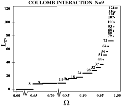
Figure 9: Ground-state angular momenta, $L_{\text{gs}}$, for $N=9$ bosons in a rapidly rotating trap [described by the LLL Hamiltonian in Eq. (3)], as a function of the rotational frequency $\Omega$ expressed in units of $\omega_{\bot}$. The bosons interact via a Coulombic repulsion and the many-body Hilbert space is restricted to the LLL. The angular momentum associated with the first bosonic Laughlin state occurs at $L=72$, i.e., at $N(N-1)$. The value of $c=0.2\hbar\omega_{\bot}\Lambda$ for this plot; the many-body wave functions do not depend on this choice. Unlike the case of a $\delta$-interaction (see Fig. 10), the values of the ground-state angular momenta do not terminate at $L=72$ (first Laughlin state), but they diverge as $\Omega/\omega_{\bot}\rightarrow 1$. Note the stepwise variation of the values of the ground-state angular momenta, indicating the presence of an intrinsic point-group symmetry associated with the polygonal-ring structure of RMBs (see text for details).

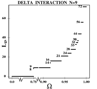
Figure 10: Ground-state angular momenta, $L_{\text{gs}}$, for $N=9$ bosons in a rapidly rotating trap [described by the LLL Hamiltonian in Eq. (3)], as a function of the rotational frequency $\Omega$ expressed in units of $\omega_{\bot}$. The bosons interact via a delta repulsion and the many-body Hilbert space is restricted to the LLL. The angular momentum associated with the first bosonic Laughlin state occurs at $L=72$, i.e., at $N(N-1)$. The value of $g=2\pi\hbar\omega_{\bot}\Lambda^{2}/N$ for this plot; the many-body wave functions do not depend on this choice. Unlike the case of a Coulomb interaction (see Fig. 9), the values of the ground-state angular momenta do terminate at $L=72$ (first Laughlin state) when $\Omega/\omega_{\bot}=1$. Note the stepwise variation of the values of the ground-state angular momenta, indicating the presence of an intrinsic point-group symmetry associated with the polygonal-ring structure of RMBs (see text for details).

Magic values dominate also the ground state angular momenta of neutral bosons (delta repulsion) in rotating traps, as shown for $N=6$ bosons in Fig. 2. Although the corresponding $\Omega$-ranges along the horizontal axis may be different compared to the Coulomb case, the appearance of only the two series $5k$ and $6k$ is remarkable – pointing to the formation of RBMs with similar $(1,5)$ and $(0,6)$ structures in the case of a delta interaction as well (see also Refs. mann ; barb ). An importance difference, however, is that for the delta interaction both series end at $\Omega/\omega_{\bot}=1$ with the value $L=N(N-1)=30$ (the bosonic Laughlin value at $\nu=1/2$), while for the Coulomb interaction this $L$ value is reached for $\Omega/\omega_{\bot}<1$ – allowing for an infinite set of magic angular momenta [larger than $N(N-1)$] to develop as $\Omega/\omega_{\bot}\rightarrow 1$. Later, we will return back to this important difference between long range and short range interactions.

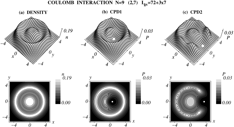
Figure 11: Single-particle density and CPDs for the ground state of $N=9$ bosons interacting via a Coulomb repulsion and having a total angular momentum of $L_{\text{gs}}=93$. The RBM crystalline structure corresponds to a $(2,7)$ polygonal-ring arrangement (which is the most stable classical equilibrium structure). Top row: contour plots. Bottom row: 3D plots. By column we describe the individual panels in both rows as follows: (a) Single-particle density. (b) CPD1 with reference point (indicated by a white dot) on the inner ring, revealing the localization of a second antipodal boson on the same inner ring. The outer ring exhibits a circular uniform symmetry that reflects the independent rotation of the two rings. (c) CPD2 with reference point on the outer ring revealing the localization of 6 bosons relative to the reference boson. We note that now the inner ring exhibits a uniform circular symmetry, reflecting again the independent rotation of the two rings. Lengths in units of $\Lambda$. The vertical scales are arbitrary, but the same in (b) and (c).

Beyond the analysis of the ground-state spectra as a function of $\Omega$, the intrinsic crystalline point-group structure can be revealed by an inspection of the CPDs [and to a much lesser extent by an inspection of single-particle densities]. Because the EXD many-body wave function is an eigenstate of the total angular momentum, the single-particle densities are circularly symmetric and can only reveal the presence of concentric rings through oscillations in the radial direction. The localization of bosons within the same ring can only be revealed via the azimuthal variations of the anisotropic CPD [Eq. (11)]. One of our findings is that for a given $N$ the crystalline features in the CPDs develop slowly as $L$ increases (or $\nu$ decreases).

For $\nu<1/2$, we find that the crystalline features are well developed for all sizes studied by us. In Fig. 3 and Fig. 4, we present some concrete examples of CPDs from EXD calculations associated with the ground-states of $N=6$ bosons in a rotating trap interacting via a repulsive Coulomb potential. In Fig. 3, we present the CPDs for $L_{\text{gs}}=30$ (bosonic Laughlin for $\nu=1/2$), 60, and 120; these angular momenta are associated with ground states at specific $\Omega$-ranges [see Fig. 1]. All three of these angular momenta are divisible by both 5 and 6. However, only the $L_{\text{gs}}=30$ CPD (Fig. 3 top row) has a structure that is intermediate between the $(1,5)$ and the $(0,6)$ polygonal-ring arrangements. The two other CPDs, associated with the higher $L_{\text{gs}}=60$ and $L_{\text{gs}}=120$ exhibit clearly only the $(1,5)$, illustrating our statement above that the quantum-mechanical CPDs conform to the structure of the most stable arrangement (i.e., the $(1,5)$ for $N=6$) of classical point-like charges as the fractional filling decreases. On the other hand, in Fig. 4, we plot the CPD for $L_{\text{gs}}=36$, which is divisible only by 6; we see that the corresponding single-particle density and CPD are associated with a $(0,6)$ polygonal-ring arrangement.

However, for $\nu>1/2$, the azimuthal variations may not be visible in the CPDs, in spite of the characteristic step-like ground-state spectra [see Fig. 1 for $N=6$ bosons and Fig. 9 for $N=9$ bosons]. This paradox is resolved when one considers higher-order correlations, and in particular $N$-point correlations [see Eq. (12)]. In Fig. 5 and Fig. 6, we plot the $N$-point correlation functions for $N=6$ bosons and $L_{\text{gs}}=12$ for both the Coulomb interaction and $\delta$-repulsion, respectively, and we compare them against the corresponding CPDs. The value of 12 is divisible by 6, and one expects this state to be associated with a $(0,6)$ molecular configuration. It is apparent that the CPDs fail to portray such sixfold azimuthal pattern. The $(0,6)$ pattern, however, is clear in the $N$-point correlations, where we fixed five points (white dots) at the positions ${\bf r}_{k}=r_{0}\exp(ik\pi/3)$, $k=1,2,...,5$ ($r_{0}$ being the radius of the maximum ring in the single-particle density) and we looked for the probability of finding the sixth boson at any other position ${\bf r}$. The figures show that the maximum probability happens for ${\bf r}_{6}=r_{0}\exp(2\pi i)$ (black dot) which completes the $(0,6)$ regular polygon.

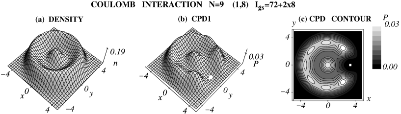
Figure 12: A ground state with a $(1,8)$ RBM arrangement for $N=9$ bosons interacting via a Coulomb repuslion and having angular momentum $L_{\text{gs}}=88$. In the classical calculation peeters_classical , this arrangement is isomeric to the most stable $(2,7)$ one exhibited by the CPDs in Fig. 11. The individual panels are as follows: (a) $3D$ plot of the single-particle density. (b) $3D$ plot of the CPD. (c) Contour plot of the CPD. In the CPD plots, the white dots indicate the reference point ${\bf r}_{0}$. Lengths in units of $\Lambda$. The vertical scales are arbitrary, but the same in (b) and (c).

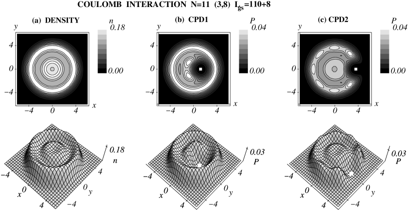
Figure 13: Single-particle density and CPDs for the ground state of $N=11$ bosons interacting via a Coulomb repulsion and having a total angular momentum of $L_{\text{gs}}=118$. The RBM crystalline structure corresponds to a $(3,8)$ polygonal-ring arrangement (which is the most stable classical equilibrium structure peeters_classical ). Top row: contour plots. Bottom row: 3D plots. By column we describe the individual panels in both rows as follows: (a) Single-particle density. (b) CPD with reference point (indicated by a white dot) on the inner ring, revealing the localization of two bosons on the same inner ring relative to the reference boson. The outer ring exhibits a circular uniform symmetry that reflects the independent rotation of the two rings. (c) CPD with reference point on the outer ring revealing the localization of 7 bosons relative to the reference boson. We note that now the inner ring exhibits a uniform circular symmetry, reflecting again the independent rotation of the two rings (see text for details). Lengths in units of $\Lambda$. The vertical scales are arbitrary, but the same in (b) and (c).

A second example is given in Fig. 7 and Fig. 8 for the case of $N=6$ bosons and $L_{\text{gs}}=15$,and for both the Coulomb interaction and the $\delta$-repulsion, respectively. In this second case, one expects a $(1,5)$ molecular pattern, which however is not visible in the CPDs. To reveal this $(1,5)$ pattern, one needs to plot the $N$-point correlations (middle and right panels). One now has two choices for choosing the positions of the first five particles (white dots), i.e., one choice places one white dot at the center and the other choice places all five white dots on the vertices of a regular pentagon. For both choices, as shown by the contour lines in the figures, the position of maximum probability for the sixth boson coincides with the point that completes the $(1,5)$ configuration [see the black dots at ${\bf r}_{6}=r_{0}\exp(2\pi i)$ in the middle panels and at the center in the right panels].

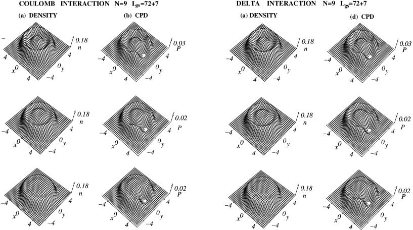
Figure 14: Comparison of single-particle densities and CPDs for three degenerate states (right half of figure) of $N=9$ bosons interacting via a repulsive $\delta$-interaction and having $L_{\text{gs}}=79$ against the lowest three (and non-degenerate) eigenstates (left half of figure) of the Coulomb repulsion for the same angular momentum. The numbers on the left hand side of the rows indicate the order of the eigenstates in the case of the Coulomb interaction, with 1 (top row) indicating the ground state, while 2 and 3 indicate excited (rovibrational yl7 ) states. The top-row plots reveal a $(2,7)$ crystalline $(2,7)$ structure for both types (long-range and short-range) interactions. Lengths in units of $\Lambda$. The vertical scales are arbitrary, but the same for the single-particle densities [(a) and (c)] and for the CPDs [(b) and (d)].

Note that for both cases, the differences in the CPDs and $N$-point correlation functions between the Coulomb and the $\delta$-repulsion are rather minimal. We will return to this result again in Section III.D.

III.2 The $N=9$ case with Coulomb repulsion

The results for $N=6$ bosons portray many of the important features for all the $N$’s that we have examined, keeping in mind that for $N=6$ the corresponding polygonal-ring structures involve only a single nontrivial ring, i.e., they are of the form $(1,5)$ or $(0,6)$. From the case of confined electrons yl4 ; yl5 , it is known that the first nontrivial two-ring structure appears for $N=9$. Our results presented here confirm that this is also the case for $N=9$ bosons.

In Fig. 9, we display the LLL ground-state angular momenta obtained from EXD calculations for $N=9$ bosons as a funtion of $\Omega/\omega_{0}$ and for the case of a Coulombic repulsion. The remarkable feature again is the variation of $L_{\text{gs}}$ in well defined steps, with the steps taking only three specific values 7, 8, and 9 (with the step value of 9 appearing only in two instances). The coresponding magic-angular-momenta values correspond to the series $L_{\text{gs}}=2k_{1}+7k_{2}$ (${\cal S}_{7}$), $L_{\text{gs}}=8k$ (${\cal S}_{8}$), and $L_{\text{gs}}=9k$ (${\cal S}_{9}$), associated with the polygonal-ring configurations $(2,7)$, $(1,8)$, and $(0,9)$, respectively. Note that, as $\Omega/\omega_{0}\rightarrow 1$, only the ${\cal S}_{7}$ series survives, a behavior that is again related to the fact that the $(2,7)$ structures is the most stable isomer according to classical elecrostatic calculations peeters_classical , with the $(1,8)$ structure being the lowest metastable isomer.

In Fig. 11, we present the single-particle density and CPD for $N=9$ bosons and $L_{\text{gs}}=93$ (with $k_{1}=1$ and $k_{2}=13$). Naturally, the single-particle density is circularly symmetric, but it clearly protrays two concentric rings along the radial direction. Furthermore, the$(2,7)$ intrinsic azimuthal crystalline pattern is revealed in the two displayed CPDs, one with the observation point being located on the inner ring (middle panels) and the other on the outer ring (right panels). It is remarkable that positioning the reference point ${\bf r}_{0}$ on one ring reveals only the intrinsic crystalline correlations of the same ring, while the other ring appears uniform, and vice versa. This behavior is similar to that of multi-ring rotating electron molecules yl4 ; yl5 , and it suggests that the rings of the RBMs rotate independently from each other. It naturally leads to a physical picture of the RBMs as highly nonrigid rotors in analogy with the analysis yl4 ; yl5 of the rotating electron molecules in high $B$ (see in particular sections V and VI in Ref. yl5 ).

We close this subsection by showing a case associated the second isomer. Fig. 12 displays the single-particle density and CPDs for $N=9$ bosons and $L_{\text{gs}}=88$ (belonging to the ${\cal S}_{8}$ series with $k=11$). Both of these quantities confirm that the ground state has a $(1,8)$ intrinsic crystalline pattern, in agreement with the analysis above regarding the ground-state angular-momentum spectrum in Fig. 9.

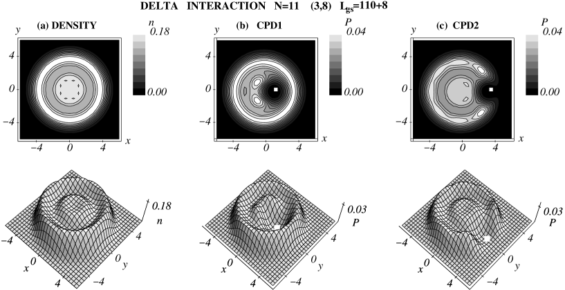
Figure 15: Single-particle density and CPDs for one of the degenerate ground state of $N=11$ bosons interacting via a delta repulsion and having a total angular momentum of $L_{\text{gs}}=118$. The RBM crystalline structure corresponds to a $(3,8)$ polygonal-ring arrangement (which is the most stable classical equilibrium structure peeters_classical ). Top row: contour plots. Bottom row: 3D plots. By column we describe the individual panels in both rows as follows: (a) Single-particle density. (b) CPD with reference point (indicated by a white dot) on the inner ring, revealing the localization of two bosons on the same inner ring relative to the reference boson. The outer ring exhibits a circular uniform symmetry that reflects the independent rotation of the two rings. (c) CPD with reference point on the outer ring revealing the localization of 7 bosons relative to the reference boson. We note that now the inner ring exhibits a uniform circular symmetry, reflecting again the independent rotation of the two rings (see text for details). Lengths in units of $\Lambda$. The vertical scales are arbitrary, but the same in (b) and (c).

III.3 The N=11 case with Coulomb repulsion

Figure 13 provides another example of the independent rotation of the rings that form the RBMs. In particular, Fig. 13 displays the single-particle density and the two CPDS (for the inner and outer ring) for $L_{\text{gs}}=118$ and $N=11$ bosons interacting via a Coulomb repulsive potential. The intrinsic crystalline structure has a $(3,8)$ pattern, in agreement with the decomposition of the total angular momentum as $118=3\times 2+8\times 14$ and the fact that the $(3,8)$ isomer is the most stable one according to classical electrostatic calculations peeters_classical .

III.4 Short-range vs. long-range interactions

In the present investigation, we also also studied the influence of the range of the interaction on the properties of the many-body wavefunctions associated with a finite number of rapidly rotating bosons. In particular, using both a Coulombic and a delta interaction, we have calculated and compared single-particle densities and CPDs for several sizes and fractional fillings $\nu$. Our result is that both types of interactions yield similar CPDs, i.e., that the degree of crystalline correlations does not depend strongly on the range of the interaction, as long as one refers to the same size $N$ and fractional filling $\nu$.

For example, the well developed crystallinity for $\nu<1/2$ familiar from the Coulombic case (see earlier sections) maintains also for the case of a $\delta$-interaction, as Fig. 14 ($N=9$) and Fig. 15 ($N=11$) illustrate. In particular, Fig. 14 compares for $N=9$ and $L=93$ the single-particle densities and CPDs associated with the three lowest states in the case of the Coulomb interaction (left half of the figure) against the corresponding quantities for three states out of the set of the now multiply degenerate vief ground states in the case of the $\delta$-interaction. Of course, this multiple degeneracy is unphysical, and in experimental applications one should use a short-range potential with a finite interaction length that is intermediate between the Coulomb and the $\delta$-potential, like the dipole-dipole interaction youl . For our purposes here, it is sufficient to view the $\delta$-interaction as a representative one of all short-range potentials, and thus to conclude that RBMs with similar patterns and properties do form, and that the degree of crystallinity is strengthened as $\nu$ decreases, for both long-range and short-range interactions. We stress that the similarities involve both the crystalline arrangements [i.e., the $(2,7)$ polygonal-ring pattern] and the property that the rings rotate independently of each other, as can be seen by a direct comparison of the left and right halves of Fig. 14. We note that certain similarities (regarding the formation of RBMs in the LLL) between the long-range (Coulomb) and short-range (Gaussian interaction) cases have also been reported mann most recently in the context of EXD/LLL studies of one-ring RBMs (with $N\leq 7$ and $\nu<1/2$). For similarities in the case $\nu\geq 1/2$, see Section III.A.

Finally Fig. 15 displays the CPD associated with one of the degenerate ground states for $L=118$ and $N=11$ bosons interacting via a $\delta$-potential. In keeping with our conclusions in the previous paragraph, we point out the clear formation of an RBM with a $(3,8)$ crystalline pattern; furthermore, this RBM also exhibits the property that the two rings rotate independently of each other.

IV Conclusions

We presented results for the exact diagonalization of a small number $N\leq 11$ of rapidly rotating bosons interacting via a repulsive $\delta$-function or Coulomb interaction. We focused on the weakly interacting limit where the assumption of confinement to the lowest Landau level is valid and studied in particular particle numbers which in the classical limit lead to polygonal crystalline configurations with at least two concentric polygonal rings. For all fractional fillings, we observed formation of rotating boson molecules, i.e., the appearance of crystalline correlations in close similarity to those found for confined two dimensional electron systems in high $B$ yl1 ; yl2 ; yl3 ; yl4 ; yl5 ; yl6 , as well as for trapped strongly repelling bosons in the context of a recently developed trial wave function yl11 ; yl13 .

Our main result is that for small filling fractions, i.e., $\nu<1/2$, the molecular character is well developed and explicit in the CPDs; for larger fractions $\nu\geq 1/2$, the molecular character is clearly revealed through inspection of higher-order correlation functions. The bosons organize into concentric polygonal rings which rotate independently of each other, as was earlier found yl4 ; yl5 for the case of rotating electron molecules in high $B$. The molecular structure is reflected in the ground-state spectra, i.e., as a function of the rotational frequency of the trap, the ground-state angular momenta vary in characteristic steps that coincide with the number of localized bosons on each polygonal ring note57 . Comparison of results for $\delta$-function and Coulomb interactions also indicates that the emergence of the RBM is more dependent on the fractional filling $\nu$ than on the range of the inter-particle interaction.

Appendix A Mathematical formalism and methods

A.1 formalism

Let

$$\Phi_{A}=\sqrt{\frac{n_{1}!n_{2}!\ldots n_{M}!}{N!}}\sum_{P}u_{P_{\alpha 1}}(1)u_{P_{\alpha 2}}(2)\ldots u_{P_{\alpha N}}(N),$$ (14)

represent one of the properly normalized permanents in Eq. (9) that form the basis of the many-body Hilbert space for the bosonic problem defined by the Hamiltonian in Eq. (3). Such a permanent is constructed with $M(\leq N)$ orthonormal single particle orbitals $u_{\alpha_{i}}(i)$ (LLL states in our case). The orbitals are indexed by a single integer $\alpha_{i}$ and $(i)$ stands for all coordinates of particle $i$. While $i=1,2,\ldots,N$, the indices $\alpha_{i}$ are not necessarily distinct. The summation $\sum_{P}$ runs over all distinct permutations of $N$ particles among the $M$ orbitals with occupations (multiplicities) $\{n_{1},n_{2},\ldots,n_{M}\}$.

It is straightforward to show that the permanent defined in Eq. (14) is normalized to unity. Indeed its norm is given by the following expression:

$$(\Phi_{A}^{*},\Phi_{A})=\int\prod_{i=1,N}d{\bf r}_{i}\frac{n_{1}!n_{2}!\ldots n_{M}!}{N!}$$

$$\times\sum_{P}\sum_{Q}u_{P_{\alpha_{1}}}^{*}(1)u_{Q_{\alpha_{1}}}(1)\dots u_{P_{\alpha_{N}}}^{*}(N)u_{Q_{\alpha_{N}}}(N),\qquad$$

(15)

which upon evaluating the integrals yields

$$(\Phi_{A}^{*},\Phi_{A}) = \frac{n_{1}!n_{2}!\ldots n_{M}!}{N!}\sum_{P}\sum_{Q}\delta_{{P_{\alpha_{1}}},{Q_{\alpha_{1}}}}\dots\delta_{P_{\alpha_{N}},Q_{\alpha_{N}}}$$

$$= \frac{n_{1}!n_{2}!\ldots n_{M}!}{N!}\sum_{P}(1)$$

$$= \frac{n_{1}!n_{2}!\ldots n_{M}!}{N!}\frac{N!}{n_{1}!n_{2}!\ldots n_{M}!}=1$$

where in the last line the summation equals the number of distinct ways of arranging $N$ particles among $M$ orbitals with the $j$th orbital having multiplicity $n_{j}$.

A.2 Interaction Matrix Elements

We make use of $\Phi_{A}$, i.e., Eq. (14) above, which represents a properly symmetrized and normalized wavefunction to calculate the matrix elements for the many-body interaction term which we denote here as

$$V_{\text{\text{I}}}=\sum_{i<j}v_{ij}.$$ (16)

At the outset we note that $v_{ij}=v({\bf r}_{i}-{\bf r}_{j})$ is symmetric with respect to the exchange of particles $i$ and $j$ and due to the symmetry of bosonic wavefunctions, this property is carried over to the expression:

$$(\Phi_{A}^{*}({\bf r}_{1},{\bf r}_{2},\ldots,{\bf r}_{N}),v_{ij}\Phi_{B}({\bf r}_{1},{\bf r}_{2},\ldots,{\bf r}_{N}))$$ (17)

In other words Eq. (17) doesn’t change value under exchange of all the coordinates of particles $i$ and $j$ with any other pair. So

$$\langle V_{\text{I}}\rangle_{AB}=\sum_{i<j}(\Phi_{A}^{*},v_{ij}\Phi_{B})=\frac{N(N-1)}{2}(\Phi_{A}^{*},v_{12}\Phi_{B})$$ (18)

and the matrix element for the many-body Hamiltonian due to the interaction is reduced to

$$\langle V_{\text{I}}\rangle_{AB}=\frac{N(N-1)}{2}(\Phi_{A}^{*},v_{12}\Phi_{B})$$ (19)

From our calculation of the norm in section A.1 above, it should be obvious that matrix element defined by Eq. (19) can be non-zero if $\Phi_{A}$ and $\Phi_{B}$ are the same or differ in the occupations of two orbitals from each one; the case when $\Phi_{A}$ and $\Phi_{B}$ differ in the occupations of one orbital from each permanent does not occur in the LLL. For all other cases the matrix elements in Eq. (19) are zero. Because of the normalization factors introduced by the occupation numbers $n_{j}$, the evaluation of Eq. (19) breaks down into five cases, one for the diagonal elements and four for the off-diagonal elements. We shall take them in turn.

A.3 Diagonal Elements

Substituting the expression for the normalized wavefunction Eq. (14) into (19) above, we obtain

$$\langle V_{\text{I}}\rangle_{AA} = \frac{N(N-1)}{2}\int\prod_{i=1,N}d{\bf r}_{i}\frac{n_{1}!\ldots n_{M}!}{N!}\sum_{P,Q}u_{P_{\alpha_{1}}}^{*}(1)u_{P_{\alpha_{2}}}^{*}(2)v_{12}u_{Q_{\alpha_{1}}}(1)u_{Q_{\alpha_{2}}}(2)\prod_{j=3,N}u_{P_{\alpha_{j}}}^{*}(j)u_{Q_{\alpha_{j}}}(j)\qquad$$ (20)

$$= \frac{N(N-1)}{2}\int d{\bf r}_{1}d{\bf r}_{2}\frac{n_{1}!n_{2}!\ldots n_{M}!}{N!}\sum_{P,Q}u_{P_{\alpha_{1}}}^{*}(1)u_{P_{\alpha_{2}}}^{*}(2)v_{12}u_{Q_{\alpha_{1}}}(1)u_{Q_{\alpha_{2}}}(2)\prod_{i=3,N}\delta_{P_{\alpha_{i}},Q_{\alpha_{i}}}$$

In Eq. (20) only two terms in the sum $\sum_{Q}$ can be nonzero, i.e., the terms satisfying the two conditions below

$$P_{\alpha_{1}}=Q_{\alpha_{1}}\;\text{and}\;P_{\alpha_{2}}=Q_{\alpha_{2}},\;\;\text{or}$$

$$P_{\alpha_{1}}=Q_{\alpha_{2}}\;\text{and}\;P_{\alpha_{2}}=Q_{\alpha_{1}};$$

and for both of the above cases

$$P_{\alpha_{j}}=Q_{\alpha_{j}},\;\;\;j=3,\ldots,N.$$ (21)

Thus Eq. (20) is rewritten as

$$\langle V_{\text{I}}\rangle_{AA}=\frac{n_{1}!\ldots n_{\alpha}!n_{\beta}!\ldots n_{M}!}{2(N-2)!}$$

$$\times\sum_{\alpha\beta}\biglb(\langle\alpha\beta|v_{12}|\alpha\beta\rangle+\langle\alpha\beta|v_{12}|\beta\alpha\rangle\bigrb)\sum_{P\{N-2\}}(1),$$

(22)

where we have simplified the notation of the indices, i.e., we set $P_{\alpha_{1}}=\alpha$ and $P_{\alpha_{2}}=\beta$, and we used the following shorthand definition for the matrix elements of the two-body interaction

$$\langle\alpha\beta|v_{12}|\gamma\Delta\rangle=\int d{\bf r}_{1}d{\bf r}_{2}u_{\alpha}^{*}(1)u_{\beta}^{*}(2)v_{12}u_{\gamma}(1)u_{\Delta}(2).$$ (23)

In Eq. (22), we have explicitly noted the fact that the sum $\sum_{P}$ refers now to $N-2$ particles. There are two case to be considered. When $\alpha=\beta$, one has

$$\sum_{P\{N-2\}}(1)=\frac{(N-2)!}{n_{1}!\ldots(n_{\alpha}-2)!n_{\beta}!\ldots n_{M}!}.$$ (24)

When $\alpha\neq\beta$, one has

$$\sum_{P\{N-2\}}(1)=\frac{(N-2)!}{n_{1}!\ldots(n_{\alpha}-1)!(n_{\beta}-1)!\ldots n_{M}!}.$$ (25)

With the above results, Eq. (22) finally yields for the diagonal elements of the interaction part of the Hamiltonian

$$\langle V_{\text{I}}\rangle_{AA} = \frac{n_{\alpha}(n_{\alpha}-1)}{2}\sum_{\alpha=1}^{M}\langle\alpha\alpha|v_{12}|\alpha\alpha\rangle$$

$$+ \frac{n_{\alpha}n_{\beta}}{2}\sum_{\alpha\neq\beta=1}^{M}\biglb(\langle\alpha\beta|v_{12}|\alpha\beta\rangle+\langle\alpha\beta|v_{12}|\beta\alpha\rangle\bigrb)$$

A.4 Off-Diagonal Elements

Here, we extend the formalism developed in the previous sections to be able to treat matrix elements between two different basis permanents. Let $\Phi_{\alpha\beta}^{\gamma\Delta}$ and $\Phi_{\alpha-1,\beta-1}^{\gamma+1,\Delta+1}$ denote permaments having the occupation numbers

$$\{n_{1},n_{2},\ldots,n_{\alpha},n_{\beta},n_{\gamma},n_{\Delta},\ldots,n_{M}\}$$ (27)

and

$$\{n_{1},n_{2},\ldots,n_{\alpha}-1,n_{\beta}-1,n_{\gamma}+1,n_{\Delta}+1,\ldots,n_{M}\},$$ (28)

respectively. Then we need to calculate the matrix element

$$(\Phi_{\alpha-1,\beta-1}^{\gamma+1,\Delta+1},V_{\text{I}}\Phi_{\alpha\beta}^{\gamma\Delta}).$$ (29)

$\Phi_{\alpha-1,\beta-1}^{\gamma+1,\Delta+1}$ can be interpreted as the permanent created from $\Phi_{\alpha\beta}^{\gamma\Delta}$ when two particles are taken from the single particle states labelled by $\alpha$ and $\beta$ and placed into the states $\gamma$ and $\Delta$. Four cases arise; they are

$$\gamma\;\neq\;\Delta;\;\;\alpha\;\neq\;\beta$$

$$\gamma\;\neq\;\Delta;\;\;\alpha\;=\;\beta$$

$$\gamma\;=\;\Delta;\;\;\alpha\;\neq\;\beta$$

$$\gamma\;=\;\Delta;\;\;\alpha\;=\;\beta$$ (30)

$\bullet$ Case I:  $\gamma\;\neq\;\Delta;\;\alpha\;\neq\;\beta$.
We begin from Eq. (19) and make adjustments for the difference in the occupation numbers to obtain:

$$(\Phi_{\alpha-1,\beta-1}^{*\gamma+1,\Delta+1},V_{\text{I}}\Phi_{\alpha\beta}^{\gamma\Delta})=$$

$$\frac{N(N-1)}{2}\sqrt{\frac{n_{1}!\ldots(n_{\alpha}-1)!(n_{\beta}-1)!(n_{\gamma}+1)!(n_{\Delta}+1)!\ldots n_{M}!}{N!}}\sqrt{\frac{n_{1}!\ldots n_{\alpha}!n_{\beta}!n_{\gamma}!n_{\Delta}!\ldots n_{M}!}{N!}}$$

$$\times\biglb(\langle\gamma\Delta|v_{12}|\alpha\beta\rangle+\langle\gamma\Delta|v_{12}|\beta\alpha\rangle+\langle\Delta\gamma|v_{12}|\alpha\beta\rangle+\langle\Delta\gamma|v_{12}|\beta\alpha\rangle\bigrb)\frac{(N-2)!}{n_{1}!\ldots(n_{\alpha}-1)!(n_{\beta}-1)!n_{\gamma}!n_{\Delta}!\ldots n_{M}!}$$

or finally

$$(\Phi_{\alpha-1,\beta-1}^{*\gamma+1,\Delta+1},V_{\text{I}}\Phi_{\alpha\beta}^{\gamma\Delta})=$$

$$\sqrt{n_{\alpha}n_{\beta}(n_{\gamma}+1)(n_{\Delta}+1)}\biglb(\langle\gamma\Delta|v_{12}|\alpha\beta\rangle+\langle\gamma\Delta|v_{12}|\beta\alpha\rangle\bigrb)$$ (32)

With similar considerations we obtain the results for the other cases.

$\bullet$ Case II: $\gamma\;\neq\;\Delta;\;\alpha\;=\;\beta$.

$$(\Phi_{\alpha-2}^{*\gamma+1,\Delta+1},V_{\text{I}}\Phi_{\alpha}^{\gamma\Delta})=$$

$$\frac{N(N-1)}{2}\sqrt{\frac{n_{1}!\ldots(n_{\alpha}-2)!(n_{\gamma}+1)!(n_{\Delta}+1)!\ldots n_{M}!}{N!}}\sqrt{\frac{n_{1}!\ldots n_{\alpha}!n_{\gamma}!n_{\Delta}!\ldots n_{M}!}{N!}}$$

$$\times\biglb(\langle\gamma\Delta|v_{12}|\alpha\alpha\rangle+\langle\Delta\gamma|v_{12}|\alpha\alpha\rangle\bigrb)\frac{(N-2)!}{n_{1}!\ldots(n_{\alpha}-2)!n_{\gamma}!n_{\Delta}!\ldots n_{M}!}$$

or finally

$$(\Phi_{\alpha-2}^{*\gamma+1,\Delta+1},V_{\text{I}}\Phi_{\alpha}^{\gamma\Delta})=$$

$$\sqrt{n_{\alpha}(n_{\alpha}-1)(n_{\gamma}+1)(n_{\Delta}+1)}\langle\gamma\Delta|v_{12}|\alpha\alpha\rangle$$

(34)

$\bullet$ Case III: $\gamma\;=\;\Delta;\;\alpha\;\neq\;\beta$.

$$(\Phi_{\alpha-1,\beta-1}^{*\gamma+2},V_{\text{I}}\Phi_{\alpha\beta}^{\gamma})=$$

$$\sqrt{n_{\alpha}n_{\beta}(n_{\gamma}+1)(n_{\gamma}+2)}\langle\gamma\gamma|v_{12}|\alpha\beta\rangle$$

(35)

$\bullet$ Case IV: $\gamma\;=\;\Delta;\;\alpha\;=\;\beta$.

$$(\Phi_{\alpha-2}^{*\gamma+2},V_{\text{I}}\Phi_{\alpha}^{\gamma})=$$

$$\frac{1}{2}\sqrt{n_{\alpha}(n_{\alpha}-1)(n_{\gamma}+1)(n_{\gamma}+2)}\langle\gamma\gamma|v_{12}|\alpha\alpha\rangle$$

(36)

A.5 Conditional probabilty distributions

If the many-body wave function is denoted as $\Psi({\bf r}_{1},{\bf r}_{2},\ldots,{\bf r}_{N})$, the conditional probability of finding a particle at position ${\bf r}$ given that there is another one at position ${\bf r}_{0}$ is given by

$$P({\bf r},{\bf r}_{0})=\frac{N(N-1)}{2}\int\prod_{i=3,N}d{\bf r}_{i}|\Psi({\bf r},{\bf r}_{0};{\bf r}_{3},\ldots,{\bf r}_{N})|^{2}.$$ (37)

We reduce the calculation of the conditional probability (within a proportionality constant) to evaluating the expectation value of the following two-body operator

$$T=\sum_{i\neq j}\delta({\bf r}-{\bf r}_{i})\delta({\bf r}_{0}-{\bf r}_{j}).$$ (38)

If ${\bf r}\neq{\bf r}_{0}$, the expression under the sum is not symmetric with respect to interchanging ${\bf r}_{i}$ and ${\bf r}_{j}$ [unlike the case of the two-body potential $v({\bf r}_{i}-{\bf r}_{j})$]. We rewrite $T$ as:

$$T = \sum_{i<j}\delta({\bf r}-{\bf r}_{i})\delta({\bf r}_{0}-{\bf r}_{j})+\sum_{j<i}\delta({\bf r}-{\bf r}_{i})\delta({\bf r}_{0}-{\bf r}_{j})$$

$$= \sum_{i<j}\biglb(\delta({\bf r}-{\bf r}_{i})\delta({\bf r}_{0}-{\bf r}_{j})+\delta({\bf r}-{\bf r}_{j})\delta({\bf r}_{0}-{\bf r}_{i})\bigrb).$$

which has a symmetric expression under the summation. Then the calculation of the CPD proceeds exactly as the calculation for the interaction part of the Hamiltonian.

References

- (1) F. Dalfovo, S. Giorgini, L.P. Pitaevskii, and S. Stringari, Rev. Mod. Phys. 71, 463 (1999).
- (2) A. J. Leggett, Rev. Mod. Phys. 73, 307 (2001).
- (3) T.L. Ho, Phys. Rev. Lett. 87, 060403 (2001).
- (4) A.L. Fetter, Phys. Rev. A 64, 063608 (2001).
- (5) C.J. Pethick and H. Smith, Bose-Einstein Condensation in Dilute Gases (Cambridge University Press, Cambridge, 2002).
- (6) L.P. Pitaevskii and S. Stringari, Bose-Einstein Condensation (Oxford University Press, Oxford, 2003).
- (7) L.O. Baksmaty, S.J. Woo, S. Choi, and N. P. Bigelow, Phys. Rev. Lett. 92, 160405 (2004).
- (8) S.J. Woo, L.O. Baksmaty, S. Choi, and N. P. Bigelow, Phys. Rev. Lett. 92, 170402 (2004).
- (9) G. Watanabe, G. Baym, and C.J. Pethick, Phys. Rev. Lett. 93, 190401 (2004).
- (10) G. Baym, J. Low Temp. Phys. 138, 601 (2005).
- (11) K.W. Madison, F. Chevy, W. Wohlleben, and J. Dalibard, Phys. Rev. Lett. 84, 806 (2000).
- (12) C. Raman, J.R. Abo-Shaeer, J.M. Vogels, K. Xu, and W. Ketterle, Phys. Rev. Lett. 87, 210402 (2001).
- (13) P. Engels, I. Coddington, P.C. Haljan, and E.A. Cornell, Phys. Rev. Lett. 89, 100403 (2002).
- (14) N.K. Wilkin and J.M.F. Gunn, Phys. Rev. Lett. 84, 6 (2000).
- (15) S. Viefers, T.H. Hansson, and S.M. Reimann, Phys. Rev. A 62, 053604 (2000).
- (16) N.R. Cooper, N.K. Wilkin, J.M.F. Gunn, Phys. Rev. Lett. 87, 120405 (2001).
- (17) N. Regnault and Th. Jolicoeur, Phys. Rev. Lett. 91, 030402 (2003).
- (18) C.C. Chang, N. Regnault, Th. Jolicoeur, and J.K. Jain, Phys. Rev. A 72, 013611 (2005).
- (19) C. Yannouleas and U. Landman, Phys. Rev. B 66, 115315 (2002).
- (20) C. Yannouleas and U. Landman, Phys. Rev. B 68, 035326 (2003).
- (21) C. Yannouleas and U. Landman, Phys. Rev. B 69, 113306 (2004).
- (22) C. Yannouleas and U. Landman, Phys. Rev. B 70, 235319 (2004).
- (23) Y.S. Li, C. Yannouleas, and U. Landman, Phys. Rev. B 73, 075301 (2006).
- (24) C. Yannouleas and U. Landman, phys. stat. sol. (a) 203, 1160 (2006).
- (25) W.Y. Ruan, Y.Y. Liu, C.G. Bao, and Z.Q. Zhang, Phys. Rev. B 51, 7942 (1995).
- (26) T. Seki, Y. Kuramoto, and T. Nishino, J. Phys. Soc. Jpn. 65, 3945 (1996).
- (27) P.A. Maksym, Phys. Rev. B 53, 10 871 (1996).
- (28) C. Yannouleas and U. Landman, Phys. Rev. Lett. 82, 5325 (1999).
- (29) R. Egger, W. Häusler, C.H. Mak, and H. Grabert, Phys. Rev. Lett. 82, 3320 (1999).
- (30) C. Yannouleas and U. Landman, Phys. Rev. Lett. 85, 1726 (2000).
- (31) S.A. Mikhailov, Phys. Rev. B 65, 115312 (2002).
- (32) C. Yannouleas and U. Landman, Phys. Rev. B 68, 035325 (2003).
- (33) C. Ellenberger, T. Ihn, C. Yannouleas, U. Landman, K. Ensslin, D. Driscoll, and A.C. Gossard, Phys. Rev. Lett. 96, 126806 (2006).
- (34) I. Romanovsky, C. Yannouleas and U. Landman, Phys. Rev. Lett. 93, 230405 (2004).
- (35) C. Yannouleas and U. Landman, Proc. Natl. Acad. Sci. (USA) 103, 10600 (2006).
- (36) I. Romanovsky, C. Yannouleas, L.O. Baksmaty, and U. Landman, Phys. Rev. Lett. 97, 090401 (2006).
- (37) S.M. Reimann, M. Koskinen, Y. Yu, and M. Manninen, New J. Phys. 8, 59 (2006).
- (38) N. Barberan, M. Lewenstein, K. Osterloh, and D. Dagnino, Phys. Rev. A 73, 063623 (2006).
- (39) The use of analytic variational (referred to also as trial) many-body wave functions restricted to the LLL has a long history starting with the Laughlin wave functions [see R.B. Laughlin, Phys. Rev. Lett. 50, 1395 (1983)]. For the derivation of analytic rotating-electron-molecule functions restricted to the LLL, see Ref. yl1 . For the generalization of the REM variational functions beyond the LLL, see Refs. yl3 ; yl5 .
- (40) For the definition of the fractional filling , we follow the fractional quantum Hall effect literature, see, e.g., S.M. Girvin and T. Sach, Phys. Rev. B 28, 4506 (1983).
- (41) M. Shellekens, R. Hoppeler, A. Perrin, J.V. Gomes, D. Boiron, A. Aspect, and C.I. Westbrook, Science 310, 648 (2005).
- (42) E. Altman, E. Demler, and M. D. Lukin, Phys. Rev. A 70, 013603 (2004).
- (43) S. Fölling, F. Gerber, A. Widera, O. Mandel, T. Gericke, and I. Bloch, Nature (London) 434, 481 (2005).
- (44) Ref. mann used a Gaussian-type two-body interaction in place of a contact potential.
- (45) EXD calculations for electrons in the LLL were also performed in M. Manninen, S. Viefers, M. Koskinen, and S.M. Reimann, Phys. Rev. B 64, 245322 (2001). These calculations were made in the same angular-momentum range () as the earlier Refs. seki ; maks . For extensive EXD calculations for electrons [covering the full range ], see Ref. yl2 ; such an extensive range is necessary for demonstrating the superiority of the REM interpretation for QDs under high compared to the composite-fermion and Jastrow-Laughlin “special-quantum-liquid” one (for the latter interpretation in the limited range , see J.K. Jain and T. Kawamura, Europhys. Lett. 29, 321 (1995), and also Refs. seki ; maks ).
- (46) Alex G. Morris and David L. Feder, e-print cond-mat/0602037.
- (47) V. Fock, Z. Phys. 47, 446 (1928).
- (48) C.G. Darwin, Proc. Cambridge Philos. Soc. 27, 86 (1930).
- (49) R. B. Lehoucq, D. C. Sorensen, and C. Yang, ARPACK Users’ Guide: Solution of Large-Scale Eigenvalue Problems with Implicitly Restarted Arnoldi Methods (SIAM, Philadelphia, 1998).
- (50) ARPACK was used in conjunction with PETSc (http://www.mcs.anl.gov/petsc) and SLEPc (http://www.grycap.upv.es/slepc).
- (51) For spin-polarized electrons in the LLL, the corresponding value is [see Refs. yl2 ; yl5 ].
- (52) M. Kong, B. Partoens, and F.M. Peeters, Phys. Rev. E 65, 046602 (2002).
- (53) A.H. MacDonald, S.R.E. Yang, and M.D. Johnson, Aust. J. Phys. 46, 345 (1993).
- (54) S. Yi and L. You, Phys. Rev. Lett. 92, 193201 (2004).
- (55) A single particle at the center does not count as an independent ring towards this rule.