Non-local effective medium of metamaterial

Abstract

In this paper, we investigate the effect of spatial dispersion on a double-lattice metamaterial which has both magnetic and electric response. A numerical scheme based on a dipolar model is developed to extract the non-local effective medium of the metamaterial. We found a structure-induced bianisotropy near the resonance gap even if the artificial particles are free from cross-coupling. A cross-coupled resonance also results from spatial dispersion and it can be understood using a Lorentz frequency dispersion model. The strength of the cross-coupled resonance depends on the microstructure and it is larger at a higher normalized frequency.

I Introduction

Metamaterials consisting arrays of artificial particles usually work in the frequency regime in which the free-space wavelength is larger than the inter-particle distance by a factor around 10. Their electromagnetic properties can therefore be understood by treating a metamaterial as a homogeneous medium. More often, a local effective medium of permittivity ($\epsilon_{eff}$) and permeability ($\mu_{eff}$) is assumed to be valid. There are several approaches in obtaining the local effective medium of a metamaterial. One approach is the S-parameter retrieval method. Smith:2005 It obtains the material parameters by comparing the transmission and the reflection coefficients of a slab of metamaterial and the corresponding homogeneous slab. Another approach relies on a homogenization theory which averages the microscopic field by line and area integrals. Pendry:1999 ; Smith:2006 ; Lerat:2006 Both approaches can cater for complex geometry and microstructure of the metamaterial and they work very well at frequencies far away from the resonance gap where spatial dispersion becomes important so that higher order eigenmodes (including the non-propagating ones) can be excited inside the metamaterial. Belov:2006 In this work, we will take another approach to deal with the spatial dispersion at a frequency near the resonance gap. Instead of picking or assuming a dominant eigenmode within the metamaterial, we will find the non-local effective medium directly for an arbitrary Bloch wave vector $\bf q$. For instance, the permittivity $\epsilon(\omega,{\bf q})$ now depends on both the angular frequency $\omega$ and the wave vector.

Apart from working near the resonance gap, some metamaterials like the wire medium , Belov:2003 ; Silveirinha:2006 the three-dimensional wire mesh Shapiro:2006 and the structured metal surface Garc:2005 also indicate that spatial dispersion (the non-local effective medium) can become important in order to have an accurate description of the metamaterial. In this paper, we will establish a numerical scheme in getting the non-local effective medium and some effects of spatial dispersion on metamaterial will be examined.

Section II outlines the numerical scheme in obtaining the non-local effective medium. We will employ a dipolar model for simplicity. It has the advantage that analytic formulas can be obtained in some cases. Moreover, all the material parameters, two tensors ($\mathord{\buildrel\lower 3.0pt\hbox{$\scriptscriptstyle\leftrightarrow$}\over{\epsilon}}$ and $\mathord{\buildrel\lower 3.0pt\hbox{$\scriptscriptstyle\leftrightarrow$}\over{\mu}}$) together with two pseudo tensors ($\mathord{\buildrel\lower 3.0pt\hbox{$\scriptscriptstyle\leftrightarrow$}\over{\xi}}$ and $\mathord{\buildrel\lower 3.0pt\hbox{$\scriptscriptstyle\leftrightarrow$}\over{\zeta}}$) can be obtained easily in the whole frequency regime. All the four constitutive tensors will be extracted as Ref. Marques:2002, and Xudong:2005, pointed out that a metamaterial should be described as a bianisotropic medium if the artificial atoms suffer from cross-coupling (electric field generates magnetic dipole and/or magnetic field generates electric dipole).

In Section III, the local effective medium of a double-lattice metamaterial will be first examined. One sublattice consists of electric artificial atoms and another sublattice consists of magnetic artificial atoms. The condition that the local effective medium becoming free of bianisotropy will be discussed.

In the last section, the non-local effective medium of the double-lattice metamaterial will be examined. The relationship between the non-local effective medium to the corresponding local one will be discussed. On the other hand, a Lorentz-type model is suggested for fitting the frequency dispersion of the non-local effective medium. Some effects of the spatial dispersion, including the structure-induced bianisotropy and the cross-coupled resonance, will also be discussed.

II Formulation

Here, we give an outline of the numerical scheme in obtaining the non-local effective medium using a dipolar model. The artificial particles ( split-rings, short wires, or electric atoms, Schurig:2006 etc.) are placed in an infinite lattice of lattice vectors ${\rm{\bf R}}$ in vacuum (of wavenumber $k_{0}$, wave speed $c_{0}$, and intrinsic impedance $\eta_{0})$. In each unit cell labeled by ${\rm{\bf R}}$, there are $n$ particles (indexed by $j=1,...,n)$ at positions ${\rm{\bf R}}+{\bf\tau}_{j}$. In the dipolar limit, each artificial particle has an electric dipole moment ${\rm{\bf p}}\left({{\rm{\bf R}}+{\rm{\bf\tau}}_{j}}\right)$ and a magnetic dipole moment ${\rm{\bf m}}\left({{\rm{\bf R}}+{\rm{\bf\tau}}_{j}}\right)$ and they are governed by the following equation (with time dependence factor $e^{-i\omega t}$ and S. I. units):

$$\left[{{\begin{array}[]{*{20}c}{c_{0}{\rm{\bf p}}\left({{\rm{\bf R}}+{\rm{\bf\tau}}_{j}}\right)\hfill}\\ {{\rm{\bf m}}\left({{\rm{\bf R}}+{\rm{\bf\tau}}_{j}}\right)\hfill}\\ \end{array}}}\right]={\alpha}_{j}\cdot\left[{{\begin{array}[]{*{20}c}{{\rm{\bf E}}_{\mbox{local}}\left({{\rm{\bf R}}+{\rm{\bf\tau}}_{j}}\right)/\eta_{0}\hfill}\\ {{\rm{\bf H}}_{\mbox{local}}\left({{\rm{\bf R}}+{\rm{\bf\tau}}_{j}}\right)\hfill}\\ \end{array}}}\right],$$ (1)

where ${{\rm{\bf E}}_{\mbox{local}}\left({{\rm{\bf R}}+{\rm{\bf\tau}}_{j}}\right)}$ and ${{\rm{\bf H}}_{\mbox{local}}\left({{\rm{\bf R}}+{\rm{\bf\tau}}_{j}}\right)}$ are the local electric and local magnetic fields at the center of the $j$-th particle. These local fields include the fields radiated by the external sources and the scattered fields from all the other particles. The 6-by-6 matrix ${\alpha}_{j}$ represents the polarizability of the $j$-th particle.

In this model, every artificial particle is replaced by an equivalent dipolar point particle. In order to extract the non-local effective medium of this crystal at an arbitrary wave vector ${\rm{\bf q}}$, we drive the crystal by the external fields in the form

$$\begin{split}{\rm{\bf E}}_{\mbox{ext}}\left({\rm{\bf r}}\right)&={\rm{\bf E}}_{\mbox{ext}}\exp\left({i{\rm{\bf q}}\cdot{\rm{\bf r}}}\right),\\ {\rm{\bf H}}_{\mbox{ext}}\left({\rm{\bf r}}\right)&={\rm{\bf H}}_{\mbox{ext}}\exp\left({i{\rm{\bf q}}\cdot{\rm{\bf r}}}\right).\\ \end{split}$$ (2)

These external fields are in fact generated by an electric and a magnetic polarization of the same spatial dependence. The crystal responds to it by generating dipole moments in the form

$$\left[{{\begin{array}[]{*{20}c}{c_{0}{\rm{\bf p}}\left({{\rm{\bf R}}+{\rm{\bf\tau}}_{j}}\right)\hfill}\\ {{\rm{\bf m}}\left({{\rm{\bf R}}+{\rm{\bf\tau}}_{j}}\right)\hfill}\\ \end{array}}}\right]=\left[{{\begin{array}[]{*{20}c}{c_{0}{\rm{\bf p}}_{j}\hfill}\\ {{\rm{\bf m}}_{j}\hfill}\\ \end{array}}}\right]e^{i{\rm{\bf q}}\cdot{\rm{\bf R}}},$$ (3)

which satisfies the multiple-scattering equation:

$$\sum\limits_{j^{\prime}=1}^{n}{\left({{T}^{-1}}\right)_{jj^{\prime}}\left({\rm{\bf q}}\right)}\cdot\frac{1}{V}\left[{{\begin{array}[]{*{20}c}{c_{0}{\rm{\bf p}}_{j^{\prime}}\hfill}\\ {{\rm{\bf m}}_{j^{\prime}}\hfill}\\ \end{array}}}\right]e^{-i{\rm{\bf q}}\cdot{\rm{\bf\tau}}_{j^{\prime}}}=\left[{{\begin{array}[]{*{20}c}{{\rm{\bf E}}_{\mbox{ext}}/\eta_{0}\hfill}\\ {{\rm{\bf H}}_{\mbox{ext}}\hfill}\\ \end{array}}}\right],$$ (4)

with $V$ being the volume of a single primitive unit cell. The $6n\times 6n$ transition matrix ${T}$ is given by its inverse:

$$\left({{T}^{-1}}\right)_{jj^{\prime}}\left({\rm{\bf q}}\right)=V{\alpha}_{j}^{-1}\delta_{jj^{\prime}}-{G}_{jj^{\prime}}\left({\rm{\bf q}}\right),$$ (5)

where the lattice Green’s function ${G}_{jj^{\prime}}$ is defined by

$${G}_{jj^{\prime}}\left({\rm{\bf q}}\right)=V\sum\limits_{{\rm{\bf r}}={\rm{\bf R}}+{\rm{\bf\tau}}_{j}-{\rm{\bf\tau}}_{j^{\prime}}\neq{\rm{\bf 0}}}{e^{-i{\rm{\bf q}}\cdot{\rm{\bf r}}}{G}_{0}\left({\rm{\bf r}}\right)}.$$ (6)

The 6-by-6 matrix ${G}_{0}\left({\rm{\bf r}}\right)$ which relates a dipole moment to its radiation field, together with its Fourier transform ${G}_{0}\left({\rm{\bf q}}\right)$ are given explicitly in Appendix A. The lattice Green’s function can be evaluated by the Ewald sum technique. For mathematical convenience, we also define

$${G}_{jj^{\prime}}\left({\rm{\bf q}}\right)+\frac{ik_{0}^{3}V}{6\pi}{I}\delta_{jj^{\prime}}={G}_{0}\left({\rm{\bf q}}\right)+\left[{{\begin{array}[]{*{20}c}{\mathord{\buildrel\lower 3.0pt\hbox{$\scriptscriptstyle\leftrightarrow$}\over{\beta}}_{jj^{\prime}}\left({\rm{\bf q}}\right)\hfill}&{\mathord{\buildrel\lower 3.0pt\hbox{$\scriptscriptstyle\leftrightarrow$}\over{\gamma}}_{jj^{\prime}}\left({\rm{\bf q}}\right)\hfill}\\ {-\mathord{\buildrel\lower 3.0pt\hbox{$\scriptscriptstyle\leftrightarrow$}\over{\gamma}}_{jj^{\prime}}\left({\rm{\bf q}}\right)\hfill}&{\mathord{\buildrel\lower 3.0pt\hbox{$\scriptscriptstyle\leftrightarrow$}\over{\beta}}_{jj^{\prime}}\left({\rm{\bf q}}\right)\hfill}\\ \end{array}}}\right],$$ (7)

where ${I}$ is the $6\times 6$ Identity Matrix. The tensors $\mathord{\buildrel\lower 3.0pt\hbox{$\scriptscriptstyle\leftrightarrow$}\over{\beta}}_{jj^{\prime}}\left({\rm{\bf q}}\right)$ and $\mathord{\buildrel\lower 3.0pt\hbox{$\scriptscriptstyle\leftrightarrow$}\over{\gamma}}_{jj^{\prime}}\left({\rm{\bf q}}\right)$ are periodic functions in the reciprocal space. They can be characterized according to the point group Dmitriev:2000 associated with the lattice structure at a particular wave vector ${\rm{\bf q}}$ together with the requirement that the matrix transpose (fixed $j$ and $j^{\prime}$) of $\mathord{\buildrel\lower 3.0pt\hbox{$\scriptscriptstyle\leftrightarrow$}\over{\gamma}}_{jj^{\prime}}\left({\rm{\bf q}}\right)$ satisfies

$$\mathord{\buildrel\lower 3.0pt\hbox{$\scriptscriptstyle\leftrightarrow$}\over{\gamma}}_{jj^{\prime}}\left({\rm{\bf q}}\right)^{T}=-\mathord{\buildrel\lower 3.0pt\hbox{$\scriptscriptstyle\leftrightarrow$}\over{\gamma}}_{jj^{\prime}}\left({\rm{\bf q}}\right),$$ (8)

which is already implied from Eq. (6) with Eq. (42) . Table 1 lists the forms of the tensors $\mathord{\buildrel\lower 3.0pt\hbox{$\scriptscriptstyle\leftrightarrow$}\over{\beta}}_{jj^{\prime}}\left({\rm{\bf q}}\right)$ and $\mathord{\buildrel\lower 3.0pt\hbox{$\scriptscriptstyle\leftrightarrow$}\over{\gamma}}_{jj^{\prime}}\left({\rm{\bf q}}\right)$ for some common single lattices and double lattices. The matrices are listed with respect to the Cartesian basis vectors $\left\{{\hat{x},\hat{y},\hat{z}}\right\}$ where $\hat{z}$ is defined to be the direction along ${\rm{\bf q}}$ in our convention.

	${\rm{\bf q}}$	$\mathord{\buildrel\lower 3.0pt\hbox{$\scriptscriptstyle\leftrightarrow$}\over{\beta}}_{jj^{\prime}}\left({\rm{\bf q}}\right)$	$\mathord{\buildrel\lower 3.0pt\hbox{$\scriptscriptstyle\leftrightarrow$}\over{\gamma}}_{jj^{\prime}}\left({\rm{\bf q}}\right)$
SC/ FCC/ BCC single lattice structure	At $\Gamma$	$\beta$	0
	Along [111]/[001]	$\left[{{\begin{array}[]{ccc}{\beta_{T}\hfill}&0\hfill&0\hfill\\ 0\hfill&{\beta_{T}\hfill}&0\hfill\\ 0\hfill&0\hfill&{\beta_{L}\hfill}\\ \end{array}}}\right]$	$\left[{{\begin{array}[]{*{20}c}0\hfill&{-\gamma\hfill}&0\hfill\\ \gamma\hfill&0\hfill&0\hfill\\ 0\hfill&0\hfill&0\hfill\\ \end{array}}}\right]$
NaCl/ CsCl	At $\Gamma$	$\beta$	0
	Along [111]/[001]	$\left[{{\begin{array}[]{*{20}c}{\beta_{T}\hfill}&0\hfill&0\hfill\\ 0\hfill&{\beta_{T}\hfill}&0\hfill\\ 0\hfill&0\hfill&{\beta_{L}\hfill}\\ \end{array}}}\right]$	$\left[{{\begin{array}[]{*{20}c}0\hfill&{-\gamma\hfill}&0\hfill\\ \gamma\hfill&0\hfill&0\hfill\\ 0\hfill&0\hfill&0\hfill\\ \end{array}}}\right]$
Zn Blende	At $\Gamma$	$\beta$	0
	Along [111]	$\left[{{\begin{array}[]{*{20}c}{\beta_{T}\hfill}&0\hfill&0\hfill\\ 0\hfill&{\beta_{T}\hfill}&0\hfill\\ 0\hfill&0\hfill&{\beta_{L}\hfill}\\ \end{array}}}\right]$	$\left[{{\begin{array}[]{*{20}c}0\hfill&{-\gamma\hfill}&0\hfill\\ \gamma\hfill&0\hfill&0\hfill\\ 0\hfill&0\hfill&0\hfill\\ \end{array}}}\right]$
	Along [001]: $\hat{x}\parallel\left[{110}\right]$, $\hat{y}\parallel\left[{-110}\right]$	$\left[{{\begin{array}[]{*{20}c}{\beta_{xx}\hfill}&0\hfill&0\hfill\\ 0\hfill&{\beta_{yy}\hfill}&0\hfill\\ 0\hfill&0\hfill&{\beta_{L}\hfill}\\ \end{array}}}\right]$	$\left[{{\begin{array}[]{*{20}c}0\hfill&{-\gamma\hfill}&0\hfill\\ \gamma\hfill&0\hfill&0\hfill\\ 0\hfill&0\hfill&0\hfill\\ \end{array}}}\right]$

Table 1: The tensor forms of the lattice Green’s function for different single and double lattice structures along different directions of the wave vector.

In the next step, the dipole moment distributions numerically solved from Eq. (4) are then macroscopically averaged. The procedure we choose here is to apply a low pass filter such that all the Fourier components outside the first Brillouin zone are eliminated. In essence, it means that all the microscopic fields are ensemble averaged by translating the whole crystal with an arbitrary distance while the external fields remain unchanged. Thus, the macroscopic polarizations are written as

$$\begin{split}c_{0}\left\langle{\rm{\bf P}}\right\rangle\left({\rm{\bf r}}\right)&=c_{0}\left\langle{\rm{\bf P}}\right\rangle e^{i{\rm{\bf q}}\cdot{\rm{\bf r}}}=\frac{1}{V}\sum\limits_{j=1}^{n}{c_{0}{\rm{\bf p}}_{j}e^{-i{\rm{\bf q}}\cdot{\rm{\bf\tau}}_{j}}}e^{i{\rm{\bf q}}\cdot{\rm{\bf r}}},\\ \left\langle{\rm{\bf M}}\right\rangle\left({\rm{\bf r}}\right)&=\left\langle{\rm{\bf M}}\right\rangle e^{i{\rm{\bf q}}\cdot{\rm{\bf r}}}=\frac{1}{V}\sum\limits_{j=1}^{n}{{\rm{\bf m}}_{j}e^{-i{\rm{\bf q}}\cdot{\rm{\bf\tau}}_{j}}}e^{i{\rm{\bf q}}\cdot{\rm{\bf r}}}.\\ \end{split}$$ (9)

The macroscopic polarizations can now be formally written as

$$\left[{{\begin{array}[]{*{20}c}{c_{0}\left\langle{\rm{\bf P}}\right\rangle\hfill}\\ {\left\langle{\rm{\bf M}}\right\rangle\hfill}\\ \end{array}}}\right]=\left\langle{T}\right\rangle\left({\rm{\bf q}}\right)\left[{{\begin{array}[]{*{20}c}{{\rm{\bf E}}_{\mbox{ext}}/\eta_{0}\hfill}\\ {{\rm{\bf H}}_{\mbox{ext}}\hfill}\\ \end{array}}}\right],$$ (10)

where the averaged transition matrix is given by

$$\left\langle{T}\right\rangle\left({\rm{\bf q}}\right)=\sum\limits_{j,{j^{\prime}}=1}^{n}{{T}_{jj^{\prime}}\left({\rm{\bf q}}\right)}.$$ (11)

Eq. (10) summarizes the response of the crystal to the external fields. Then, the macroscopic fields are constructed from the sum of the external fields and the secondary radiation by

$$\left[{{\begin{array}[]{*{20}c}{\left\langle{\rm{\bf E}}\right\rangle/\eta_{0}\hfill}\\ {\left\langle{\rm{\bf H}}\right\rangle\hfill}\\ \end{array}}}\right]={G}_{0}\left({\rm{\bf q}}\right)\cdot\left[{{\begin{array}[]{*{20}c}{c_{0}\left\langle{\rm{\bf P}}\right\rangle\hfill}\\ {\left\langle{\rm{\bf M}}\right\rangle\hfill}\\ \end{array}}}\right]+\left[{{\begin{array}[]{*{20}c}{{\rm{\bf E}}_{\mbox{ext}}/\eta_{0}\hfill}\\ {{\rm{\bf H}}_{\mbox{ext}}\hfill}\\ \end{array}}}\right].$$ (12)

Finally, by combining Eq. (10) and Eq. (12), we obtain the constitutive relationship

$$\left[{{\begin{array}[]{*{20}c}{c_{0}\left\langle{\rm{\bf P}}\right\rangle\hfill}\\ {\left\langle{\rm{\bf M}}\right\rangle\hfill}\\ \end{array}}}\right]={\left[{{\begin{array}[]{*{20}c}{\mathord{\buildrel\lower 3.0pt\hbox{$\scriptscriptstyle\leftrightarrow$}\over{\epsilon}}\left({\rm{\bf q}}\right)-\mathord{\buildrel\lower 3.0pt\hbox{$\scriptscriptstyle\leftrightarrow$}\over{I}}\hfill}&{\mathord{\buildrel\lower 3.0pt\hbox{$\scriptscriptstyle\leftrightarrow$}\over{\xi}}\left({\rm{\bf q}}\right)\hfill}\\ {\mathord{\buildrel\lower 3.0pt\hbox{$\scriptscriptstyle\leftrightarrow$}\over{\zeta}}\left({\rm{\bf q}}\right)\hfill}&{\mathord{\buildrel\lower 3.0pt\hbox{$\scriptscriptstyle\leftrightarrow$}\over{\mu}}\left({\rm{\bf q}}\right)-\mathord{\buildrel\lower 3.0pt\hbox{$\scriptscriptstyle\leftrightarrow$}\over{I}}\hfill}\\ \end{array}}}\right]}\cdot\left[{{\begin{array}[]{*{20}c}{\left\langle{\rm{\bf E}}\right\rangle/\eta_{0}\hfill}\\ {\left\langle{\rm{\bf H}}\right\rangle\hfill}\\ \end{array}}}\right],$$ (13)

where the four constitutive tensors are given by

$$\left[{{\begin{array}[]{*{20}c}{\mathord{\buildrel\lower 3.0pt\hbox{$\scriptscriptstyle\leftrightarrow$}\over{\epsilon}}\left({\rm{\bf q}}\right)-\mathord{\buildrel\lower 3.0pt\hbox{$\scriptscriptstyle\leftrightarrow$}\over{I}}\hfill}&{\mathord{\buildrel\lower 3.0pt\hbox{$\scriptscriptstyle\leftrightarrow$}\over{\xi}}\left({\rm{\bf q}}\right)\hfill}\\ {\mathord{\buildrel\lower 3.0pt\hbox{$\scriptscriptstyle\leftrightarrow$}\over{\zeta}}\left({\rm{\bf q}}\right)\hfill}&{\mathord{\buildrel\lower 3.0pt\hbox{$\scriptscriptstyle\leftrightarrow$}\over{\mu}}\left({\rm{\bf q}}\right)-\mathord{\buildrel\lower 3.0pt\hbox{$\scriptscriptstyle\leftrightarrow$}\over{I}}\hfill}\\ \end{array}}}\right]^{-1}=\left\langle{T}\right\rangle^{-1}\left({\rm{\bf q}}\right)+{G}_{0}\left({\rm{\bf q}}\right).$$ (14)

In general, apart from the permittivity tensor $\mathord{\buildrel\lower 3.0pt\hbox{$\scriptscriptstyle\leftrightarrow$}\over{\epsilon}}\left({\rm{\bf q}}\right)$ and the permeability tensor $\mathord{\buildrel\lower 3.0pt\hbox{$\scriptscriptstyle\leftrightarrow$}\over{\mu}}\left({\rm{\bf q}}\right)$, we also obtain the off-diagonal tensors $\mathord{\buildrel\lower 3.0pt\hbox{$\scriptscriptstyle\leftrightarrow$}\over{\xi}}\left({\rm{\bf q}}\right)$ and $\mathord{\buildrel\lower 3.0pt\hbox{$\scriptscriptstyle\leftrightarrow$}\over{\zeta}}\left({\rm{\bf q}}\right)$ which represent the bianisotropy of the metamaterial. We will see in the next section that the bianisotopy should not be neglected in considering the non-local effective medium. All the four tensors are functions of the frequency $\omega$ and the wave vector ${\rm{\bf q}}$. For convenience, we will omit writing $\omega$ inside the parenthesis for the constitutive tensors. Moreover, we will further omit the dependence of ${\rm{\bf q}}$ if the local limit ${\rm{\bf q}}={\rm{\bf 0}}$ is taken, i.e. $\mathord{\buildrel\lower 3.0pt\hbox{$\scriptscriptstyle\leftrightarrow$}\over{\epsilon}}\left({{\rm{\bf q}}={\rm{\bf 0}}}\right)$ is abbreviated as $\mathord{\buildrel\lower 3.0pt\hbox{$\scriptscriptstyle\leftrightarrow$}\over{\epsilon}}$.

We note that in our scheme of defining the non-local effective medium at a particular ${\rm{\bf q}}$, a fixed form of external fields (Eq. (2)) is used. There are alternative methods which directly deal with the macroscopic fields without considering the external fields. Ponti:2001 ; Ponti:2002

III The local effective medium - double lattice

In this work, we will concentrate on the double lattice structure which is a common type of microstructures for metamaterials in obtaining a negative refractive index. The double lattice consists of two types of artificial particles. One type of the particles (labeled by $j=1)$ has a resonating electric response (e.g. a short wire) and another (labeled by $j=2)$ has a resonating magnetic response (e.g. a split-ring). In particular, we would like to study the importance of the electro-magnetic coupling between the electric and the magnetic particles when we have a crystal structure having both electric and magnetic response. It is a general feature of metamaterials.

First, we would like to restrict our discussion to the class of metamaterials whose local effective medium is free from bianisotropy. It can be achieved through a careful design of the artificial particles such that the particles are free from cross-coupling. Juan:2004 ; Schurig:2006 Moreover, the lattice structure has to be carefully chosen as well. In fact, all the double lattice structures listed in Table 1 have vanishing $\mathord{\buildrel\lower 3.0pt\hbox{$\scriptscriptstyle\leftrightarrow$}\over{\gamma}}_{jj^{\prime}}$ at ${\rm{\bf q}}={\rm{\bf 0}}$. From Eq. (5), Eq. (11) and Eq. (14), it means that

$$\mathord{\buildrel\lower 3.0pt\hbox{$\scriptscriptstyle\leftrightarrow$}\over{\xi}}\left({{\rm{\bf q}}={\rm{\bf 0}}}\right)=\mathord{\buildrel\lower 3.0pt\hbox{$\scriptscriptstyle\leftrightarrow$}\over{\zeta}}\left({{\rm{\bf q}}={\rm{\bf 0}}}\right)=0.$$ (15)

For simplicity, we further assume that the electric particle can only be electrically polarized along the x-direction with polarizability $\alpha_{e}$ ($c_{0}p_{1x}=\alpha_{e}E_{local,x}(\bf{\tau}_{1})/\eta_{0}$), the magnetic particle can only be magnetically polarized along the y-direction with polarizability $\alpha_{m}$ ($m_{2y}=\alpha_{m}H_{local,y}(\bf{\tau}_{2})$) and all the polarizabilities along the other directions are assumed to be negligible. In this case, the relevant basis vectors can be reduced to $\left\{{c_{0}p_{1x},m_{2y}}\right\}$ in Eq. (4). Eq. (10) in the local limit can then be written as

$$\left\langle{T}\right\rangle^{-1}\left({{\rm{\bf q}}={\rm{\bf 0}}}\right)\left[{{\begin{array}[]{*{20}c}{c_{0}\left\langle{P_{x}}\right\rangle\hfill}\\ {\left\langle{M_{y}}\right\rangle\hfill}\\ \end{array}}}\right]=\left[{{\begin{array}[]{*{20}c}{E_{\mbox{ext,x}}/\eta_{0}\hfill}\\ {H_{\mbox{ext,y}}\hfill}\\ \end{array}}}\right],$$ (16)

where

$$\begin{array}[]{l}\left\langle{T}\right\rangle^{-1}\left({{\rm{\bf q}}={\rm{\bf 0}}}\right)+{G}_{0}\left({{\rm{\bf q}}={\rm{\bf 0}}}\right)=\\ \left[{{\begin{array}[]{*{20}c}{V\alpha_{e}^{-1}+\frac{ik_{0}^{3}V}{6\pi}-\beta_{T}\hfill}&0\hfill\\ 0\hfill&{V\alpha_{m}^{-1}+\frac{ik_{0}^{3}V}{6\pi}-\beta_{T}\hfill}\\ \end{array}}}\right],\end{array}$$ (17)

is now written in the $\left\{{c_{0}\left\langle{P_{x}}\right\rangle,\left\langle{M_{y}}\right\rangle}\right\}$ basis. The macroscopic electric polarization $\left\langle{\rm{\bf P}}\right\rangle$ is only contributed from the first particle while the macroscopic magnetic polarization $\left\langle{\rm{\bf M}}\right\rangle$ is only contributed from the second particle. Therefore, the local effective medium is governed by

$$\begin{split}\frac{1}{\epsilon_{T}-1}+\beta_{T}&=V\alpha_{e}^{-1}+ik_{0}^{3}V/\left({6\pi}\right),\\ \frac{1}{\mu_{T}-1}+\beta_{T}&=V\alpha_{m}^{-1}+ik_{0}^{3}V/\left({6\pi}\right).\\ \end{split}$$ (18)

Because of the carefully chosen microstructure, the local effective medium has exactly the same form to a single lattice of one type of particles. Belov:2005 This is the ideal case that the electric and the magnetic particles cannot “see” each other. Here, $\beta_{T}$ is the local limit (${\bf q}={\bf 0}$) of $\beta_{T}\left({\rm{\bf q}}\right)$ defined in Eq. (7). It is a function of the normalized frequency $\omega a/\left({2\pi c_{0}}\right)$ for the lattice structure and it can be well approximated by a polynomial at small frequencies. Table 2 gives the polynomial expansion of $\beta_{T}$ for various lattice structures. Note that for cubic lattices, $\beta_{T}\to 1/3$ at the long wavelength limit so that Eq. (18) returns to the Clausius-Mossotti equation. Tretyakov:2003 ; Mahan:2006

	$\beta_{T}$
SC	$1/3-5.97\Omega^{2}+11.8\Omega^{4}$
FCC	$1/3-2.40\Omega^{2}+1.72\Omega^{4}$
BCC	$1/3-3.82\Omega^{2}+4.38\Omega^{4}$

Table 2: Polynomial expansion of $\beta_{T}$ for different single lattices. The normalized frequency is $\Omega=\omega a/\left({2\pi c_{0}}\right)$ and $a$ is the lattice constant.

One popular form of the frequency dispersions of the local effective medium is given by

$$\begin{split}\epsilon_{T}=1-\frac{A\omega_{e}^{2}}{\omega^{2}-\omega_{e}^{2}+i\omega\Gamma_{e}},\\ \mu_{T}=1-\frac{B\omega^{2}}{\omega^{2}-\omega_{m}^{2}+i\omega\Gamma_{m}}.\\ \end{split}$$ (19)

Here, Eq. (19) is still called the Lorentz-model dispersion although the resonance term in permeability is modified so that these frequency dispersion forms give us the correct low frequency behavior (including the frequency regime near resonance) when there are only one electric resonance and one magnetic resonance. Boardman:2006 One point to note here is that for a passive particle, we have to satisfy $Im\left({1/\alpha_{e}}\right)\leq-k_{0}^{3}/\left({6\pi}\right)$ for the electric polarizability and also a similar inequality for the magnetic polarizability. Tretyakov_book:2003 It guarantees a positive imaginary part for both the local permittivity and the local permeability according to Eq. (18), i.e. $\Gamma_{e}$ or $\Gamma_{m}$ should be zero for a lossless medium or positive for a lossy medium under the dipolar model.

In the following, we would like to specify the local effective medium {$\epsilon_{T}$, $\mu_{T}$} directly instead of specifying the polarizabilities {$\alpha_{e}$, $\alpha_{m}$}. As an example, we consider the case that $\omega_{e}/\left({2\pi}\right)=8GHz$, $A=0.89$, $\omega_{m}/\left({2\pi}\right)=8.5GHz$, $B=0.128$ and $\Gamma_{e}=\Gamma_{m}=0$. The underlying microstructure is assumed to be a CsCl structure of lattice constant $a=5mm$. The polarizabilities can be found by Eq. (18) whenever a microscopic description is necessary. Fig. 1(a) and (b) show the local effective permittivity and the local permeability. Fig. 1(c) shows the crystal being viewed from the direction [001] or [010]. The uniaxial electric particle (green color) can be polarized along the [100] direction and the uniaxial magnetic particle can be polarized along the [010] direction. We will start from this configuration in the next section when we consider the non-local effective medium.

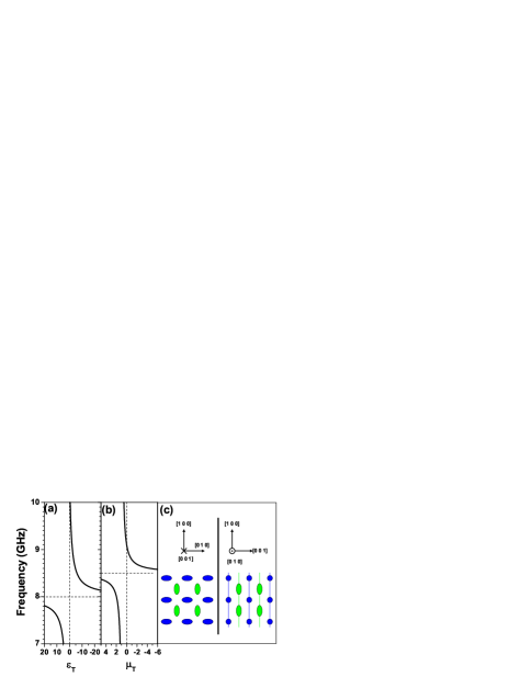
Figure 1: (Color online)A double-lattice configuration specified by Eq. (19) with $\omega_{e}/\left({2\pi}\right)=8GHz$, $A=0.89$, $\omega_{m}/\left({2\pi}\right)=8.5GHz$, $B=0.128$, $\Gamma_{e}=\Gamma_{m}=0$ and lattice constant a= 5 mm. (a) local permittivity; (b) local permeability; (c) The underlying CsCl structure viewed along the [001] and the [010] direction. The uniaxial electric particle (green color) can be polarized along the [100] direction. The uniaxial magnetic particle (blue color) can be polarized along the [010] direction.

It is more convenient to specify the metamaterial by its local effective medium directly. However, a note has to be taken for the freedom of the parameters in the frequency dispersion. In particular, for a non-absorptive particle, the polarizability can be written in terms of the dipolar scattering phase shift $\delta_{1}^{\left(\sigma\right)}$ (a real number) by

$$\frac{ik_{0}^{3}\alpha_{\sigma}}{3\pi}=\exp\left({2i\delta_{1}^{\left(\sigma\right)}}\right)-1,$$ (20)

where $\sigma=e,m$ for “e” wave scattering (non-zero local electric field with vanishing local magnetic field at the particle) or “m” wave scattering (non-zero local magnetic field with vanishing local electric field at the particle). Due to the finite volume of one single unit cell, the phase shift $\delta_{1}^{\left(\sigma\right)}$ cannot vary arbitrarily against frequency. Suppose a sphere of radius $r_{s}$ can completely enclose one artificial electric particle, the restriction on $\delta_{1}^{\left(e\right)}$ can be written in terms of the time-averaged total energy $\mathscr{E}$ within the enclosing sphere (for a quasi-monochromatic electromagnetic field) as:

$$\begin{split}\omega^{3}\mathscr{E}\propto&\omega\frac{d\delta_{1}^{\left(e\right)}}{d\omega}-\frac{1}{2\theta^{3}}(1+2\theta^{2}-2\theta^{4}-\cos 2\left({\theta+\delta_{1}^{\left(e\right)}}\right)\\ &-2\theta\sin 2\left({\theta+\delta_{1}^{\left(e\right)}}\right))\geq 0,\end{split}$$ (21)

where $\theta=\omega r_{s}/c_{0}$. See Appendix B for the derivation. This inequality must be satisfied. Otherwise, we can extract energy from the artificial particle without first pumping energy to it.

Figure 2: The time-averaged total electromagnetic energy within a sphere of (a)$r_{s}=1.4mm$ and (b) $r_{s}=2.0mm$ enclosing the electric particle for “e” wave scattering.

For our example, the polarizabilities are obtained through Eq. (18) and the time-averaged total energy for “e” wave scattering (in an arbitrary unit) is obtained from Eq. (20) and Eq. (21). Fig. 2 shows the results for two different cases. The solid line shows the case with $r_{s}=2mm$. The total energy within the sphere is positive in the whole frequency regime. The dashed line shows the case with a smaller radius $r_{s}=1.4mm$. In this case, the energy becomes negative which is not valid. Therefore, in order to design our metamaterial, the electric artificial particle must have a certain minimum size. On the other hand, if we already know the size of the electric artificial particle, it imposes a maximum on the electric resonance strength $A$ (in Eq. (19)) that the metamaterial can have.

IV The non-local effective medium – double lattice

In this section, we investigate how the effective medium changes when the wave vector is deviated from the Brillouin zone center. In fact, the tensor $\mathord{\buildrel\lower 3.0pt\hbox{$\scriptscriptstyle\leftrightarrow$}\over{\gamma}}_{12}\left({\rm{\bf q}}\right)$ does not vanish in general. For the double lattice we considered in the last section with ${\rm{\bf q}}$ along direction [111] or [100]/[010]/[001], Eq. (10) can still be written in the form of Eq. (16) where

$$\begin{array}[]{l}\left({\left\langle{T}\right\rangle^{-1}+{G}_{0}}\right)\left({\rm{\bf q}}\right)=\\ \left[{{\begin{array}[]{*{20}c}{V\alpha_{e}^{-1}+\frac{ik_{0}^{3}V}{6\pi}-\beta_{T}\left({\omega,{\rm{\bf q}}}\right)\hfill}&{\gamma_{12}\left({\omega,{\rm{\bf q}}}\right)\hfill}\\ {\gamma_{12}^{\ast}\left({\omega,{\rm{\bf q}}}\right)\hfill}&{V\alpha_{m}^{-1}+\frac{ik_{0}^{3}V}{6\pi}-\beta_{T}\left({\omega,{\rm{\bf q}}}\right)\hfill}\\ \end{array}}}\right].\end{array}$$ (22)

This 2-by-2 matrix is in the $\left\{{c_{0}\left\langle{P_{x}}\right\rangle,\left\langle{M_{y}}\right\rangle}\right\}$ basis with $\hat{z}$ being the direction along ${\rm{\bf q}}$, $\hat{x}$ being the direction the uniaxial electric particle can be polarized and $\hat{y}$ being the direction the uniaxial magnetic particle can be polarized. Therefore, by comparing to Eq. (17), the non-local effective medium can be written with respect to the local effective medium by

$$\begin{split}&\left[{{\begin{array}[]{*{20}c}{\epsilon_{T}\left({\rm{\bf q}}\right)-1\hfill}&{-\xi\left({\rm{\bf q}}\right)\hfill}\\ {-\zeta\left({\rm{\bf q}}\right)\hfill}&{\mu_{T}\left({\rm{\bf q}}\right)-1\hfill}\\ \end{array}}}\right]^{-1}=\\ &\left[{{\begin{array}[]{*{20}c}{\frac{1}{\epsilon_{T}-1}-\Delta\beta_{T}\left({\omega,{\rm{\bf q}}}\right)\hfill}&{\gamma_{12}\left({\omega,{\rm{\bf q}}}\right)\hfill}\\ {\gamma_{12}^{\ast}\left({\omega,{\rm{\bf q}}}\right)\hfill}&{\frac{1}{\mu_{T}-1}-\Delta\beta_{T}\left({\omega,{\rm{\bf q}}}\right)\hfill}\\ \end{array}}}\right],\end{split}$$ (23)

where $\epsilon_{T}\left({\rm{\bf q}}\right)$, $\mu_{T}\left({\rm{\bf q}}\right)$, $\xi\left({\rm{\bf q}}\right)$ and $\zeta\left({\rm{\bf q}}\right)$ are the elements of the four constitutive tensors in $\left\{{\hat{x},\hat{y},\hat{z}}\right\}$ basis:

$$\begin{array}[]{l}\mathord{\buildrel\lower 3.0pt\hbox{$\scriptscriptstyle\leftrightarrow$}\over{\epsilon}}\left({\rm{\bf q}}\right)=\left[{{\begin{array}[]{*{20}c}{\epsilon_{T}\left({\rm{\bf q}}\right)\hfill}&0\hfill&0\hfill\\ 0\hfill&1\hfill&0\hfill\\ 0\hfill&0\hfill&1\hfill\\ \end{array}}}\right];\mathord{\buildrel\lower 3.0pt\hbox{$\scriptscriptstyle\leftrightarrow$}\over{\xi}}\left({\rm{\bf q}}\right)=\left[{{\begin{array}[]{*{20}c}0\hfill&{-\xi\left({\rm{\bf q}}\right)\hfill}&0\hfill\\ 0\hfill&0\hfill&0\hfill\\ 0\hfill&0\hfill&0\hfill\\ \end{array}}}\right]\\ \mathord{\buildrel\lower 3.0pt\hbox{$\scriptscriptstyle\leftrightarrow$}\over{\zeta}}\left({\rm{\bf q}}\right)=\left[{{\begin{array}[]{*{20}c}0\hfill&0\hfill&0\hfill\\ {-\zeta\left({\rm{\bf q}}\right)\hfill}&0\hfill&0\hfill\\ 0\hfill&0\hfill&0\hfill\\ \end{array}}}\right];\mathord{\buildrel\lower 3.0pt\hbox{$\scriptscriptstyle\leftrightarrow$}\over{\mu}}\left({\rm{\bf q}}\right)=\left[{{\begin{array}[]{*{20}c}1\hfill&0\hfill&0\hfill\\ 0\hfill&{\mu_{T}\left({\rm{\bf q}}\right)\hfill}&0\hfill\\ 0\hfill&0\hfill&1\hfill\\ \end{array}}}\right]\\ \end{array}$$ (24)

and $\Delta\beta_{T}\left({\omega,{\rm{\bf q}}}\right)$ is defined by $\Delta\beta_{T}\left({\omega,{\rm{\bf q}}}\right)=\beta_{T}\left({\omega,{\rm{\bf q}}}\right)-\beta_{T}\left({\omega,{\rm{\bf q}}={\rm{\bf 0}}}\right)$. $\mathord{\buildrel\lower 3.0pt\hbox{$\scriptscriptstyle\leftrightarrow$}\over{\epsilon}}\left({\rm{\bf q}}\right)$ in the y/z direction and $\mathord{\buildrel\lower 3.0pt\hbox{$\scriptscriptstyle\leftrightarrow$}\over{\mu}}\left({\rm{\bf q}}\right)$ in the x/z direction have the value one since we have neglected the polarizabilities in these directions for mathematical simplicity.

Now, we use Eq. (23) to find the non-local effective medium for the previous example shown in Fig. 1. In this case, we plot $\epsilon_{T}\left({\rm{\bf q}}\right)$, $\mu_{T}\left({\rm{\bf q}}\right)$ and $\xi\left({\rm{\bf q}}\right)$ along the $\Gamma$ to Z[001] direction in Fig. 3. The profile of $\epsilon_{T}\left({\rm{\bf q}}\right)$ and $\mu_{T}\left({\rm{\bf q}}\right)$ are shown in Fig. 3 (a) and (b). For every wave vector ${\rm{\bf q}}$, we can see that $\epsilon_{T}\left({\rm{\bf q}}\right)$ and $\mu_{T}\left({\rm{\bf q}}\right)$ have the similar frequency dispersion as the local medium correspondence $\epsilon_{T}$ and $\mu_{T}$, only with the resonating frequency being shifted. This qualitative behavior is expected from Eq. (23) by neglecting the presence of $\gamma_{12}\left({\rm{\bf q}}\right)$. However, with careful examination, we can still see that when ${\rm{\bf q}}$ deviates from the $\Gamma$ point, $\epsilon_{T}\left({\rm{\bf q}}\right)$ also diverges at the magnetic resonating frequency. Moreover, we have non-vanishing $\xi\left({\rm{\bf q}}\right)$ near the electric or the magnetic resonating frequency. These result from the presence of the term $\gamma_{12}\left({\rm{\bf q}}\right)$ which means the cross-coupling between the electric and the magnetic field due to spatial dispersion.

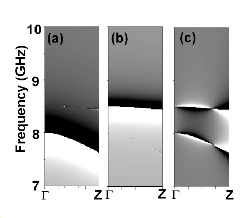
Figure 3: The non-local effective medium from the $\Gamma$ to the Z[001] point for the configuration shown in the caption of Fig. 1: (a) $\epsilon_{T}\left({\rm{\bf q}}\right)$; (b) $\mu_{T}\left({\rm{\bf q}}\right)$ and (c) $\xi\left({\rm{\bf q}}\right)$. White color denotes positive and black color denotes negative values.

For the current configuration, the effect of $\gamma_{12}\left({\rm{\bf q}}\right)$ is rather weak. However, it can become more prominent in other cases. As an example, for the same CsCl lattice structure, we now consider the wavevector ${\rm{\bf q}}$ along the $\Gamma$ to R[111] direction and the particles are now orientated so that the uniaxial electric particle can be polarized along the [-112] direction while the uniaxial magnetic particle can be polarized along the [1-10] direction. This second configuration is shown in Fig. 4. $\epsilon_{T}\left({\rm{\bf q}}\right)$, $\mu_{T}\left({\rm{\bf q}}\right)$ along the $\Gamma$ to R[111] direction are now plotted in Fig. 5 . In Fig. 6(a) and (b), we also plot $\epsilon_{T}\left({\rm{\bf q}}\right)$ and $\mu_{T}\left({\rm{\bf q}}\right)$ against frequency at exactly the R point. From the results, the resonating frequencies depend on ${\rm{\bf q}}$ and both $\epsilon_{T}\left({\rm{\bf q}}\right)$ and $\mu_{T}\left({\rm{\bf q}}\right)$ now clearly diverge at two separate frequencies (instead of one) for every non-zero ${\rm{\bf q}}$ due to the appearance of the term $\gamma_{12}\left({\rm{\bf q}}\right)$. The two resonating frequencies $\omega_{1}\left({\rm{\bf q}}\right)$ (the lower one) and $\omega_{2}\left({\rm{\bf q}}\right)$ (the upper one) can be obtained from Eq. (23) and are governed by

$$\begin{split}\left({\frac{1}{\epsilon_{T}-1}-\Delta\beta_{T}\left({\rm{\bf q}}\right)}\right)\left({\frac{1}{\mu_{T}-1}-\Delta\beta_{T}\left({\rm{\bf q}}\right)}\right)\\ -\left|{\gamma_{12}\left({\rm{\bf q}}\right)}\right|^{2}=0.\end{split}$$ (25)

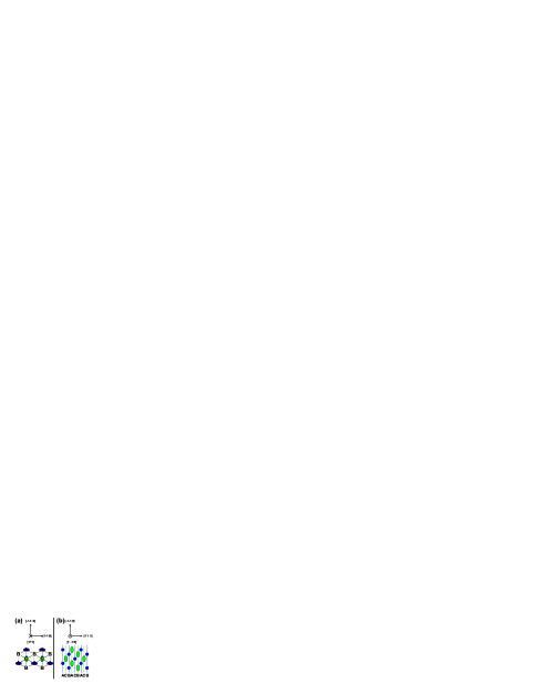
Figure 4: (Color online)A double-lattice configuration specified by Eq. (19) with $\omega_{e}/\left({2\pi}\right)=8GHz$, $A=0.89$, $\omega_{m}/\left({2\pi}\right)=8.5GHz$, $B=0.128$, $\Gamma_{e}=\Gamma_{m}=0$ and lattice constant a= 5 mm. The underlying CsCl structure is viewed along the (a) [111] and (b) [0-10] direction. The uniaxial electric particle (green color) can be polarized along the [-112] direction. The uniaxial magnetic particle (blue color) can be polarized along the [1-10] direction.

Figure 5: The non-local effective medium from the $\Gamma$ to the R point for the configuration shown in the caption of Fig. 4: (a) $\epsilon_{T}\left({\rm{\bf q}}\right)$; (b) $\mu_{T}\left({\rm{\bf q}}\right)$ and (c) $\xi\left({\rm{\bf q}}\right)$. White color denotes positive and black color denotes negative values.

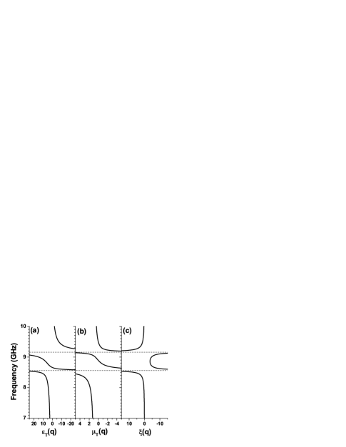
Figure 6: The non-local effective medium at the R point for the configuration shown in the caption of Fig. 4: (a) $\epsilon_{T}\left({\rm{\bf q}}\right)$; (b) $\mu_{T}\left({\rm{\bf q}}\right)$ and (c) $\xi\left({\rm{\bf q}}\right)$.

If the magnetic resonance and the electric resonance are far apart in frequency or the term $\gamma_{12}\left({\rm{\bf q}}\right)$ can be neglected, it decouples to

$$\frac{1}{\epsilon_{T}-1}-\Delta\beta_{T}\left({\rm{\bf q}}\right)=0,$$ (26)

which determines the electric resonating frequency and

$$\frac{1}{\mu_{T}-1}-\Delta\beta_{T}\left({\rm{\bf q}}\right)=0,$$ (27)

which determines the magnetic resonating frequency. It gives us two separate “bands” of resonating frequencies. The term $\Delta\beta_{T}\left({\rm{\bf q}}\right)$ gives us the ${\rm{\bf q}}$ dependence of the electric or the magnetic resonating frequency (shown in the previous example in Fig. 3). However, in the current example, these two bands hybridize with each other so that $\epsilon_{T}\left({\rm{\bf q}}\right)$ or $\mu_{T}\left({\rm{\bf q}}\right)$ has two resonating frequencies instead of one. It is called the cross-coupled resonance here.

Due to the same reason, the $\gamma_{12}\left({\rm{\bf q}}\right)$ term also causes a structure-induced bianisotropy when we bring the electric and magnetic resonances near to each other in frequency. This bianisotropy is induced by the structure instead of the cross-coupling effect of the artificial atoms. The $\xi\left({\rm{\bf q}}\right)$ from the $\Gamma$ to the R point is plotted in Fig. 5(c). It also diverges at $\omega_{1}\left({\rm{\bf q}}\right)$ and $\omega_{2}\left({\rm{\bf q}}\right)$.

We have used a Lorentz-model dispersion (Eq. (19)) for the local effective medium. In fact, $\epsilon_{T}\left({\rm{\bf q}}\right)$, $\mu_{T}\left({\rm{\bf q}}\right)$ and $\xi\left({\rm{\bf q}}\right)$ can be numerically fitted very well by extending the same model:

$$\epsilon_{T}\left({\rm{\bf q}}\right)\approx 1-\sum\limits_{j=1}^{2}\frac{A_{j}\left({\rm{\bf q}}\right)\omega_{j}^{2}\left({\rm{\bf q}}\right)}{\omega^{2}-\omega_{j}^{2}\left({\rm{\bf q}}\right)+i\omega\Gamma_{j}\left({\rm{\bf q}}\right)},$$ (28)

$$\mu_{T}\left({\rm{\bf q}}\right)\approx 1-\sum\limits_{j=1}^{2}\frac{B_{j}\left({\rm{\bf q}}\right)\omega^{2}}{\omega^{2}-\omega_{j}^{2}\left({\rm{\bf q}}\right)+i\omega\Gamma_{j}\left({\rm{\bf q}}\right)},$$ (29)

and

$$\xi\left({\rm{\bf q}}\right)\approx C\left({\rm{\bf q}}\right)\omega^{3}\prod\limits_{j=1}^{2}\frac{1}{\omega^{2}-\omega_{j}^{2}\left({\rm{\bf q}}\right)+i\omega\Gamma_{j}\left({\rm{\bf q}}\right)}.$$ (30)

In the current example at the $R$ point, the expressions obtained by setting $\omega_{1}\left({\rm{\bf q}}\right)/\left({2\pi}\right)=8.57GHz$, $\omega_{2}\left({\rm{\bf q}}\right)/\left({2\pi}\right)=9.17GHz$, $A_{1}\left({\rm{\bf q}}\right)=0.13$, $A_{2}\left({\rm{\bf q}}\right)=0.55$, $B_{1}\left({\rm{\bf q}}\right)=0.10$, $B_{2}\left({\rm{\bf q}}\right)=0.03$, $C\left({\rm{\bf q}}\right)2\pi=0.15GHz^{-1}$ and $\Gamma_{1}\left({\rm{\bf q}}\right)=\Gamma_{2}\left({\rm{\bf q}}\right)=0$ can fit the actual results very well. The fitted result has no noticeable differences from the results shown in Fig. 6.

The extended Lorentz-model dispersion is valid even for an absorptive system. Suppose, now we add some absorption to the system by setting $\Gamma_{e}/\left({2\pi}\right)=0.05GHz$ and $\Gamma_{m}/\left({2\pi}\right)=0.02GHz$ in Eq. (19), the resultant non-local effective medium at the $R$ point is shown in Fig. 7 . The non-local effective medium can still be fitted by the extended Lorentz model but with non-zero $\Gamma_{1}\left({\rm{\bf q}}\right)$ and $\Gamma_{2}\left({\rm{\bf q}}\right)$. In this case, we set $\Gamma_{1}\left({\rm{\bf q}}\right)/\left({2\pi}\right)=0.025GHz$ and $\Gamma_{2}\left({\rm{\bf q}}\right)/\left({2\pi}\right)=0.045GHz$ while all other parameters remain the same. The fitted expressions also show no noticeable differences to the results shown in Fig. 7 .

From Fig. 7, we see that the imaginary part of both $\epsilon_{T}\left({\rm{\bf q}}\right)$ and $\mu_{T}\left({\rm{\bf q}}\right)$ are positive. For a bianisotropic medium, there are no general requirements that the imaginary part of the permittivity and the permeability should be positive. However, within the dipolar model, from Eq. (23) with $\beta_{T}\left({\omega,{\rm{\bf q}}}\right)$ being real, it is easy to show that both $\epsilon_{T}\left({\rm{\bf q}}\right)$ and $\mu_{T}\left({\rm{\bf q}}\right)$ have positive imaginary part if the local $\epsilon_{T}$ and $\mu_{T}$ have positive imaginary part, i.e. $\Gamma_{1}\left({\rm{\bf q}}\right)$ and $\Gamma_{2}\left({\rm{\bf q}}\right)$ should be positive. In our approach, we parameterize the effective medium by using ${\rm{\bf q}}$ such that ${\rm{\bf q}}$ is always a real vector within the first Brillouin zone. If, on the other hand, ${\rm{\bf q}}$ is allowed to be complex (e.g. traveling along the dispersion of an eigenmode and becoming complex within the resonance gap where no propagating eigenmodes can be found), a negative imaginary part in $\epsilon_{T}\left({\rm{\bf q}}\right)$ or $\mu_{T}\left({\rm{\bf q}}\right)$ may appear around a cross-coupled resonance. Koschny:2005

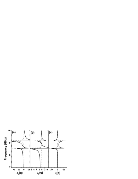
Figure 7: (Color online)The non-local effective medium at the R point for the configuration shown in the caption of Fig. 4 with $\Gamma_{e}=0.05$ and $\Gamma_{m}=0.02$: (a) $\epsilon_{T}\left({\rm{\bf q}}\right)$ ; (b) $\mu_{T}\left({\rm{\bf q}}\right)$; (c) $\xi\left({\rm{\bf q}}\right)$. The blue solid line shows the real part and the gray dashed line shows the imaginary part.

The structure-induced bianisotropy $\xi\left({\rm{\bf q}}\right)$ appears even if the local effective medium does not suffer bianisotropy. $\xi\left({\rm{\bf q}}\right)$ is generally present and it is purely real for a non-absorptive system in our example. It disappears in the local effective medium limit only if the particles do not suffer cross-coupling and the particles are placed in a carefully chosen lattice. For example, if the sublattices of the two types of particles are displaced in the z direction (along ${\rm{\bf q}})$ with respect to each other, the 2D symmetry perpendicular to ${\rm{\bf q}}$ does not change so that the constitutive tensors can still be described by Eq. (24). However, $\xi\left({{\rm{\bf q}}={\rm{\bf 0}}}\right)$ will not vanish and it is a purely imaginary number. On the other hand, if the lattice is not displaced but the particles suffer cross coupling, $\xi\left({{\rm{\bf q}}={\rm{\bf 0}}}\right)$ also does not vanish and it is purely imaginary. Xudong:2005

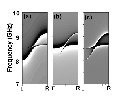
Figure 8: The non-local effective medium from the $\Gamma$ to the R point for the configuration shown in the caption of Fig. 4 with lattice constant a changed to 2.5 mm: (a) $\epsilon_{T}\left({\rm{\bf q}}\right)$; (b) $\mu_{T}\left({\rm{\bf q}}\right)$ and (c) $\xi\left({\rm{\bf q}}\right)$. White color denotes positive and black color denotes negative values.

The structure-induced bianisotropy and cross-coupled resonance are both due to the term $\gamma_{12}\left({\rm{\bf q}}\right)$. In fact, with a smaller lattice constant, the interaction becomes smaller. Fig. 8 shows the $\epsilon_{T}\left({\rm{\bf q}}\right)$, $\mu_{T}\left({\rm{\bf q}}\right)$ and $\xi\left({\rm{\bf q}}\right)$ along the $\Gamma$ to R[111] direction when the lattice constant $a$ is changed a smaller value 2.5 mm. The splitting between the two resonating frequencies is smaller than in Fig. 5. On the other hand, if the lattice constant becomes larger, the term $\gamma_{12}\left({\rm{\bf q}}\right)$ cannot be neglected in finding the effective medium or in finding the dispersion.

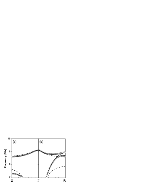
Figure 9: Dispersion diagram (open circles) for the configuration shown in (a) Fig. 1 along the $\Gamma Z$ direction and the configuration shown in (b) Fig. 4 along the $\Gamma R$ direction. The black dashed line represents the corresponding dispersion obtained from the local effective medium. The blue solid line represents the perturbed dispersion from the local one.

We have investigated the constitutive tensors of the metamaterial. After finding the effective medium, the dispersion diagram can also be found. The dispersion relation of the effective medium is governed by

$$\det\left({\left\langle{T}\right\rangle^{-1}\left({\rm{\bf q}}\right)}\right)=0.$$ (31)

After some algebra, we have

$$\begin{split}\det\left({\left\langle{{T}^{-1}}\right\rangle\left({\rm{\bf q}}\right)}\right)&=\frac{1}{q^{2}-k_{0}^{2}}\\ &\times\frac{\left|{q+k_{0}\xi\left({\rm{\bf q}}\right)}\right|^{2}-k_{0}^{2}\epsilon_{T}\left({\rm{\bf q}}\right)\mu_{T}\left({\rm{\bf q}}\right)}{\left({\epsilon_{T}\left({\rm{\bf q}}\right)-1}\right)\left({\mu_{T}\left({\rm{\bf q}}\right)-1}\right)-\left|{\xi\left({\rm{\bf q}}\right)}\right|^{2}}\end{split}$$ (32)

and the dispersion relation is therefore

$$\left|{q+k_{0}\xi\left({\rm{\bf q}}\right)}\right|^{2}=k_{0}^{2}\epsilon_{T}\left({\rm{\bf q}}\right)\mu_{T}\left({\rm{\bf q}}\right).$$ (33)

There is an extra term $k_{0}\xi\left({\rm{\bf q}}\right)$ in the dispersion relation comparing to the one obtained from the local effective medium: $q^{2}=k_{0}^{2}\epsilon_{T}\mu_{T}.$ Unlike the case of the local effective medium which serves as an approximation of the actual band structure, the dispersion relation shown in Eq. (33) can be used to find the band structure which shows no noticeable differences to the actual band structure if we solve it directly without first finding the non-local effective medium. For band structure of a single lattice consisting artificial particles of only electric or only magnetic response, see Ref. Belov:2005, and Ref. Kempa:2005, .

The dispersion diagram along the direction $\Gamma Z$ for the first configuration (Fig. 1) and the dispersion diagram along the direction $\Gamma R$ for the second configuration (Fig. 4) are shown in Fig. 9(a) and (b) respectively. They are plotted in open black circles while the dispersion diagram obtained from the local effective medium is plotted in dashed line. Along the $\Gamma Z$ direction for the first configuration, they look very similar especially near the Brillouin zone center. In fact, the formation of the non-local bands can be understood from a perturbation point of view by assuming small $\Delta\beta_{T}\left({\rm{\bf q}}\right)$ and $\gamma_{12}\left({\rm{\bf q}}\right)$. For a fixed ${\rm{\bf q}}$, we can approximate the change in square frequency from the local to the non-local dispersion by

$$\begin{split}\frac{\partial k_{0}^{2}\epsilon_{T}\mu_{T}}{\partial k_{0}^{2}}\Delta k_{0}^{2}&=\left({\epsilon_{T}-1}\right)\left({\mu_{T}-1}\right)\left({q^{2}-k_{0}^{2}}\right)\\ &\times\det\left({\left\langle{T}\right\rangle^{-1}\left({\rm{\bf q}}\right)}\right),\end{split}$$ (34)

which is evaluated along one of the bands obtained from the local effective medium. (The proof is not shown here.) By substituting Eq. (23) into it and neglect the second order effect of $\beta_{T}\left({\rm{\bf q}}\right)$ and $\gamma\left({\rm{\bf q}}\right)$, we have

$$\begin{split}\frac{d\omega^{2}\epsilon_{T}\mu_{T}}{d\omega^{2}}\frac{\Delta\omega^{2}}{\omega^{2}}&\approx-\beta_{T}\left({\rm{\bf q}}\right)\left({\mu_{T}\left({\epsilon_{T}-1}\right)^{2}+\epsilon_{T}\left({\mu_{T}-1}\right)^{2}}\right)\\ &+Re\left({\gamma_{12}\left({\rm{\bf q}}\right)}\right)2\sqrt{\epsilon_{T}\mu_{T}}\left({\epsilon_{T}-1}\right)\left({\mu_{T}-1}\right).\end{split}$$ (35)

This perturbed dispersion is plotted in Fig. 9 in solid line. We can see that it approximates the actual non-local dispersion very well in the $\Gamma$Z direction of the first configuration. In the $\Gamma$R direction, the first band (having positive refractive index in the local limit) and the second band (having negative refractive index in the local limit) hybridize with each other to form the actual band.

For every mode in the dispersion diagram, we can characterize it by defining the refractive index $n$ of the mode using $q^{2}=n^{2}k_{0}^{2}$ and defining its characteristic impedance Z to be the ratio between the tangential $E$ and the tangential $H$ field. They are governed by

$$\begin{split}n/Z&=\frac{\epsilon_{T}\left({\rm{\bf q}}\right)}{1+\xi\left({\rm{\bf q}}\right)k_{0}/q},\\ nZ&=\frac{\mu_{T}\left({\rm{\bf q}}\right)}{1+\xi\left({\rm{\bf q}}\right)k_{0}/q}.\\ \end{split}$$ (36)

For example, the $n$ and $Z$ along the band in the $\Gamma$Z direction in Fig. 9 are plotted as solid lines in Fig. 10 for the double-negative band. The corresponding values for the local effective medium ($n^{2}=\epsilon_{T}\mu_{T}$,$Z=\sqrt{\mu_{T}/\epsilon_{T}})$ are also shown in dashed lines in the same figure. We can see that the local effective medium works very well for the propagating bands unless it is near the Brillouin zone edge and near the resonance gap.

Figure 10: Solid line: characteristic impedance and the refractive index of the double-negative band in the $\Gamma Z$ direction. Dashed line: corresponding values for the local medium.

We have examined the non-local effective medium governing the transverse waves. In fact, if the artificial particles are oriented so that they can only be polarized in a single direction along the z-axis, the metamaterial supports longitudinal waves whose propagating direction is also along the z-axis. We can do the similar analysis to obtain the longitudinal permittivity $\epsilon_{L}({\bf q})$ and the longitudinal permeability $\mu_{L}({\bf q})$. In this case, the electric and magnetic response are decoupled, $\epsilon_{L}({\bf q})$ and $\mu_{L}({\bf q})$ can also be fitted by using a Lorentz-model dispersion:

$$\epsilon_{L}\left({\rm{\bf q}}\right)\approx 1-\frac{A_{e}\left({\rm{\bf q}}\right)\omega_{e}^{2}\left({\rm{\bf q}}\right)}{\omega^{2}-\omega_{e}^{2}\left({\rm{\bf q}}\right)+i\omega\Gamma_{e}\left({\rm{\bf q}}\right)},$$ (37)

and

$$\mu_{L}\left({\rm{\bf q}}\right)\approx 1-\frac{B_{m}\left({\rm{\bf q}}\right)\omega^{2}}{\omega^{2}-\omega_{m}^{2}\left({\rm{\bf q}}\right)+i\omega\Gamma_{m}\left({\rm{\bf q}}\right)},$$ (38)

The electric longitudinal mode (or the electric bulk plasmon with macroscopic E field along ${\bf q}$) has a dispersion relation governed by

$$\epsilon_{L}(\bf{q})=0,$$ (39)

and the dispersion relation for the the magnetic longitudinal mode (or the magnetic bulk plasmon with macroscopic H field along ${\bf q}$) is governed by

$$\mu_{L}(\bf{q})=0.$$ (40)

With spatial dispersion such that $\epsilon_{L}(\bf{q})$ and $\mu_{L}(\bf{q})$ depends on ${\bf q}$, the band for either the electric or magnetic longitudinal mode becomes dispersive to form a narrow band instead of a flat line in the local medium picture.

V Conclusion

We have established a numerical method based on a dipolar model to obtain the non-local effective medium of a metamaterial. In particular, we have concentrated on the double lattice structure in which one sublattice holds the electric artificial atoms and another sublattice holds the magnetic artificial atoms. Once the dipolar scattering properties of the atoms or the local effective medium parameters are specified, the non-local effective medium with all the four constitutive tensors can be obtained on the whole frequency regime including frequencies near the resonance gap. We found that the metamaterial should be regarded as bianisotropic near the resonance gap even if the artificial atoms do not suffer cross-coupling. In this case, the cross-coupling comes from spatial dispersion and it also induces a cross-coupled resonance for metamaterials having both electric and magnetic resonances. Within our model, the cross-coupled resonance can still be understood using a Lorentz dispersion model. The effect of the cross-coupling from spatial dispersion depends on the microstructure and it is larger at a higher normalized frequency (or a larger lattice constant).

VI Acknowledgment

This work is supported by the Croucher Foundation fellowship from Hong Kong.

Appendix A The Green’s Tensor

The radiation field from an electric dipole ${\rm{\bf p}}$ together with a magnetic dipole ${\rm{\bf m}}$ at the origin in the vacuum is

$$\left[{{\begin{array}[]{*{20}c}{{\rm{\bf E}}\left({\rm{\bf r}}\right)/\eta_{0}\hfill}\\ {{\rm{\bf H}}\left({\rm{\bf r}}\right)\hfill}\\ \end{array}}}\right]={G}_{0}\left({\rm{\bf r}}\right)\cdot\left[{{\begin{array}[]{*{20}c}{c_{0}{\rm{\bf p\hfill}}}\\ {\rm{\bf m\hfill}}\\ \end{array}}}\right],$$ (41)

where the ${G}_{0}$ matrix is defined by

$${G}_{0}\left({\rm{\bf r}}\right)=\left[{{\begin{array}[]{*{20}c}{k_{0}^{2}\mathord{\buildrel\lower 3.0pt\hbox{$\scriptscriptstyle\leftrightarrow$}\over{G}}_{0}\left({\rm{\bf r}}\right)\hfill}&{ik_{0}\nabla\times\mathord{\buildrel\lower 3.0pt\hbox{$\scriptscriptstyle\leftrightarrow$}\over{G}}_{0}\left({\rm{\bf r}}\right)\hfill}\\ {-ik_{0}\nabla\times\mathord{\buildrel\lower 3.0pt\hbox{$\scriptscriptstyle\leftrightarrow$}\over{G}}_{0}\left({\rm{\bf r}}\right)\hfill}&{k_{0}^{2}\mathord{\buildrel\lower 3.0pt\hbox{$\scriptscriptstyle\leftrightarrow$}\over{G}}_{0}\left({\rm{\bf r}}\right)\hfill}\\ \end{array}}}\right],$$ (42)

with the vacuum Green’s tensor $\mathord{\buildrel\lower 3.0pt\hbox{$\scriptscriptstyle\leftrightarrow$}\over{G}}_{0}$ defined by

$$\mathord{\buildrel\lower 3.0pt\hbox{$\scriptscriptstyle\leftrightarrow$}\over{G}}_{0}\left({\rm{\bf r}}\right)=\left({\mathord{\buildrel\lower 3.0pt\hbox{$\scriptscriptstyle\leftrightarrow$}\over{I}}+\frac{1}{k_{0}^{2}}\nabla\nabla}\right)\frac{\exp\left({ik_{0}r}\right)}{4\pi r},$$ (43)

where $\mathord{\buildrel\lower 3.0pt\hbox{$\scriptscriptstyle\leftrightarrow$}\over{I}}$ is the 3-by-3 identity tensor.

The Fourier Transform of ${G}_{0}\left({\rm{\bf r}}\right)$ is given by

$$\begin{split}{G}_{0}\left({\rm{\bf q}}\right)&=\int{{G}_{0}\left({\rm{\bf r}}\right)\exp\left({-i{\rm{\bf q}}\cdot{\rm{\bf r}}}\right)d^{3}r}\\ &=\left[{{\begin{array}[]{*{20}c}{k_{0}^{2}\mathord{\buildrel\lower 3.0pt\hbox{$\scriptscriptstyle\leftrightarrow$}\over{G}}_{0}\left({\rm{\bf q}}\right)\hfill}&{-k_{0}{\rm{\bf q}}\times\mathord{\buildrel\lower 3.0pt\hbox{$\scriptscriptstyle\leftrightarrow$}\over{G}}_{0}\left({\rm{\bf q}}\right)\hfill}\\ {k_{0}{\rm{\bf q}}\times\mathord{\buildrel\lower 3.0pt\hbox{$\scriptscriptstyle\leftrightarrow$}\over{G}}_{0}\left({\rm{\bf q}}\right)\hfill}&{k_{0}^{2}\mathord{\buildrel\lower 3.0pt\hbox{$\scriptscriptstyle\leftrightarrow$}\over{G}}_{0}\left({\rm{\bf q}}\right)\hfill}\\ \end{array}}}\right],\\ \end{split}$$ (44)

where

$$\mathord{\buildrel\lower 3.0pt\hbox{$\scriptscriptstyle\leftrightarrow$}\over{G}}_{0}\left({\rm{\bf q}}\right)=\frac{1}{q^{2}-k_{0}^{2}}\left({\mathord{\buildrel\lower 3.0pt\hbox{$\scriptscriptstyle\leftrightarrow$}\over{I}}-\hat{q}\hat{q}}\right)-\frac{1}{k_{0}^{2}}\hat{q}\hat{q}.$$ (45)

Appendix B Restriction on the scattering phase shift of a single particle

Here, we will consider the restriction on the polarizability for a lossless classical uniaxial particle which can be described by its permittivity distribution $\epsilon_{s}\left({\rm{\bf r}}\right)$ and its permeability distribution $\mu_{s}\left({\rm{\bf r}}\right)$. The particle has a finite radius $r_{s}$ such that it is vacuum outside the sphere of radius $r_{s}$ centered at the origin. Without losing generality, we consider the situation that “m” wave (with angular momentum $l=1$ and $m=0)$ is scattered from the particle which can be magnetically polarized along the z-direction but not the other directions. We also assume that the particle has no cross-coupling, i.e. the electric dipole moment is zero when the local electric field is zero here. The total wave outside the particle can be written in the following form:

$${\rm{\bf E}}=\frac{u\left(k_{0}r\right)}{r}{\rm{\bf r}}\times\nabla Y_{l=1,m=0}\left(\hat{r}\right)$$ (46)

where

$$u\left(\theta\right)=\frac{\theta}{2}\left({h_{1}^{\ast}\left(\theta\right)+\exp\left({2i\delta_{1}^{\left(m\right)}}\right)h_{1}\left(\theta\right)}\right),$$ (47)

with $h_{l}\left(\theta\right)$ being the out-going spherical Hankel function, and $Y_{lm}\left(\hat{r}\right)$ being the spherical harmonic. $\delta_{l}^{\left(m\right)}$, the phase shift in scattering, is a real number for a lossless particle and it is related to the magnetic polarizability through

$$\frac{ik_{0}^{3}\alpha_{m}}{3\pi}=\exp\left({2i\delta_{1}^{\left(m\right)}}\right)-1.$$ (48)

On the other hand, from the Maxwell equations, we can prove the following identity

$$\begin{split}\frac{1}{4}\int{\epsilon_{0}\frac{\partial\omega\epsilon\left({\rm{\bf r}}\right)}{\partial\omega}\left|{\rm{\bf E}}\right|^{2}+\mu_{0}\frac{\partial\omega\mu\left({\rm{\bf r}}\right)}{\partial\omega}\left|{\rm{\bf H}}\right|^{2}d^{3}r}=\\ -\frac{i}{4}\oint{\left({\frac{\partial{\rm{\bf E}}}{\partial\omega}\times{\rm{\bf H}}^{\ast}+{\rm{\bf E}}^{\ast}\times\frac{\partial{\rm{\bf H}}}{\partial\omega}}\right)\cdot d{\rm{\bf A}}}.\end{split}$$ (49)

The volume and the surface integrals are taken to be the volume and the surface of the sphere of radius $r_{s}$ which encloses the particle completely. By substituting Eq. (46) into Eq. (49), we obtain

$$\begin{split}\frac{1}{4}\int{\epsilon_{0}\frac{\partial\omega\epsilon\left({\rm{\bf r}}\right)}{\partial\omega}\left|{\rm{\bf E}}\right|^{2}+\mu_{0}\frac{\partial\omega\mu\left({\rm{\bf r}}\right)}{\partial\omega}\left|{\rm{\bf H}}\right|^{2}d^{3}r}=\\ \frac{1}{4\omega^{2}\mu_{0}}\left({{u}^{\prime\ast}\left(\theta\right)\frac{\partial u\left(\theta\right)}{\partial\omega}-\frac{\partial{u}^{\prime}\left(\theta\right)}{\partial\omega}u^{\ast}\left(\theta\right)}\right),\end{split}$$ (50)

where $\theta=\omega r_{s}/c$. Finally, we recognize the l.h.s. of Eq. (50) is just the time-averaged total electromagnetic energy ($\mathscr{E})$ within the sphere for a narrow band signal centered at the angular frequency $\omega$. By substituting Eq. (47) into Eq. (50), we can express the time-averaged total energy in terms of $\delta_{l}^{\left(m\right)}$:

$$\begin{split}\omega^{3}\mathscr{E}\propto&\omega\frac{d\delta_{1}^{\left(m\right)}}{d\omega}-\frac{1}{2\theta^{3}}(1+2\theta^{2}-2\theta^{4}-\cos 2\left({\theta+\delta_{1}^{\left(m\right)}}\right)\\ &-2\theta\sin 2\left({\theta+\delta_{1}^{\left(m\right)}}\right)),\end{split}$$ (51)

which must be a positive number. The derivation for the electric scattering phase shift is similar. Moreover, the derivation also applies for an isotropic particle instead of an uniaxial particle being discussed here.

References

(1) D. R. Smith, D. C. Vier, Th. Koschny, and C. M. Soukoulis, Phys. Rev. E71, 036617 (2005).
(2) J. B. Pendry, A. J. Holden, D. J. Robbins, and W. J. Stewart, IEEE Trans. Microwave Theory Tech.47, 2075 (1999).
(3) D. R. Smith, J. Gollub, J. J. Mock, W. J. Padilla and D. Schurig , J. Appl. Phys.100, 024507 (2006).
(4) J.-M. Lerat, N. Malléjac, and O. Acher, J. Appl. Phys.100, 084908 (2006).
(5) P. A. Belov and C. R. Simovski, Phys. Rev. B73, 045102 (2006).
(6) P. A. Belov, R. Marques, S. I. Maslovski, I. S. Nefedov, M. Silveirinha, C. R. Simovski, and S. A. Tretyakov, Phys. Rev. B67 113103 (2003).
(7) M. G. Silveirinha, Phys. Rev. E73, 046612 (2006).
(8) M. A. Shapiro, G. Shvets, J. R. Sirigiri and R. J. Temkin, Opt. Lett.31, 2051 (2006).
(9) F. J. García de Abajo and J. J. Sáenz, Phys. Rev. Lett. 95, 233901 (2005).
(10) R. Marques, F. Medina, and R. Rafii-El-Idrissi, Phys. Rev. B65, 144440 (2002).
(11) Xudong Chen, Bae-Ian Wu, Jin Au Kong, and Tomasz M. Grzegorczyk , Phys. Rev. E71, 046610 (2005).
(12) D. Schurig, J. J. Mock, and D. R. Smith, Appl. Phys. Lett.88 041109 (2006).
(13) V. Dmitriev, Prog. Electromagn. Res.28, 43 (2000).
(14) S. Ponti, C. Oldano, and M. Becchi, Phys. Rev. E64, 021704 (2001).
(15) S. Ponti, J. A. Reyes and C. Oldano, J. Phys.: Cond. Matter14, 10173 (2002).
(16) Juan D. Baena, Ricardo Marqués, Francisco Medina, and Jesús Martel, Phys. Rev. B69 014402 (2004).
(17) P. A. Belov, and C. R. Simovski, Phys. Rev. E72, 026615 (2005).
(18) S. A. Tretyakov, IEEE Trans. Antennas Propag.51 2652 (2003).
(19) G. D. Mahan, Phys. Rev. B74, 033407 (2006).
(20) A. D. Boardman and K. Marinov, Phys. Rev. B73, 165110 (2006).
(21) S. Tretyakov, Analytical Modeling in Applied Electromagnetics (Artech House, Boston 2003).