We apply a meron cluster algorithm to the XY spin chain, which describes a quantum rotor. This is a multi-cluster simulation supplemented by an improved estimator, which deals with objects of half-integer topological charge. This method is powerful enough to provide precise results for the model with a $\theta$-term — it is therefore one of the rare examples, where a system with a complex action can be solved numerically. In particular we measure the correlation length, as well as the topological and magnetic susceptibility. We discuss the algorithmic efficiency in view of the critical slowing down. Due to the excellent performance that we observe, it is strongly motivated to work on new applications of meron cluster algorithms in higher dimensions.

1 Introduction

The functional integral formalism of quantum physics deals with infinite dimensional integrals, which can only be computed explicitly in a few simple situations. A non-perturbative method to tackle models, which are not analytically soluble, starts by a regularisation to a finite number of degrees of freedom. This is usually achieved by a lattice discretisation of the time (in quantum mechanics) or of the space-time (in quantum field theory). In a finite volume the functional integral is then given by a finite set of single variable integrals. One tries to compute them numerically and — based on a variety of such results — to extrapolate to the continuum and to infinite volume. The transition to Euclidean time is very helpful to speed up the convergence of the integrals.

However, the number of integrals still tends to be so large that straight numerical integration is hopeless. Instead one performs Monte Carlo simulations to generate a set of paths or field configurations with the Boltzmann probability distribution given by the Euclidean action. Thus one evaluates the expectation values of the observables of interest directly at finite interaction strength (in contrast to perturbation theory). On the other hand, one has to face errors due to the limited statistics and uncertainties in the extrapolations.

Hence it is essential to optimise the algorithmic tools for such simulations. The Metropolis algorithm is the most established procedure, but in many cases it is far from optimal. It can be refined to cluster algorithms [2, 3] which are by far more efficient for some set of models (for a review, see Ref. [4]). Unfortunately this set, where it could be applied successfully, is still quite small — in particular it excludes gauge theories up to now. But in the light of the striking success in specific spin models, it is highly motivated to explore cluster algorithms further. Here we present successful tests on (classical) spin chains, which describe quantum mechanical systems.

Unlike the Metropolis algorithm, cluster algorithms do not proceed from one configuration to the next by updating single spins, but by flipping whole clusters of them. First, this is promising in view of the thermalisation time needed in the beginning of a simulation. Later one expects to generate with the cluster algorithm well de-correlated configurations (which are needed for the measurements) with a modest number of simulation steps. In addition, multi-cluster algorithms can often be combined with an “improved estimator”, which allows for the inclusion of lots of configurations that do not need to be Monte Carlo generated explicitly. All these properties help to reduce the computer time required to measure an observable numerically to a given accuracy. This will be clearly confirmed for the system under consideration in this work, in particular as one approaches the continuum limit.

We apply this technique to the $O(2)$ spin chain (the XY model), to be described in Section 2. There is a neat way to attach a half-integer topological charge to each cluster. This is the basis of a meron cluster simulation, which was first applied to a 2d $O(3)$ model on a triangular lattice (with a constrained maximal angle between neighbouring spins) [10], see also Ref. [11]. In this framework an improved estimator is extremely powerful. Variants of the meron cluster algorithm can also handle fermionic spin models successfully [12].

In Sections 3 and 4 we present a novel application of this algorithm [13]. It enables us to approach the continuum limit much better than the Metropolis algorithm, and to suppress the notorious “critical slowing down”. As in the original application, it is powerful enough to even explore the system with a $\theta$-term. In almost all cases the simulation of a system with a complex Euclidean action is hardly feasible so far (perhaps up to a region of very small imaginary parts). Here we present one of the rare exceptions. Moreover, the constraint on the angles is not necessary in our case; the latter was required for technical reasons in the original application [10] (though it did not affect the universality class). Section 5 is dedicated to our conclusions and an outlook on potential applications of the techniques discussed here to a system of light quarks at high temperature.

2 The quantum rotor

We deal with a free scalar particle of mass $m$ on a circle of radius $1$, i.e. a quantum rotor. Its position is given by an angle $\varphi(t)$, where $t$ is the Euclidean time, so the Lagrangian reads ${\bf L}=\frac{m}{2}\dot{\varphi}(t)^{2}$. We consider the propagator $G$ between the end-points $\varphi(0)=0$ and $\varphi(T)=0$ $(T>0)$, i.e. we assume periodic boundary conditions. In the path integral formulation it can be decomposed into disjoint contributions with different winding numbers $\nu$. It is therefore the simplest quantum system with topological sectors. As in QCD we can also insert a $\theta$-term in this summation, which leads to

$$G(0,T;0,0) = \sum_{\nu=-\infty}^{+\infty}G_{\nu}(0,T;0,0)\,e^{i\nu\theta}$$ (2.1)

$$= \sqrt{\frac{m}{2\pi T}}\sum_{\nu=-\infty}^{\infty}\exp\Big{[}-\frac{2m\pi^{2}}{T}\nu^{2}+i\nu\theta\Big{]}$$

$$= \frac{1}{2\pi}\sum_{\nu=-\infty}^{\infty}\exp\Big{[}-\frac{T}{2m}\Big{(}\nu-\frac{\theta}{2\pi}\Big{)}^{2}\Big{]}\ .$$

$G_{\nu}$ is the free propagator $\langle 2\pi\nu,T|0,0\rangle$ on a line, and we set $\hbar=1$. It is sufficient to consider $\theta\in[0,\pi]$.

In QCD it appears natural that a $\theta$-term should occur, hence it is a mystery — known as the “strong CP problem” — why the observed $\theta$-angle is zero (or very close to it). In our case, a finite $\theta$-angle does describe a physical situation, if we assume the particle to carry an electric charge $q$ and a magnetic flux $\Phi$ to cross the circle. Then we identify $\theta=2\pi q\Phi$ (Aharonov-Bohm effect). Unlike QCD, we can evaluate in the present toy model the effect of $\theta>0$ precisely, see Section 4.

We now discretise the period $T$ in $L$ equal steps. We use lattice units, i.e. we set the step length $T/L=1$. We denote $\varphi(t=j)=\varphi_{j}$, and periodicity implies $\varphi_{j+L}\equiv\varphi_{j}$. The standard action on this temporal lattice reads

$$S_{s}[\varphi]=m\sum_{j=1}^{L}\ [1-\cos(\varphi_{j+1}-\varphi_{j})]\ .$$ (2.2)

In contrast, the perfect lattice action [15], which is obtained from an infinite iteration of renormalisation group transformations, distinguishes the topological sector that the particle may enter at time slice $j$

$$S_{p}[\varphi,\nu]=\frac{m}{2}\sum_{j=1}^{L}\ [\varphi_{j+1}-\varphi_{j}+2\pi\nu_{j}]^{2}\ .$$ (2.3)

In the functional integral all these sectors $\nu_{j}\in Z\!\!\!Z$ are summed over, which reproduces the exact continuum result.

This discrete system has another interpretation as a spin chain. On each site $j$ a classical spin $\vec{S}_{j}=(S^{(1)}_{j},S^{(2)}_{j})$ of length $\vec{S}_{j}^{\,2}=1$ is attached. This is the XY model, which has a global $O(2)$ symmetry. If we stay with periodic boundary conditions and assume only nearest neighbour interactions with some coupling $c$, we arrive at the partition function

$$Z={\rm Tr}\,e^{-\beta H[\vec{S}]}\ ,\qquad H[\vec{S}]=-c\sum_{j=1}^{L}\vec{S}_{j+1}\cdot\vec{S}_{j}\ .$$ (2.4)

The trace means the sum over all spin configurations $[\vec{S}]=(\vec{S}_{1},\vec{S}_{2},\dots,\vec{S}_{L})$, and $\beta$ is an inverse temperature. If we identify the constants as $\beta c=m$, we obtain the standard lattice path integral of the quantum rotor at $\theta=0$ (up to an additive constant in the action); the angle $\varphi_{j}$ describes the direction of the spin $\vec{S}_{j}$, and also the spin model can be generalised by a $\theta$-term.

The standard discretised system does not have natural topological sectors, because all configurations can be continuously deformed into one another (in contrast to the case of continuous time). Still one often introduces topologies, which is, however, ambiguous. The most obvious option is the geometric charge [17], which can be formulated analogously for instance in $N$-dimensional $O(N+1)$ models, or in 4d Yang-Mills gauge theories [18]. In our case, the geometric charge amounts to

$$\nu^{\rm(g)}=\frac{1}{2\pi}\sum_{j=1}^{L}\Delta\varphi_{j}\in Z\!\!\!Z\ ,$$ (2.5)

where $\Delta\varphi_{j}=(\varphi_{j+1}-\varphi_{j})\in(-\pi,\pi]$.

We will also consider alternative formulations.

2.1 Observables

We are going to extract the correlation length $\xi$ as usual from the exponential decay of the connected 2-point function (resp. a cosh function due to the periodic boundary conditions). $\xi$ sets the scale of the system, and physically sensible results usually require

$$1\ll\xi\ll L\ .$$ (2.6)

The first (second) inequality implies that discretisation artifacts (finite size effects) are harmless.

Our observables are the topological and the magnetic susceptibility,

$$\chi_{t} = \frac{1}{L}\Big{(}\langle\nu^{2}\rangle-\langle\nu\rangle^{2}\Big{)}\ ,$$ (2.7)

$$\chi_{m} = \frac{1}{L}\Big{(}\langle\vec{M}^{2}\rangle-\langle\vec{M}\rangle^{2}\Big{)}\ ,\quad\vec{M}=\sum_{j=1}^{L}\vec{S}_{j}\ .$$ (2.8)

Let us assume the cosh shape of the correlation functions to hold at all distances. Then $\chi_{m}$ can be computed as follows,

$$\chi_{m} = \frac{1}{L}\Big{\langle}\ \Big{(}\sum_{j=1}^{L}\vec{S}_{j}\Big{)}^{2}\Big{\rangle}=1+\sum_{j=2}^{L}\langle\vec{S}_{1}\vec{S}_{j}\rangle$$ (2.9)

$$\simeq 1+\sum_{j=2}^{L}\Big{[}e^{-(j-1)/\xi}+e^{-(L+1-j)/\xi}\Big{]}=2\ \frac{1-e^{-L/\xi}}{1-e^{-1/\xi}}-1\ .$$

We now assume in addition the inequalities (2.6) to hold. In fact our simulations — to be presented below — were performed consistently at $L/\xi\approx 20$. Thus the term $e^{-L/\xi}$ can be safely neglected, which leads to

$$\frac{\chi_{m}}{\xi}\simeq 2+\frac{1}{6\xi^{2}}+O(\xi^{-3})\ .$$ (2.10)

3 A meron cluster simulation of the XY model

3.1 The algorithm

We start by briefly reviewing the multi-cluster algorithm for $O(N)$ models [3, 19], and in particular its extension to a meron cluster algorithm [10].

A step of the multi-cluster algorithm begins by building clusters, which are sets of neighbouring spins. To this end, a random direction $\vec{r}$ is chosen in an isotropic way ($|\vec{r}|=1$), and each spin $\vec{S}_{j}$ is split into $\vec{S}_{j}^{\parallel}=(\vec{S}_{j}\cdot\vec{r})\,\vec{r}$ and $\vec{S}_{j}^{\perp}=\vec{S}_{j}-\vec{S}_{j}^{\parallel}$. A virtual bond is set between the sites $j$ and $j+1$ with the probability

$$p_{j}=\left\{\begin{array}[]{ll}1-e^{-2\beta\vec{S}_{j}^{\parallel}\vec{S}_{j+1}^{\parallel}}&\textnormal{\quad if \quad}\vec{S}_{j}^{\parallel}\cdot\vec{S}_{j+1}^{\parallel}>0\\ 0&\textnormal{\quad otherwise \ .}\end{array}\right.$$ (3.1)

Then a cluster is composed of neighbouring spins connected by bonds; it may also consist of a single spin, if the latter is disconnected. A step of the algorithm ends with “flipping” each cluster with the probability $1/2$ [2]. Flipping a cluster means that all its spins are mirrored at the plane perpendicular to $\vec{r}$, $\quad\vec{S}_{j}^{\parallel}\rightarrow-\vec{S}_{j}^{\parallel},\quad\vec{S}_{j}^{\perp}\rightarrow\vec{S}_{j}^{\perp}$. This algorithm respects ergodicity and detailed balance [3].

Let us numerate the clusters with $c=1,2,\dots$. A topological charge $Q_{c}$ can be assigned to each cluster based on the difference of the total topological charge $\nu$ (i.e. the winding number) of the chain when the cluster is in its initial orientation, and after it has been flipped [10],

$$Q_{c}=\frac{\nu_{c{\rm-initial}}-\nu_{c{\rm-flipped}}}{2}\ .$$ (3.2)

On the right-hand-side we use the geometric charge (2.5). $Q_{c}$ is a half-integer, which remains unchanged if any other clusters are flipped, so it is determined locally [13]. To illustrate this important property, let $\vec{S}_{j}$ …$\vec{S}_{k}$ be the spins of a specific cluster. We denote the sum of the relative angles $\Delta\varphi_{j}\in(-\pi,\pi]$ (cf. eq. (2.5)) between the successive neighbouring spins $l$ to $n$ as $\widehat{\vec{S}_{l}\vec{S}_{n}}$, and a flipped spin is written as $\vec{S}^{\prime}_{l}$. The cluster charge only depends on its boundary spins and the two neighbouring spins of the adjacent clusters,

$$Q_{c}=\frac{1}{4\pi}\,\bigg{[}\,\widehat{\vec{S}_{j}\vec{S}_{k}}+\widehat{\vec{S}_{k}\vec{S}_{k+1}}+\widehat{\vec{S}_{j-1}\vec{S}_{j}}-\widehat{\vec{S}^{\prime}_{j}\vec{S}^{\prime}_{k}}-\widehat{\vec{S}_{k}^{\prime}\vec{S}_{k+1}}-\widehat{\vec{S}_{j-1}\vec{S}_{j}^{\prime}}\,\bigg{]}\ .$$ (3.3)

The charge is the same, regardless whether the neighbouring cluster is flipped or not, provided that $\widehat{\vec{S}_{j-1}\vec{S}_{j}}-\widehat{\vec{S}_{j-1}\vec{S}^{\prime}_{j}}=\widehat{\vec{S}^{\prime}_{j-1}\vec{S}_{j}}-\widehat{\vec{S}^{\prime}_{j-1}\vec{S}^{\prime}_{j}}$. In fact, this holds generally, which is easy to show by distinguishing different cases of the angles $\widehat{\vec{S}_{j}\vec{S}_{j-1}}$ and $\widehat{\vec{S}_{j}\vec{S}^{\prime}_{j-1}}$ .

It is a peculiarity of the spin chain that there cannot be any loop inside a cluster, as we see from prescription (3.1). Thus the cluster charges are limited to the values $1/2$, $0$ and $-1/2$, and the corresponding clusters are denoted as meron, neutral cluster and anti-meron, respectively.

The property that $Q_{c}$ is determined locally for each cluster enables us to construct an improved estimator, which will be applied as a powerful tool in this work. With $N_{c}$ clusters, $2^{N_{c}}$ configurations can be obtained by cluster flips, which could enter the statistics (without the need for a Metropolis accept-reject step). In practice it is not optimal — or not even possible — to include all of them (we encountered $N_{c}$ values up to $40$), unless this average can be evaluated analytically. Of course these configurations are not fully independent because they are all affiliated to the same direction $\vec{r}$.

3.2 Cluster statistics

It is common lore that the “characteristic” cluster size follows the correlation length. Taking a close look at this property, we found that the statistical distribution of cluster with length $s$ can be fitted well to a sum of three exponentials, $\sum_{i=1}^{3}c_{i}\exp(-s/s_{i})$. For large clusters the first term is dominant. Its decay is given by $s_{1}=1.000(1)\xi$, in precise agreement with the expectation. This supports the interpretation of the clusters as physical degrees of freedom, which is the basis of the meron picture employed here.

Figure 1: The statistical distribution of the cluster sizes, measured at two different correlation lengths. The density of large clusters decays exponentially, where the characteristic size coincides with the correlation length.

At smaller cluster sizes the curve is steeper than the first exponential alone, see Figure 1. The leading sub-dominant exponential has a short range of $s_{2}=0.111(2)\xi$. We add that the continuum limit leads to a stable fraction of $58.0(1)\%$ clusters of the minimal size $s=1$.

Next we consider the fraction of merons among the clusters. At large $\xi$ it amounts to $0.1581(5)\,\xi^{-0.542(2)}$ (of course the same holds for the anti-merons). Obviously large clusters have a higher probability to carry topological charge. In the limit of a very large size $s$ one finds $25\%$ merons; around $s=2\,\xi$ one already arrives approximately at this asymptotic number.

To provide an intuitive argument for this property, let us assume for instance a direction $\vec{r}=(0,1)$, and we measure the spin angles $\varphi_{j}\in(-\pi,\pi]$ relative to the $x$-axis. Again we consider some cluster with the spins $\vec{S}_{l}\dots\vec{S}_{k}$ and we assume $\varphi_{l}\in(0,\pi/2)$. Now the spin angles of this cluster describe a discrete path in $(0,\pi)$. For large $\xi$ (resp. large $\beta$) the relative angles $\Delta\varphi_{j}$ of adjacent spins are small. In particular we can assume the continuum limit to be approached to a point where the probability for any $|\Delta\varphi_{j}|\geq\pi/2$ is negligible. Hence for small clusters $\varphi_{k}$ is likely to be in $(0,\pi/2)$ as well, so that the cluster is neutral. However, in very large clusters $\varphi_{l}$ becomes irrelevant for the endpoint $\varphi_{k}$, which can be in $(0,\pi/2)$ or in $(\pi/2,\pi)$ with equal probability. This implies an equal number of neutral clusters and merons. Analogously, large clusters with $\varphi_{l}\in(\pi/2,\pi)$ are equally likely to be neutral or anti-merons.

To quantify the increase of the meron density as $s$ rises, we specified three densities and Table 1 displays the corresponding sizes $s$.

meron density	cluster size $s$
2.5 %	$0.401(5)\,\xi-0.10(3)$
12.5 %	$0.644(3)\,\xi+0.23(3)$
22.5 %	$1.16(1)\,\xi+0.93(7)$

Table 1: The cluster sizes corresponding to three specific meron densities.

3.3 Efficiency

For comparison, we consider as a unit of computation time a process that could modify the whole chain: for the multi-cluster algorithm, this is what we have described before as one algorithmic step; for Metropolis, it means one sweep to tackle each spin in the chain. We repeat that we performed our tests at a chain length $L\simeq 20\cdot\xi$, so that finite size effects are strongly suppressed.

Figure 2: The thermalisation time $\tau_{\rm therm}$ for the energy as a function of the correlation length $\xi$. In the multi-cluster simulation $\tau_{\rm therm}$ increases only slowly in $\xi$, which is in contrast to the Metropolis algorithm. The results are averaged over a variety of cold and hot starts.

First we consider the thermalisation time with respect to the energy. For the Metropolis algorithm $\tau_{\rm therm}$ grows exponentially with the correlation length, $\tau_{\rm therm}\simeq 7(2)\exp(\xi/2.4(2))$. On the other hand the data for the multi-cluster algorithm follow a power law, $\tau_{\rm therm}\simeq 16(2)\xi^{0.51(7)}$ as shown in Figure 2. In particular this ensures a striking advantage at large $\xi$, when we approach the continuum limit.

We proceed to the stage where the thermalisation is completed and we consider now the (exponential) auto-correlation time $\tau_{a}$, again with respect to the energy. Hence the auto-correlation function is fitted with $\exp(-\tau/\tau_{a})$, where $\tau$ is the algorithmic time. The values of $\tau_{a}$ are plotted in Figure 3 (on the left) at various $\xi$ for the multi-cluster algorithm; we observe $\tau_{a}\propto\xi^{\gamma}$ with a dynamical critical exponent $\gamma=0.52(3)$.

Figure 3: The auto-correlation time $\tau_{a}$ for the energy. The plot on the left shows the result obtained with the multi-cluster algorithm, where we observe a modest increases $\tau_{a}\propto\xi^{0.52}$. On the right we show the Metropolis result. It can be fitted with two exponentials, with a dominant exponent of $1.89$.

For the Metropolis simulation, the data can be fitted well with a sum of two exponentials, $c\exp(-\tau/\tau_{a1})+(1-c)\exp(-\tau/\tau_{a2})$, and Figure 3 (on the right) shows the corresponding results $\tau_{a1}$ and $\tau_{a2}$. The corresponding critical exponents amount to $1.89(6)$ and $0.89(4)$. What ultimately matters is the dominant exponent $\approx 2$, which is reminiscent of the random walk diffusion of local changes on the chain.

For the (squared) topological charge $(\nu^{\rm(g)})^{\,2}$ (which is relevant for $\chi_{t}$), the growth of the auto-correlation time is exponential with Metropolis, as Figure 4 shows. On the other hand, the auto-correlation practically vanishes with the multi-cluster algorithm. This de-correlation is due to the large-scale changes performed on the chain. The multi-cluster algorithm reveals here most clearly its potential in overcoming the critical slowing down.

Figure 4: The auto-correlation time $\tau_{a}$ with respect to the topological charge squared. The plot shows its exponential increase with $\xi$ for the Metropolis algorithm. In contrast, it practically vanishes with the multi-cluster algorithm.

4 Results for the observables

4.1 Correlation length $\xi$

In Subsection 3.2 the correlation length (at $\theta=0$) has been anticipated. We now consider its relation to the inverse temperature $\beta$. The numerical and theoretical [15] results with the standard action match perfectly, as the plot in Figure 5 on the left shows. On the right we add results for $\xi$ at non-zero vacuum angles $\theta$. For increasing $\beta$ the correlation length of the standard action approaches the perfect action value, $\xi/(2\beta)=1/(1-\theta/\pi)$. A divergence at $\theta\to\pi$ has also been observed in the 2d $O(3)$ model [10].

Figure 5: The correlation length as a function of $\beta$ for the standard action. The simulation results at $\theta=0$ (on the left) are in excellent agreement with the theoretical prediction [15]. At finite $\theta$ (shown on the right) and increasing $\beta$ they converge towards the perfect action result, which describes the system in the continuum.

4.2 Topological susceptibility $\chi_{t}$

Figure 6 shows the accurate agreement of the measured topological susceptibility (eq. (2.7)) at $\theta=0$ with the theoretical formula of Ref. [15].

Figure 6: The numerical results for the topological susceptibility $\chi_{t}$ (at $\,\theta=0$), in precise agreement with the theoretical prediction for the standard lattice action [15]. The result for the perfect action coincides with the continuum susceptibility at any correlation length.

To calculate $\chi_{t}(\theta)$ also at $\theta\neq 0$, the probability $p(\nu)$ is needed to an extremely high precision. It proves to be Gaussian, see Figure 7 (on the left). An improved estimator can be used here which captures all cluster orientations by simple combinatorics. This enhances the statistics drastically, and it allows us to reach probabilities of $O(10^{-12})$ with only one million really generated configurations. Subsequently we can use an analytic expression for the distribution $p(\nu)$.

Figure 7: On the left: the probability distribution for the topological charges, $p(\nu)$, which follows a Gaussian. An improved estimator is mandatory to capture even tiny probabilities. On the right: $\chi_{t}(\theta)\xi$ at different vacuum angles, against the length $L$ of the spin chain. At large $L$ it becomes independent of $\theta$ (except for $\theta=\pi$).

The results for the $\theta$-dependent susceptibility $\chi_{t}(\theta)=\frac{1}{L}\left(\langle\nu^{2}\rangle_{\theta}-\langle\nu\rangle^{2}_{\theta}\right)$ were obtained by relying on the Gaussian distribution $p(\nu)$ that we identified. Note that both terms contribute. $\chi_{t}(\theta)$ is real due to the parity symmetry, which implies the symmetry in the sign of $\nu$. Figure 7 (on the right) shows its dependence on $L$ for various values of $\theta$. (To set the scale, we still refer to $\xi$ at $\theta=0$.) It converges for large $L$ to the value of $\chi_{t}(0)$, for any $\theta\neq\pi$. This convergence slows down as $\theta$ rises, and it collapses at $\theta=\pi$.

Such precise results for a system with a complex action are very rare; other examples with a $\theta$-term were obtained with the meron cluster algorithm for the 2d $O(3)$ model [10] and for an $SU(N)$ quantum spin ladder [21].

4.3 The topological susceptibility from cooling

For comparison we also consider this susceptibility based on topological charges obtained from “cooling” [23]; we denote it as $\chi_{t,{\rm cool}}$. To this end, the chain is smoothed before a measurement: a spin is chosen at random and rotated so that the action is minimised. This process is iterated until it converges. In lattice gauge theory a long cooling process (for the plaquettes) ultimately leads to the trivial configuration, so one tries to read off a topological charge from some earlier plateau (for instance by monitoring the energy). Here the situation is simpler because the cooled configuration stabilises, so $\nu^{\rm(cool)}$ is (in this sense) unambiguous. The question remains how it is related to the original configuration, which has the correct statistical weight (unlike the cooled configuration). We may compare the cooled charge to the original geometrical charge $\nu^{\rm(g)}$, with the obvious inequality $|\nu^{\rm(cool)}|\leq|\nu^{\rm(g)}|$. The ultimate criterion is how well $\chi_{t,{\rm cool}}$ approximates the continuum value of $\chi_{t}$. The result is plotted Figure 8. The convergence of $\chi_{t,{\rm cool}}$ to the continuum limit is just as quick as for the geometrical charge without cooling.

Figure 8: The topological susceptibility obtained from “cooling”. For increasing $\xi$ it converges to the continuum value with the same speed as the use of the geometrical charge on the uncooled configurations.

4.4 Magnetic susceptibility $\chi_{m}$

Figure 9 (on the left) shows our results for the magnetic susceptibility $\chi_{m}$, see eq. (2.8). They are in excellent agreement with the approximation given in eq. (2.10). We mention that $\chi_{m}$ corresponds to the mean cluster size when one employs the single cluster algorithm [3], which favours larger clusters than the multi-cluster method.

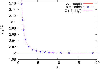
Figure 9: The numerical results for the magnetic susceptibility. On the left we show the result at $\theta=0$, which follows the formula (2.10) to an excellent accuracy. The plot on the right is our result for $\chi_{m}(\theta)/\xi(\theta)$. The data are reliable over the plotted range, before getting too close to $\pi$. This result was accessible with the multi-cluster algorithm along with an improved estimator.

At non-zero $\theta$, the result emerges from re-weighting the data of $\theta=0$ according to the prescription in Ref. [24]. The results are shown in Figure 9 on the right. We applied an improved estimator by flipping a number of clusters. Here we do consider the $\theta$-dependence of the correlation length, which is used to build the dimensionless ratio plotted in Figure 9. It grows rapidly as $\theta$ approaches $\pi$, cf. Figure 5, hence we involved quite long spin chains. Once $\xi(\theta)$ exceeds $L$, the considered ratio drops towards $0$, as we see from eq. (2.9). However, for a continuum limit $\theta\to\pi$ which respects $L\gg\xi$ the plateau at relatively large $\theta$ suggests a value $\chi_{m}(\theta)/\xi(\theta)\approx 1$.

In one case, $\beta=5$, $L=300$, we indicate jackknife errors. In the other cases they are similar, i.e. again very small up to the close vicinity of $\theta=\pi$. This is very remarkable in view of the generic difficulties to obtain numerical results for models with a significant imaginary part in the Euclidean action.

The statistics includes several millions of configurations, and it is still enhanced thanks to the improved estimator. In particular, statistics in a fixed topological sector can be cumulated by flipping neutral clusters. In this way it could be simulated within a few weeks on a 2 GHz machine; with the Metropolis algorithm this measurement is hardly feasible.

5 Conclusions and outlook

We presented a new and successful application of the meron cluster algorithm. In the spin chains that we considered, it provides precise simulation results in a highly efficient way. We assigned a half-integer topological charge to each cluster, which is the basis of a powerful improved estimator. This yields accurate result for the present toy model with a $\theta$-term — an issue, which is still outstanding in QCD.

Here it was possible to suppress the notorious problem of critical slowing down. With respect to the topological charge we overcome this problem completely. Regarding the energy, the dynamical critical exponent is reduced by almost a factor of $4$.

This provides a strong motivation to search for applications of this technique also in higher dimensions, i.e. in field theoretic models. In particular an application of the meron cluster algorithm in the 3d $O(4)$ model appears promising — that model can be interpreted as an effective description of QCD with two light quark flavours at high temperature.

We add a very rough estimate about the feasibility of that project. If $\xi(\theta)$ behaves similarly to Figure 5, we control the finite size effects quite well up to $\theta\approx 0.9\,\pi$ for instance with $L=32$. Compared to the spin chains that we considered to measure $\chi_{m}(\theta)/\xi(\theta)$, this implies a factor of $O(100)$ for the number of lattice sites (along with a factor of $6$ for the generators of the symmetry group). Tiny error bars as we obtained in Figure 9 (on the right) may be relaxed without problems, say by a factor $\mathop{\raise 1.29167pt\hbox{$>$\kern-7.5pt\raise-4.73611pt\hbox{$\sim$}}}3$, so that the required statistics decreases by an order of magnitude. Comparing now to the computational effort which was necessary in $d=1$ (cf. last paragraph in Section 4), and considering the option to use a number of processors simultaneously, we estimate that the 3d $O(4)$ model at finite $\theta$ can be solved to a good precision with the meron cluster algorithm within less than one year.

Acknowledgements: We thank Michael Müller-Preußker, André Sternbeck, Jan Volkholz, Uwe-Jens Wiese and Ulli Wolff for useful comments. The computations were performed on a PC cluster at the Humboldt-Universität zu Berlin.

References

- [1]
- [2] R.H. Swendsen and J.S. Wang, Phys. Rev. Lett. 58 (1987) 86.
- [3] U. Wolff, Phys. Rev. Lett. 62 (1989) 361.
- [4] F. Niedermayer, Lectures given at Eötvös Summer School “Advances in Computer Simulation”, Budapest 1996 [hep-lat/9704009].
-
[5]
R. Sinclair,
Phys. Rev. D45 (1992) 2098.
F. Alet, B. Lucini and M. Vettorazzo, Comput. Phys. Commun. 169 (2005) 370. - [6] K. Langfeld, M. Quandt, W. Lutz and H. Reinhardt, hep-lat/0606009.
- [7] Y. Tomita and Y. Okabe, Phys. Rev. B65 (2002) 184405.
- [8] M. del Pilar Monsiváis-Alonso,“Simulations in statistical physics and biology: some applications”, M.Sc. thesis, San Luis Potosí, México (2006) [physics/0603035].
- [9] Y. Deng, W. Guo and H.W.J. Blöte, cond-mat/0605165.
- [10] W. Bietenholz, A. Pochinsky and U.-J. Wiese, Phys. Rev. Lett. 75 (1995) 4524; Nucl. Phys. (Proc. Suppl.) B47 (1996) 727.
- [11] F. Brechtefeld, hep-lat/0207012.
-
[12]
S. Chandrasekharan and U-J. Wiese,
Phys. Rev. Lett. 83 (1999) 3116.
S. Chandrasekharan, J. Cox, K. Holland and U.-J. Wiese, Nucl. Phys. B576 (2000) 481.
S. Chandrasekharan and J.C. Osborn, Phys. Lett. B496 (2000) 122.
S. Chandrasekharan, J. Cox, J.C. Osborn and U.-J. Wiese, Nucl. Phys. B673 (2003) 405. - [13] T. Boyer, “Chaîne de spins dans le modèle XY: Investigation par un algorithme multi-clusters”, B.Sc. Thesis, Berlin and Paris (2005).
-
[14]
O. Philipsen,
PoSLAT(2005)016 [hep-lat/0510077].
M.A. Stephanov, PoSLAT(2006)024 [hep-lat/0701002].
D.K. Sinclair, hep-lat/0701010. - [15] W. Bietenholz, R. Brower, S. Chandrasekharan and U.-J. Wiese, Phys. Lett. B407 (1997) 283.
-
[16]
T.L. Bell and K.G. Wilson,
Phys. Rev. B11 (1975) 3431.
W. Bietenholz, Int. J. Mod. Phys. A15 (2000) 3341. - [17] B. Berg and M. Lüscher, Nucl. Phys. B190 (1981) 412.
- [18] M. Lüscher, Commun. Math. Phys. 85 (1982) 39.
- [19] R.G. Edwards and A.D. Sokal, Phys. Rev. D40 (1989) 1374.
- [20] U. Wolff, Phys. Lett. B222 (1989) 759.
- [21] B.B. Beard, M. Pepe, S. Riederer and U.-J. Wiese, Phys. Rev. Lett. 94 (2005) 010603.
-
[22]
J. Ambjørn, K.N. Anagnostopoulos,
J. Nishimura and J.J.M. Verbaarschot, JHEP 0210 (2002) 062.
V. Azcoiti, G. Di Carlo, A. Galante and V. Laliena, Phys. Lett. B563 (2003) 117.
M. Imachi, Y. Shinno and H. Yoneyama, Prog. Theor. Phys. 111 (2004) 387. - [23] E.-M. Ilgenfritz, M.L. Laursen, G. Schierholz, M. Müller-Preußker and H. Schiller, Nucl. Phys. B268 (1986) 693.
- [24] U.-J. Wiese, Nucl. Phys. B318 (1989) 153.