Prospects of Transition Interface Sampling simulations for the theoretical study of zeolite synthesis

Abstract

The transition interface sampling (TIS) technique allows to overcome large free energy barriers within reasonable simulation time, which is impossible for straightforward molecular dynamics. Still, the method does not impose an artificial driving force, but it surmounts the timescale problem by an importance sampling of true dynamical pathways. Recently, it was shown that the efficiency of TIS to calculate reaction rates is less sensitive to the choice of reaction coordinate than those of the standard free energy based techniques. This could be an important advantage in complex systems for which a good reaction coordinate is usually very difficult to find. We explain the principles of this method and discuss some of the promising applications related to zeolite formation.

I Introduction

Gaining insight in the zeolite formation has not only fundamental scientific importance, but could also accelerate momentous technological developments. The applications of zeolites are uncountable ranging from cracking catalysis of crude oil, gas separation, detergent builders, and sensors for pharmaceutical formulations. The specific catalytic properties of zeolites lie in their unique open crystalline structure that incorporates cages or channels with typically nanoscale diameters. The growth of the open structure silicon dioxide polymorphs is mediated by so-called template molecules that can be removed out of the zeolite pores after the crystallization process. Besides template molecules, solvent, Si/Al ratio, temperature, pH, and many other factors play a role in determining which zeolite topology is formed. As each structure and composition has its unique catalytic properties, the synthesis of new zeolite materials has been an important branch of chemical research. This development has progressed mainly on the basis of trial-and-error and ’chemical intuition’ as a fundamental understanding of zeolite formation is lacking. The clear solution synthesis studies of silicalite-1 zeolites initiated by Schoeman et al.schoeman94 were an important step forward for the experimental analysis. The use of clear solutions instead of gels made the analysis of zeolite synthesis much more accessible by experimental techniques. Since then, this model system has been subject of many studies including x-ray and neutron scattering, infrared (IR) spectroscopy, Nuclear magnetic resonance (NMR), and dynamic light scattering (DLS). These studies revealed that upon mixing tetraethylorthosilicate (TEOS), tetrapropylammonium hydroxide (TPAOH) and water at a certain ratio at room temperature sub-colloidal particles are formed of several nanometers. Using the freeze drying technique schoeman96 ; freeze2 , these particles have been extracted from the solution and examined by various techniques such as solid state NMR, Fourier Transform IR (FTIR), transmission electron microscopy (TEM), and atomic force microscopy (AFM). Various models for the structure of these particles have been proposed ranging from amorphous bodies kragten03 ; Rimer06 to precise framework fragments nanoslab1 .

The formation of crystalline zeolite particles is initiated when this suspension is heated upto temperatures of 350 K. Light scattering experiments show that the intensity scattered by the suspension increases only slowly in time during the first period of the synthesis. This is then followed by a sharp increase, indicating the starting point of growth of what will become the final crystals. The first period can be associated to a nucleation process, in which a particle has to be formed with a size beyond its critical nucleation radius. The formation of zeolites consist hence of several stages. First a polymerization process which eventually leads to the formation of sub-colloidal particles, second the nucleation process, and finally the crystal growth.

One of the difficulties in the investigation of the zeolite formation process is that the relevant lengthscales of the zeolite formation lie just in between the accessible lengthscale of NMR and diffraction techniques auerbach05 . Moreover, it is unclear if freezed-dried extractions are identical to the silicate particles existing in solution. Since many experiments do not allow unequivocal interpretation, it is not a surprise that several crystallization mechanisms have been proposed. These theories concentrate on the structure and shape of the colloidal particles, how these particles are formed and how these particles finally contribute in the formation of the zeolite crystal.

An example is the nanoslab hypothesis that was postulated by some of us. It was inspired by several experimental observations nanoslab1 ; nanoslab2 ; nanoslab3 . This theory assumes that at an initial stage precursor particles are formed that consist of 30 to 33 Si atoms enclosing a single template molecule. These precursors stick together in a block shaped particle, the nanoslab, that has already the correct crystalline structure. These particles finally form the zeolite by a ’clicking-mechanism’ when the solution is heated up. Others have claimed that the apparent evidence of the Si-30/33 precursor particle should be attributed to other Si containing species knight06 or that the nanoshaped particle is actually an amorphous identity with a layer of template molecules around it kragten03 ; Rimer06 . Also the role of the nanosized particles for the nucleation and crystal growth has been subject of debate. According to some groups, the nanoparticles add one by one to the growing crystals niko2000 ; dokter . Others regard the particles as monomer reservoirs: monomer dissolves into the solution and attaches to the growing nucleus Schoeman98 ; cundy . Recent publications davis ; cundy state that an aggregative growth mechanism of discrete nanoparticles may dominate the early stage of the growth process. However, after a certain size is attained, the growth mechanism seems to switch to addition of low molecular species, probably monomers.

In conclusion, despite many years of abundant experimental research, zeolite synthesis still contains many mysteries. Therefore, this field of research is a prototype example where computer simulations could give invaluable information. However, before truly realistic simulations of all stages in the zeolite synthesis can be performed, a long way has to be gone. Reason for the difficulty is that the typical system sizes and timescales at which the zeolite formation takes place are generally beyond the capabilities of present computer resources. For a correct modeling of the nucleation process, the simulation box should at least be larger than the critical nucleus. A requirement that is out of limits for quantum mechanical calculations and demands the development of accurate reactive forcefields.

So far fully quantum mechanical calculations using Density Functional Theory (DFT) have been applied to silica polymerization clusters Pereira1 ; Pereira2 . These studies showed a stronger stability of silicate 6 rings and linear polymers compared to smaller rings and branched polymers. Ph effects were considered in [Lewis2, ; Thuat, ] by analyzing negatively charged silica clusters that are favorable to neutral ones in an alkaline environment. This study revealed that internal cyclization if preferred over further linear growth Lewis2 . Barriers for oligomerization were significantly reduced for single charged cluster compared to neutral ones Thuat .

Based on ab initio calculations or experimental data, several classical forcefields have been developed catlow2 ; aoki ; vashista ; beest ; feuston . These potentials allow the study of larger systems including solvent and template molecules. However, the existing potentials are not yet very accurately describing the breaking and making of chemical bonds, which presumably requires complex many-body terms and polarizable forcefields. Still, studies using these approximate potentials can give valuable insights. For instance, classical molecular dynamics (MD) simulations have shed some light to the role of solvent and template molecules Catlow1 ; Lewis . These simulations showed that, contrary to fully formed cages and rings, open structures collapse in the presence of solvent, unless it contained strongly bonded template molecules. The early stages of silica polymerization dynamics were studied by Rao and Gelb Rao at high temperatures $\gtrsim 1500$ K. These alleviated temperatures were required as upto $600$ K, no polymerization reaction could be observed within the nanoseconds simulation periods. They found that both the monomer incorporation and the cluster-cluster aggregation were important mechanisms for diluted solutions, while the first mechanism was dominant in the concentrated systems. Using a implicit solvent model not including template molecules, Wu and Deem analyzed the free energy barriers and critical cluster sizes as function of pH and Si-monomer concentration at ambient conditions using a series of advanced Monte Carlo (MC) techniques Deem1 . They found that the critical clusters for the polymerization contained relatively few ($\approx 30-40$) Si atoms. No attempt was made to derive reaction rates by calculating transmission coefficients. Even larger systems and timescales have been simulated using lattice models auerbach05jacs ; Gubbins and kinetic MC (KMC) G78 . Relative rates for different crystal growth mechanisms via kink and edge sites can be derived by mimicking atomic force micrographs via atomistic simulations agger1 ; agger2 ; agger3 . Still, even KMC simulations are usually restricted to growth gale1 ; gale2 . The time, before the critical nucleus of a zeolite is formed, is still too long even for this ultrafast type of dynamical simulations.

It is clear that the simulation methods have made significant progress in recent years. At the early stages of Si polymerization, fully quantum mechanical MD studies are in our reach using Born-Oppenheimer marx or Car-Parrinello marx ; cp simulations. Thanks to newly developed potentials and coarse grained systems, simulations approach the system sizes that are needed to describe the template directed zeolite synthesis in solution. Nonetheless, each stage in the zeolite synthesis involves significant reaction barriers. This makes the chance to observe important reactive events at experimental conditions within the duration of the simulation period highly unlikely. The reaction itself is usually very fast and could fit perfectly within the window of timescales that are attainable by the simulation method. However, the system will likely spend extensively long periods within the well of the reactant state without any reactive event taking place. It is, therefore, important to have a method that focuses the costly simulation time on the important but rare reactive events, while limiting the superfluent exploration of the reactant well. In this article, we review such a method, the transition interface sampling (TIS) ErpMoBol2003 ; titusthesis ; ErpBol2004 method, that allows to concentrate only on those trajectories that are important for the chemical process. Moreover, the TIS technique can calculate the frequency for occurrence of these successful trajectories within an infinitely long straightforward simulation. Hence, TIS allows the determination of the rate of the rare event.

The aim of this article is not to give a fully detailed theoretical derivation of the method. This has already been published elsewhere ErpMoBol2003 ; titusthesis ; ErpBol2004 . The goal of this article is to give an educative overview of the practical algorithms and their possible applications related to zeolite studies rather than on mathematical aspects.

II Transition Interface Sampling

II.1 historic perspectives of rare event simulations

The first theories for treating rare events from a microscopic perspective where pioneered by Eyring E35 , Wigner W38 , and Horiutu H38 about 20 years before the first MD simulation was performed Alder . They introduced the concept of Transition State (TS) and the so-called TS Theory (TST) approximation. Later Keck demonstrated how the TST approximation can be made exact by a dynamical correction, the transmission coefficient Keck67 . The actual application of these theories for molecular simulation was directed by the works of Bennett Bennet77 and Chandler DC78 , which have made this a standard approach in molecular simulation. A crucial point in this reactive flux (RF) method is the definition of a suitable reaction coordinate (RC). As a first step, the free energy needs to be determined along this RC using importance sampling techniques such as Umbrella Sampling (US) TV74 or Thermodynamic Integration (TI) CCH89 . This result alone is sufficient to obtain the TST approximation of the rate, which is an upper limit for the actual rate. In the second step, the correction to this approximation can be calculated by releasing dynamical trajectories from the top of the free energy barrier. Only when both steps are completed, the exact reaction rate can be calculated. Both the free energy barrier and the transmission coefficient depend on which RC is taken, but the final result that combines the two outcomes is independent of this choice.

The RF method as proved its value for many systems, but also has its drawbacks. Although its result is independent of the chosen RC, its efficiency does and sensitively determines its success or failure. A non-suitable choice of RC can result in hysteresis effects in the free energy calculation, which frustrates an accurate estimation of the barrier. Besides, even if an accurate value for the free energy barrier can be obtained, the corresponding transmission coefficient will be very small and its evaluation will require an extremely large number of pathways. In practice, it has been experienced that finding a good RC can be extremely difficult in high dimensional complex systems. Notable examples are chemical reactions in solution, where the reaction mechanism often depends on highly non-trivial solvent rearrangements. Also, computer simulations of nucleation processes use very complicated order parameters to distinguish between particles belonging to the liquid and solid phase. This makes it unfeasible to construct a single RC that accurately describes the exact place of cross-over transitions. As result, hysteresis effects and low transmission coefficients are almost unavoidable.

The problem of finding suitable RCs, has urged the development of alternative methods. In 1998, Dellago et al. came up with such an alternative method that they called transition path sampling (TPS) TPS98 ; TPS98_2 ; TPS98_3 ; TPS99 . This approach can be described as a MC sampling of MD pathways. Using a detailed balance technique, a set of trajectories can be collected that satisfy some predetermined criteria. For instance, one can constrain the start- and end-point of the path in such a way that each trajectory connects the reactant and product state. An important point is that this sampling of successful reactive events does not require a RC that captures the reactive mechanism, but only needs an order parameter that can distinguish between reactant and product state. In addition to this, the first series of TPS papers TPS98 ; TPS98_2 ; TPS98_3 ; TPS99 also provided a route to calculate reaction rates. However, this approach has seldom been used due to its high computational cost. Moreover, within the context of the reaction rate calculation, it is not so obvious to state that the TPS order parameter is actually very different from a RC. In this approach, the end-point of the path is forced to progress in successive steps from reactant to product state. Hence, the TPS order parameter needs to describe the intermediate states as well just as a RC in the standard methods.

Luckily, the algorithmic procedure to calculate reaction rates using the same path sampling framework improved considerably when the transition interface sampling (TIS) technique was devised ErpMoBol2003 . TIS uses a flexible pathlength which reduces the number of required MD steps significantly. Moreover, the TIS method also eliminates the need of so-called MC shifting moves that required a considerable percentage of the simulation time in the TPS scheme. In addition, one can show that the new mathematical formulation of the reaction rate is less sensitive to recrossing events which guarantees a faster convergence.

While TPS imposes conditions to the start- and end-point of the path to be within certain intervals of the RC, TIS imposes an interface crossing condition. Except for the technique proposed in Ref. [ErpBol2004, ], TIS needs a RC just like the original TPS scheme. The RC is required to define a set of interfaces between the stable reactant and product states. However, unlike the standard RF methods, the TIS efficiency is relatively insensitive to the choice of RC as was first proven in [TISeff, ]. This point is a strong advantage in complex systems where a ’good RC’ can be extremely difficult to find.

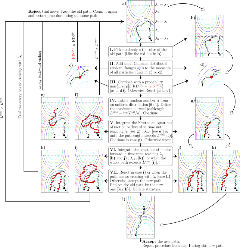
Figure 1: Illustration of the shooting algorithm in TIS. The panels a)-l) depict trajectories/trajectory-segments on a free energy surface. The dashed horizontal lines are the TIS interfaces ($n=4$ and $i=2$ in this case). The algorithm requires an initial path a) to start the loop. The length of this particular path $L^{(o)}$ is eighteen timeslices (endpoints are not included). At step I, a random point is picked from this old path and some small randomized changes are applied to the velocities of all the particles (II), followed by a Metropolis acceptance/rejection step (III). In c) the new velocities have resulted in a much larger kinetic energy ${\rm KIN}^{(n)}$ and therefore this trial move is most likely rejected. Step IV is requir ed to maintain detailed balance between pathways of different lengths. For example, if the random number generator assigns $\alpha=.59$ then $L^{\rm max}=30$ and we can reject when the path is unfinished, but already contains 31 timeslices as in panel f) and i). At V, the equations of motion are integrated backwards in time by a MD algorithm using the shooting point with reverse velocities as starting point. At VI) the equations of motion are integrated forward in time starting from the same shooting point (without reversed velocities). After a rejection the old path is kept and counted again. If accepted, the new path will automatically start at $\lambda_{A}$ and cross $\lambda_{i}$. The path can end at either $\lambda_{A}$ as in j) or at $\lambda_{i+1}$ as in k). The fraction of sampled pathways that end at $\lambda_{i+1}$ determines ${\mathcal{P}}_{A}(\lambda_{i+1}|\lambda_{i})$

II.2 the TIS algorithm

The TIS algorithm works as follows. First step is to define a RC and a set of related values $\lambda_{0},\lambda_{1},\ldots,\lambda_{n}$ with $\lambda_{i}<\lambda_{i+1}$. The subsets of phase- or configuration points for which the RC is exactly equal to $\lambda_{i}$ basically define multidimensional surfaces or interfaces which give the name to this method. These values/interfaces should obey the following requirements: if the RC is lower than $\lambda_{0}=\lambda_{A}$, the system should be in the reactant state $A$; if the RC is higher than $\lambda_{n}=\lambda_{B}$ the system should be in the product state $B$; $n$ and the positions for the interfaces in between, $\lambda_{i}$ with $1=1,2,\ldots,n-1$, should be set to optimize the efficiency. Further, the surface $\lambda_{A}$ should be set in such a way that whenever a MD simulation is released from within the reactant well, this surface should be frequently crossed. The TIS rate expression can then be formulated as

$$k_{AB}=f_{A}\,{\mathcal{P}}_{A}(\lambda_{B}|\lambda_{A})$$ (1)

Here, $f_{A}$ is the escape flux through the first interface. In a long MD simulation, this simply corresponds to the number of detected crossings through the surface $\lambda_{A}$ divided by the total simulation time (here, we assume that we will not observe a spontaneous transition to state $B$ during the simulation. For a more formal definition see [ErpMoBol2003, ]). The other term ${\mathcal{P}}_{A}(\lambda_{B}|\lambda_{A})$ is the overall crossing probability. This is the probability that whenever the system crosses $\lambda_{A}$, it will cross $\lambda_{B}$ before it crosses $\lambda_{A}$ again. As $\lambda_{B}$ is a surface at the other side of the barrier, this probability will be very small and can not be calculated directly. This probability can, however, be determined by a series of path sampling simulations using the following factorization:

$${\mathcal{P}}_{A}(\lambda_{B}|\lambda_{A})={\mathcal{P}}_{A}(\lambda_{n}|\lambda_{0})=\prod_{i=0}^{n-1}{\mathcal{P}}_{A}(\lambda_{i+1}|\lambda_{i}).$$ (2)

The terms ${\mathcal{P}}_{A}(\lambda_{i+1}|\lambda_{i})$ are history dependent conditional crossing probabilities which are much higher and can be computed. In words, ${\mathcal{P}}_{A}(\lambda_{i+1}|\lambda_{i})$ is the probability that $\lambda_{i+1}$ will be crossed before $\lambda_{A}$ under the twofold condition that the system is at the point to cross the interface $\lambda_{i}$ in one timestep while $\lambda_{A}$ was more recently crossed than $\lambda_{i}$ in the past. It is due to this history dependence that Eq. (2) is exact and should not be misinterpreted as a Markovian approximation. ${\mathcal{P}}_{A}(\lambda_{i+1}|\lambda_{i})$ is also equal to the number of all possible paths that start at $\lambda_{A}$ and end at $\lambda_{i+1}$ divided by the number of all possible paths that start at $\lambda_{A}$, end at either $\lambda_{i+1}$ or $\lambda_{A}$, and have at least one crossing with $\lambda_{i}$. Hence, this term can be calculated if we can generate the appropriate trajectories with their correct statistical weight. It is however not so obvious to generate these pathways especially when $\lambda_{i}$ is in the reaction barrier region. This difficulty can be overcome by a MC algorithm that employs a variation of the TPS shooting move. The algorithm is explained in Fig. 1.

The algorithm requires to have one path fulfilling the correct condition. That is starting at $\lambda_{A}$ and crossing $\lambda_{i}$ at least once before ending at either $\lambda_{i+1}$ or $\lambda_{A}$. A crucial point is step II. After picking a random timeslice (a point that constitutes all the particle positions and momenta at a certain timestep along the path), one adds random values to all the momenta. In practice, these random values are taken from a Gaussian distribution with a certain width $\sigma$, that should be adapted to obtain the optimum efficiency. If $\sigma$ is small, the random momentum changes will be small as well and the new path will lie closely to the old one (if we assume deterministic dynamics). This small deviation results in a significant chance that the trial path will satisfy the required conditions as well which yields a good acceptance rate. However, a too small value of $\sigma$ will result in too strong correlations between the accepted moves (In the extreme case when $\sigma=0$, one regenerates exclusively the same path). Usually, one tries several values for $\sigma$ in a series of short test simulations. It is generally assumed that the value that yields an acceptance rate of 50 % is close to an optimum value for $\sigma$. If one wants to simulate at constant energy instead of constant temperature, step III can be replaced by a proper velocity rescaling procedure that, if needed, can also preserve linear and angular momentum GDC99_2 .

Another important point is that, in order to enter the loop, one needs to have a single path that obeys the correct requirements. This can already be quite difficult and several techniques to get such a first initial path have been suggested BolAnnu . However, in TIS these initial paths are generated automatically when the different types of simulations are consecutively performed (See Fig. 2).

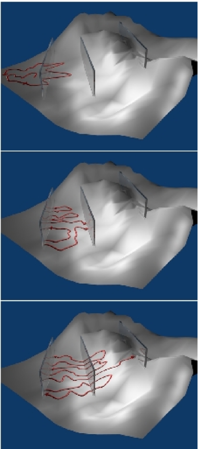
Figure 2: This pictures illustrates some typical trajectories on a free energy surface for a series of TIS simulations. The glassy plates represent the TIS interfaces. The first type of simulation (top), is a straightforward MD simulation which is required to calculate the flux $f_{A}$ through the first interface. The next step is a path-sampling simulation which generates pathways that start at $\lambda_{A}$ and end at either $\lambda_{A}$ or $\lambda_{1}$. This simulation yields the result of ${\mathcal{P}}_{A}(\lambda_{1}|\lambda_{0})$ and is illustrated in the middle panel. The initial path to start this simulation can be obtained by taking a trajectory segment from the initial MD simulation. The bottom panel shows the next path-sampling simulation to calculate ${\mathcal{P}}_{A}(\lambda_{2}|\lambda_{1})$. It generates pathways that start at $\lambda_{A}$ and cross $\lambda_{1}$ at least once. Also here, the initial path can be obtained from the previous simulation by taking one of the paths that successfully reached $\lambda_{1}$.

First the MD simulation is performed to calculate $f_{A}$. Then, a series of path-sampling simulations follows to calculate ${\mathcal{P}}_{A}(\lambda_{1}|\lambda_{0}),{\mathcal{P}}_{A}(\lambda_{2}|\lambda_{1}),\ldots,{\mathcal{P}}_{A}(\lambda_{n}|\lambda_{n-1})$. When these simulations are performed in this order, each path-sampling simulation can obtain the necessary initial path from the previous simulation (See Fig. 2).

It is important to note that the final result, the reaction rate $k_{AB}$, does not sensitively depend on the positions of the outer interfaces $\lambda_{A}$ and $\lambda_{B}$ as long as they are reasonable. The number of interfaces $n$ and their positions only influence the efficiency of the method. It was found that the total efficiency is optimized when for each path-simulation one out of five trajectories reaches the next interface ErpBol2004 ; TISeff . Hence, using some initial trial simulations, one can adjust the number of interfaces and their position to satisfy this condition. The easiest way to achieve this is to use a slight variation of the algorithm that is shown in Fig. 1. Instead of stopping the integration when the trajectory crosses $\lambda_{i+1}$ as in panel e) and k), one can continue the trajectory until it reaches $\lambda_{A}$ or $\lambda_{B}$. This algorithm only requires knowing the position of $\lambda_{A}$, $\lambda_{B}$, and $\lambda_{i}$. By examining the progress of the paths along the RC beyond $\lambda_{i}$, one can define the next interface $\lambda_{i+1}$ exactly at the point where 80 % of the paths have returned to $\lambda_{A}$.

II.3 analysis of the reaction mechanism

When the complete series of simulations is finished, the reaction rate follows simply from Eqs. (1,2). In addition to this, the ensemble of pathways can be analyzed which can yield valuable information about the reaction mechanism. In this respect, the TIS path-ensembles might actually prove to be more useful than the ones obtained by the original TPS method. As each ensemble contains the correct ratio of paths progressing upto a certain level, but then either return or make a little step further, one can try to understand the characteristic differences between the ’successful’ and unsuccessful’ pathways. In contrast, the TPS method aims to generate successful trajectories only. One of the properties that can improve understanding of mechanisms is the overall crossing probability function. This represents a sort of path survival probability along the RC. This function equals 1 at $\lambda_{0}$ and $P_{A}(\lambda_{B}|\lambda_{A})$ at $\lambda_{B}$. In transition, this function is monotonically decreasing and terminates in a horizontal plateau when the barrier ridge is crossed completely. This function could be considered as a dynamical equivalent of the free energy profile along the RC. In Fig. 3 the overall crossing probability function is depicted together with the free energy profile obtained from a nucleation process of Lennard-Jones particles.

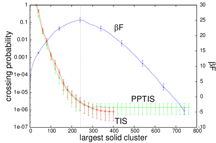
Figure 3: The crossing probability function obtained by TIS and partial path TIS (PPTIS) MoBolErp2004 for nucleation process of LJ particles. The simulation data are obtained from [MoBolPRL, ]. The free energy profile, that was calculated simultaneously using the technique of [MoErpBol, ], is also shown. The simulated system contained 10648 particles in total. The RC was defined as the largest solid cluster in the system. More details can be found in  [MoBolPRL, ]. The final crossing probability was $P_{A}(\lambda_{B}|\lambda_{A})=(7.8\pm 5.5)\cdot 10^{-7}$ (TIS) and $(14.1\pm 8.7)\cdot 10^{-7}$ (PPTIS). The crossing probability shows a plateau at 410.5 indicating that the reaction barrier ridge is crossed. The free energy barrier has a maximum at 243. After this point about 50 % (PPTIS) till 75 % (TIS) of the paths still fail to reach the reactant state. Although, the PPTIS and TIS results are within each others error-bars, it is likely that PPTIS overestimates the crossing probability due to the imprecise choice of RC TISeff .

The results were obtained from from Ref. [MoBolPRL, ]. Interestingly, after the maximum of free energy barrier is crossed (cluster size 243), the majority of the trajectories ($\sim 75\%$) still fail to reach the reactant state. This effect might be partly due to diffusive motion, but is most likely an effect of an improperly chosen RC. This shows that the projection on a single RC using static free energy calculations can be misleading. Neither the height of the barrier nor the position of the TS dividing surface have to reflect the actual height and position of the reaction barrier. Indeed, Moroni et al. found that a ’good RC’ should at least incorporate one more important quantity which is the crystallinity of the cluster. Small clusters $<243$ with a high crystallinity were found to grow further easily, while large clusters with less structure were unstable and broke-up into smaller pieces.

II.4 recent and future developments and applications

Besides an efficient algorithm for the calculation of reaction rates, the TIS method has provided a new mathematical framework to describe rare events. Recent new simulation techniques have exploited this TIS theory. For example, for diffusive barrier crossings, where transition paths become very long, the partial path TIS (PPTIS) method was devised MoBolErp2004 . Here, using the assumption of memory loss, much shorter paths are generated after which the overall crossing probability can be reconstructed by a recursive formulation. The forward flux sampling technique FFS ; FFS2 is basically the same as TIS, but the way to generate pathways is different. In this approach, the endpoints of all the pathways successfully reaching the next interface are stored and starting from each point a set of new pathways is generated in the next simulation. The main advantage is that the FFS scheme supplies a route to handle non-equilibrium systems. A disadvantage is that this only works for stochastic dynamics and will always yield much stronger correlations between the generated pathways and the different path ensembles even for the pure Brownian dynamics case. Another drawback of PPTIS and FFS methods is that they do not possess the same RC insensitivity as TIS TISeff . If necessary, even a fully RC free approach is possible as was suggested in [ErpBol2004, ] using the TIS pathlength as a transition parameter. A nice feature of this approach is that it does not require to specify a specific product state. Combinations with Configurational Bias MC ErpBol2004 ; FFS2 and path swapping techniques ErpBol2004 ; ErpInPr may also yield promising advances for the computational efficiency.

The TIS and its variations have been applied to various systems ranging from simple test-systems ErpMoBol2003 ; MoBolErp2004 , nucleation MoBolPRL ; Valer ; Sear , protein folding bolhuisPNAS ; pfold2 , biochemical networks FFS , driven polymer translocation through pores FFS2 , micelle formation thesisRene , ab initio simulation of chemical reactions titusthesis and DNA denaturation ErpInPr .

The TIS technique can open many possible avenues in the field of zeolite formation simulations at several stages of the process. For instance, the first elementary step to Si polymerization is the condensation reaction 2Si(OH)${}_{4}\rightarrow$ Si₂O(OH)₆+H₂O. This has been studied by ab initio static analysis including implicit solvent Pereira3 . This study has revealed two possible reaction mechanisms. Such a system is small enough to be treated by ab initio MD marx ; cp including explicit solvent molecules. The TIS method could hence give valuable insight which reaction mechanism dominates when dynamics and explicit solvent is taken into account. Classical reactive forcefields and rare event methods, such as TIS and PPTIS, should make it possible to simulate the dynamics of Si polymerization at much lower temperatures than hitherto was possible RaoGelb . This allows to study this process at conditions that are much closer to the experimental situation. Moreover, by a right construction of the interfaces, the TIS method allows to focus on reaction mechanisms and rates of some very specific polymerization reactions, for instance the formation of the Si-30/33 precursor nanoslab2 .

With the development of lattice and KMC models, the study of the next stages of nucleation and zeolite growth also come into reach. The combination of KMC and path sampling is a promising yet unexplored territory. Despite the enormous long simulation periods that can be achieved by KMC, the expectation time to form a critical nucleus starting from a disorder solution is generally still out of reach. Therefore, most KMC studies have concentrated on growth rather than nucleation. Hence, the study of zeolite nucleation might benefit significantly using combined KMC and path sampling techniques.

III Summary

We have reviewed the TIS method, its variations and its possible applications for the theoretical study of zeolite synthesis. The TIS method is a an elegant approach circumventing the timescale problem not by speeding up the dynamics of the system itself, but by concentrating on the short time trajectories which are of interest without using any approximation. TIS allows to overcome reaction barriers by a sequence of simulation series. It is important to realize that the barrier crossing event is not enhanced due to some artifical force but only due to the MC acception/rejection steps that include the interface crossing condition. Hence, each trajectory in the TIS path ensembles satisfy the correct dynamics on the true potential energy surface. This makes the method fundamentally different from, for instance, the metadynamics LP02 approach. The TIS method makes use of the fact that the time needed to actually cross the barrier, the transition time, is much shorter than relaxation time $k_{AB}^{-1}$, which is the time wherein one can expect a reactive event from an arbitrary point within the reactant well.

TIS can be combined with any type of dynamics such as ab initio MD, Langevin, pure Brownian motion, classical MD and KMC. A requirement for application of this method is that the simulation of short trajectories can occur sufficiently fast. This limits the size of the systems which can be studied, ranging from several molecules for ab initio dynamics to several thousand molecules for MD, and even larger assemblies for KMC simulations.

Still, substantial work has to be done before fully realistic modeling of zeolite synthesis is our reach. An important requirement is the development of more accurate reactive force fields that can describe chemical events within the environment of solvent and template molecules. Recently, a more systematic approach for this development was suggested Toon . Even though, the lattice and KMC models are making substantial steps forward, inclusion of solvent effects in a lattice-type models has proven to be a difficult problem that has not yet been solved. To conclude, the simulation methods have made prodigious advancements in recent years and might ultimately give answers to important questions regarding zeolite synthesis, that can not be unambiguously accessed by experimental techniques. The TIS methods can help in obtaining dynamical information for the crucial but rare reaction steps in the zeolite process. In the near future, we are going to explore the application of TIS for the study of zeolite genesis.

- (1) B. J. Schoeman, , J. Sterte, and J. E., Zeolites, 1994, 14, 110–116.
- (2) J. Hedlund, B. J. Schoeman, and J. Sterte In ed. H. Chon, S.-K. Ihm, and Y. S. Uh, Progress in zeolites and microporous materials, pp. 2203–2210, Amsterdam, 1996. Elsevier.
- (3) R. Ravishankar, C. E. A. Kirschhock, B. J. Schoeman, P. Vanoppen, P. J. Grobet, S. Storck, W. F. Maier, J. A. Martens, F. C. D. Schrijver, and P. A. Jacobs, J. Phys. Chem. B, 1998, 102, 2633–2639.
- (4) D. D. Kragten, J. M. Fedeyko, K. R. Sawant, J. D. Rimer, D. G. Vlachos, R. F. Lobo, and M. Tsapatsis, J. Phys. Chem. B, 2003, 107, 10006.
- (5) J. D. Rimer, J. M. Fedeyko, D. G. Vlachos, and R. L. Lobo, Chem. Eur. J., 2006, 12, 2926–2934.
- (6) R. Ravishankar, C. E. A. Kirschhock, P. P. Knops-Gerrits, E. J. P. Feijen, P. J. Grobet, P. Vanoppen, F. C. D. Schrijver, G. Miehe, H. Fuess, B. J. Schoeman, P. A. Jacobs, and J. A. Martens, J. Phys. Chem. B, 1999, 103, 4960–4964.
- (7) S. M. Auerbach, M. H. Ford, and P. A. Monson, Curr. Opin. Colloid Interface Sci, 2005, 10, 220–225.
- (8) C. E. A. Kirschhock, R. Ravishankar, F. Verspeurt, P. J. Grobet, P. A. Jacobs, and J. A. Martens, J. Phys. Chem. B, 1999, 103, 4965–4971.
- (9) C. E. A. Kirschhock, R. Ravishankar, L. van Looveren, P. A. Jacobs, and J. A. Martens, J. Phys. Chem. B, 1999, 103, 4972–4978.
- (10) C. T. G. Knight, J. Wang, and S. D. Kinrade, Phys. Chem. Chem. Phys., 2006, 8, 3099–3103.
- (11) V. Nikolakis, E. Kokkoli, M. Tirrell, M. Tsapatsis, and D. Vlachos, Chem. Mater., 2000, 12, 845–853.
- (12) W. H. Dokter, H. F. Vangarderen, T. P. M. Beelen, R. A. van Santen, and W. Bras, Angew. Chem., 1995, 34, 73–75.
- (13) B. Schoeman, Micropor. Mesopor. Mater., 1998, 22, 9–22.
- (14) C. S. Cundy and P. A. Cox, Micropor. Mesopor., 2005, 82, 1.
- (15) T. M. Davis, T. O. Drews, H. Ramanan, C. He, J. S. Dong, H. Schnablegger, M. A. Katsoulakis, E. Kokkoli, A. V. McCormick, R. L. Penn, and M. Tsapatsis, Nature Mater., 2006, 5, 400–408.
- (16) J. C. G. Pereira, C. R. A. Catlow, and G. D. Price, J. Phys. Chem. A, 1999, 103, 3252–3267.
- (17) J. C. G. Pereira, C. R. A. Catlow, and G. D. Price, J. Phys. Chem. A, 1999, 103, 3268–3284.
- (18) M. J. Mora-Fonz, C. R. A. Catlow, and D. W. Lewis, Angew. Chem., 2005, 44, 3082–3086.
- (19) T. T. Trinh, A. P. J. Jansen, and R. A. van Santen, J. Phys. Chem. B, 2007, 110, 23099–23106.
- (20) C. R. A. Catlow, C. M. Freeman, M. S. Islam, R. A. Jackson, M. Leslie, and S. M. Tomlinson, Philos. Mag. A, 1988, 58, 123–141.
- (21) S. Tsuneyuki, M. Tsukada, H. Aoki, and Y. Matsui, Phys. Rev. Lett., 1988, 61, 869.
- (22) P. Vashista, R. Kalia, and J. Rino, Phys. Rev. B, 1990, 41, 12197.
- (23) B. W. H. van Beest, G. J. Kramer, and R. A. van Santen, Phys. Rev. Lett., 1990, 64, 1955.
- (24) B. P. Feuston and S. H. Garofalini, J. Phys. Chem., 1990, 94, 5351–5356.
- (25) C. R. A. Catlow, D. S. Coombes, D. W. Lewis, J. Pereira, and G. Carlos, Chem. Mater, 1998, 10, 3249–3269.
- (26) D. W. Lewis, C. R. A. Catlow, and J. M. Thomson, Faraday Discuss, 1997, 106, 451–471.
- (27) N. Z. Rao and L. D. Gelb, J. Phys. Chem. B, 2004, 108, 12418–12428.
- (28) M. G. Wu and M. W. Deem, J. Chem. Phys., 2002, 116, 2125.
- (29) M. Jorge, S. M. Auerbach, and P. A. Monson, J. Am. Chem. Soc., 2005, 127, 2005.
- (30) F. R. Siperstein and K. E. Gubbins, Stud. Surf. Sci. Catal., 2002, 144, 647–654.
- (31) D. T. Gillespie, J. Comput. Phys., 1978, 28, 395.
- (32) M. W. Anderson, J. R. Agger, N. Hanif, O. Terasaki, and T. Ohsuna, Sol. State. Sci., 2001, 3, 809–819.
- (33) M. W. Anderson, J. R. Agger, N. Hanif, and O. Terasaki, Microporous Mesoporous Mater., 2001, 48, 1–9.
- (34) J. R. Agger, N. Hanif, and M. W. Anderson, Angew. Chem., 2001, 40, 4065–4067.
- (35) S. Piana and J. D. Gale, J. Am. Chem. Soc., 2005, 127, 1975–1982.
- (36) S. Piana, M. Reyhani, and J. D. Gale, Nature, 2005, 438, 70–73.
- (37) D. Marx and J. Hutter In ed. J. Grotendorst, Modern Methods and Algorithms of Quantum Chemistry, pp. 301–449, FZ Jülich, 2000. NIC.
- (38) R. Carr and M. parrinello, Phys. Rev. Lett., 1985, 55, 2471–2474.
- (39) T. S. van Erp, D. Moroni, and P. G. Bolhuis, J. Chem. Phys., 2003, 118, 7762–7774.
- (40) T. S. van Erp Solvent effects on chemistry with alcohols PhD thesis, Universiteit van Amsterdam, 2003.
- (41) T. S. van Erp and P. G. Bolhuis, J. Comput. Phys., 2005, 205, 157–181.
- (42) H. Eyring, J. Chem. Phys., 1935, 3, 107.
- (43) E. Wigner, Trans. Faraday Soc., 1938, 34, 29.
- (44) J. Horiuti, Bull. Chem. Soc. Jpn, 1938, 13, 210.
- (45) B. J. Alder and T. E. Wainwright, J. Chem. Phys., 1957, 27, 1208.
- (46) J. C. Keck, Adv. Chem. Phys., 1967, 13, 85.
- (47) C. H. Bennett In ed. R. Christofferson, Algorithms for Chemical Computations, ACS Symposium Series No. 46, Washington, D.C., 1977. American Chemical Society.
- (48) D. Chandler, J. Chem. Phys., 1978, 68, 2959.
- (49) G. M. Torrie and J. P. Valleau, Chem. Phys. Lett., 1974, 28, 578.
- (50) E. A. Carter, G. Ciccotti, J. T. Hynes, and R. Kapral, Chem. Phys. Lett., 1989, 156, 472.
- (51) C. Dellago, P. G. Bolhuis, F. S. Csajka, and D. Chandler, J. Chem. Phys., 1998, 108, 1964.
- (52) C. Dellago, P. G. Bolhuis, and D. Chandler, J. Chem. Phys., 1998, 108, 9236.
- (53) P. G. Bolhuis, C. Dellago, and D. Chandler, Faraday Discuss., 1998, 110, 421.
- (54) C. Dellago, P. G. Bolhuis, and D. Chandler, J. Chem. Phys., 1999, 110, 6617.
- (55) T. S. van Erp, J. Chem. Phys., 2006, 125, 174106.
- (56) P. L. Geissler, C. Dellago, and D. Chandler, Phys. Chem. Chem. Phys., 1999, 1, 1317.
- (57) P. G. Bolhuis, D. Chandler, C. Dellago, and P. L. Geissler, Ann. Rev. Phys. Chem., 2002, 53, 291–318.
- (58) D. Moroni, P. R. ten Wolde PR, and P. G. Bolhuis, Phys. Rev. Lett., 2005, 94, 235703.
- (59) D. Moroni, P. G. Bolhuis, and T. S. van Erp, J. Chem. Phys., 2004, 120, 4055–4065.
- (60) R. J. Allen, P. B. Warren, and P. R. ten Wolde, Phys. Rev. Lett., 2005, 94, 018104.
- (61) R. J. Allen, D. Frenkel, and P. R. ten Wolde, J. Chem. Phys., 2006, 124, 024102.
- (62) T. S. van Erp, In Progress.
- (63) C. Valeriani, E. Sanz, and D. Frenkel, J. Chem. Phys., 2005, 122, 194501.
- (64) A. J. Page and R. P. Sear, Phys. Rev. Lett., 2006, 97, 065701.
- (65) P. G. Bolhuis, Proc. Nat. Acad. Sci. USA, 2003, 100, 12129–12134.
- (66) P. G. Bolhuis, Biophys. J., 2005, 88, 50–61.
- (67) R. Pool Coarse grained soap A molecular simulation study on Micelle formation in dilute surfactant solutions PhD thesis, Universiteit van Amsterdam, 2006.
- (68) J. C. G. Pereira, C. R. A. Catlow, and G. D. Price, Chem. Commun., 1999, 13, 1387–1388.
- (69) N. Z. Rao and L. D. Gelb, J. Phys. Chem. B, 2004, 108, 12418–12428.
- (70) A. Laio and M. Parrinello, Proc. Natl. Acad. Sci. USA, 2002, 99, 12562.
- (71) t. verstraelen, d. van neck, p. w. ayers, v. van speybroeck, and m. waroquier, submitted.
- (72) D. Moroni, T. S. van Erp, and P. G. Bolhuis, Phys. Rev. E, 2005, 71, 056709.