Noise spectrum of a tunnel junction coupled to a nanomechanical oscillator

Abstract

A nanomechanical resonator coupled to a tunnel junction is studied. The oscillator modulates the transmission of the junction, changing the current and the noise spectrum. The influence of the oscillator on the noise spectrum of the junction is investigated, and the noise spectrum is obtained for arbitrary frequencies, temperatures and bias voltages. We find that the noise spectrum consists of a noise floor and a peaked structure with peaks at zero frequency, the oscillator frequency and twice the oscillator frequency. The influence of the oscillator vanishes if the bias voltage of the junction is lower than the oscillator frequency. We demonstrate that the peak at the oscillator frequency can be used to determine the oscillator occupation number, showing that the current noise in the junction functions as a thermometer for the oscillator.

I Introduction

The recent years have seen the shrinking of mechanical components to micrometer and further to nanometer size, spawning the new field of nanomechanics. SchwRou05 ; Ble04 Manufacturing techniques borrowed from semiconductor chip manufacturing (see e.g. Ref. EkiRou05, ) as well as bottom up approaches utilizing nanotubes Saz04 make it possible to produce nanomechanical resonators with resonance frequencies presently demonstrated up to 1 GHz. Nanomechanical resonators are of interest for several reasons. In proposed tests of the limits of quantum mechanics one would like to investigate the decoherence behavior of superpositions of macroscopically distinct states, of e.g. a nanomechanical resonator.Leg02 ; MarSimPen03 Typical nanomechanical resonators contain a macroscopic number of atoms, $\sim 10^{7}$, making the amplitude of the basic mode a macroscopic observable. The signature of such superpositions is strongest for low oscillator occupation numbers. Presently obtainable resonator frequencies are high enough to make cooling to the ground state feasible. Experimental efforts are under way to reach the first goal necessary for these measurements, cooling a nanomechanical resonator to the ground state. NaiBuuLah06 ; LahBuuCam04 ; GigBohZei06 ; ArcCohBri06 ; KleBou06

Other applications include the use of nanomechanical resonators as ultra-sensitive force detectors. Mass detection with zeptogram resolution utilizing nanomechanical resonators has been realized only recently.YanCalFen06 Nanosized cantilevers can also be used to detect magnetic forces. Detection of a single electron spin using a nanomechanical cantilever has already been demonstrated. RugBudMam04 Nanomechanical resonators can also find an application in the context of quantum computing. Coherent mechanical oscillators are suggested as coupling elements between phase qubits in a solid state quantum computer. GelCle05 All the mentioned applications not only require the fabrication of a suitable oscillator but also a way to detect the motion of a nanomechanical resonator. Different schemes for detection have been proposed (see e.g. Ref. SchwRou05, ). The most promising candidates for sensitive readout are electrical devices, such as tunnel junctions or single electron transistors, incorporated on the same chip as the nanomechanical resonator.SchwRou05

In the light of the possible applications it is necessary to obtain a theoretical understanding of nanomechanical resonators interacting with electrical devices on a chip. Theoretical descriptions of charge dynamics influenced by an oscillator have, up to now, mainly used a master equation technique. Mozyrsky and Martin investigated the model, where the transmission coefficient of a tunnel junction depends on the position of a nearby harmonic oscillator, in the zero temperature limit. They found that the oscillator acquires an effective temperature proportional to the junction bias voltage and also find the influence of the oscillator on the junction current at zero temperature.MozMar02 Clerk and Girvin calculated the noise induced by a harmonic oscillator in a tunnel junction for dc and ac bias at zero temperature using a Markovian master equation.CleGir04 The authors, together with Khomitsky found the current in a tunnel junction influenced by an oscillator for arbitrary system parameters.WabKhoRam05 The current and the noise power spectrum for an asymmetric junction in the high voltage limit were also calculated. Smirnov, Mourokh and HoringSmiMouHor03 analyzed the position fluctuations in the stationary state of a nanomechanical oscillator coupled to a tunnel junction for an exponential dependence of the tunneling amplitude on the oscillator position as well as the current through the tunnel junction. The theoretical descriptions of a nanomechanical oscillator interacting with a single electron transistor concentrated on the effects the single electron transistor, acting as a non-equilibrium environment, has on the oscillator. Rodrigues and ArmourRodArm05 derived a master equation for an oscillator-single electron transistor system and investigated stationary state properties and dynamics. Blencowe, Imbers and ArmourBleImbArm05 as well as Clerk and BennettCleBen05 considered the interaction of a superconducting single electron transistor with a nanomechanical resonator and discovered that for a particular source-drain voltage the single electron transistor can cool the oscillator and investigated a regime where the damping constant becomes negative .

In this article we consider a tunnel junction coupled to a harmonic oscillator as a model for a nanomechanical resonator interacting with a detector and concentrate on the features of the noise power spectrum that the oscillator induces in the tunnel junction. We are interested in this model system for several reasons: The induced noise provides a means to determine the temperature of the oscillator. A shot noise thermometer, utilizing a tunnel junction, was demonstrated by L. Spietz et al.SpiLehSid03 and was shown to work over a temperature range from $50\,\textnormal{mK}$ to $25\,\textnormal{K}$. The noise induced by a nanomechanical oscillator in a SET has been successfully used to detect the temperature of a nanomechanical oscillator in two recent experiments,LahBuuCam04 ; NaiBuuLah06 in the region where the occupation number of the oscillator was large.

We also want to investigate if there exists a signature of the oscillator in the noise power spectrum even if the oscillator is in its ground state and the voltage is insufficient to excite the oscillator. A recent treatment of a similar system, considering a spin instead of an oscillator, claims a non-vanishing contribution to the noise power under these conditions.LiCuiYan05 A similar prediction could be made by blithely extending the result obtained by a Markovian master equation (e.g. from Ref. WabKhoRam05, ) into the region where the bias voltage is smaller than the oscillator frequency. Revisiting the junction/oscillator system utilizing a different technique will give us opportunity to investigate the question of the seemingly non-vanishing noise.

Also there has been a recent theoretical discussion about which current-current correlator is detected in a noise experiment. Lesovik and Loosen,LesLoo97 Aguado and Kouwenhoven,AguKou00 as well as Gavish et al.GavLevImr00 argue, that a passive detector, e.g. a LC oscillator at zero temperature or a two-level system, can only detect the positive frequency part of the Fourier transform of the unsymmetrized current-current correlator. The oscillator coupled to a tunnel junction gives us the opportunity to revisit this question in the context of a more complicated system than a mere tunnel junction.

In this paper we will apply a Green’s function technique to calculate the noise power spectrum of a tunnel junction coupled to an oscillator in the approximation of weak coupling, but for otherwise arbitrary parameters. The article is structured as follows: In section II we introduce the model Hamiltonian, and in section III we consider the stationary state of the oscillator using a Green’s function technique. In section IV we calculate the average current through the junction as well as the unsymmetrized noise power spectrum. We consider application of the results in section V, discussing noise thermometry. We present the conclusions in section VI. Details of the calculations are presented in appendices.

II Oscillator interacting with a tunnel junction

Let us consider the situation of a nanomechanical resonator, modelled as harmonic oscillator, interacting with a measuring device, modelled as a tunnel junction. The oscillator modulates the transmission amplitude of the junction thus changing the current and noise characteristics of the junction. The biased junction in turn acts as a non-equilibrium environment for the oscillator, driving the oscillator from its initial state into a stationary thermal equilibrium state, albeit with a temperature different from the environment temperature of the tunnel junction. The Hamiltonian of the model system is

$$\hat{H}=\hat{H}_{0}+H_{l}+H_{r}+\hat{H}_{T}$$ (1)

where $\hat{H}_{0}$ is the Hamiltonian for the isolated harmonic oscillator with bare frequency $\Omega_{B}$ and mass $m$. A hat marks operators acting on the oscillator degree of freedom. The Hamiltonians $H_{l,r}$ specify the isolated left and right electrodes of the junction

$$H_{l}=\sum\limits_{\mathbf{l}}\varepsilon_{\mathbf{l}}\,c_{\mathbf{l}}^{\dagger}c_{\mathbf{l}}\quad,\quad H_{r}=\sum\limits_{\mathbf{r}}\varepsilon_{\mathbf{r}}\,c_{\mathbf{r}}^{\dagger}c_{\mathbf{r}}$$ (2)

where $\mathbf{l,}\mathbf{r}$ label the quantum numbers of the single particle energy eigenstates in the left and right electrodes, respectively, with corresponding energies $\varepsilon_{\mathbf{l},\mathbf{r}}$ and annihilation and creation operators. The operator $\hat{H}_{T}$ describes the tunnelling,

$$\hat{H}_{T}=\hat{\mathcal{T}}+\hat{\mathcal{T}}^{\dagger}\quad,\quad\hat{\mathcal{T}}=\sum\limits_{\mathbf{l},\mathbf{r}}\hat{T}_{\mathbf{lr}}c_{\mathbf{l}}^{\dagger}c_{\mathbf{r}}$$ (3)

with the tunneling amplitudes, $\hat{T}_{\mathbf{lr}}=\hat{T}_{\mathbf{rl}}^{\dagger}$, depending on the oscillator degree of freedom. Due to the interaction of the tunnel junction and the oscillator, the tunnelling amplitudes and thereby the conductance of the tunnel junction depend on the state of the oscillator. In the following we assume linear coupling between the oscillator position and the tunnel junction

$$\hat{T}_{\mathbf{lr}}=v_{\mathbf{lr}}+w_{\mathbf{lr}}\hat{x}$$ (4)

where $v_{\mathbf{lr}}=v_{\mathbf{rl}}^{*}$ is the unperturbed tunneling amplitude and $w_{\mathbf{lr}}=w_{\mathbf{rl}}^{*}$ its derivative with respect to the position of the oscillator.

To discuss the current and noise in the tunnel junction, the current operator is needed

$$\hat{I}=i\left(\hat{\mathcal{T}}-\hat{\mathcal{T}}^{\dagger}\right).$$ (5)

The tunneling Hamiltonian consists of a part independent of the state of the oscillator and a part that depends on the state of the oscillator, so that the tunneling Hamiltonian, Eq. (3), can be presented on the form

$$\hat{H}_{T}=h_{v}+\hat{x}h_{w}.$$ (6)

For notational convenience, we have introduced the symbolic notation

$$h_{u}=\mathcal{T}_{u}+\mathcal{T}_{u}^{\dagger},\quad\mathcal{T}_{u}=\sum_{\mathbf{lr}}u_{\mathbf{lr}}c_{\mathbf{l}}^{\dagger}c_{\mathbf{r}},\quad u=v,w\,,$$ (7)

where the symbol $u_{\mathbf{lr}}$ can take the values $v_{\mathbf{lr}}$ or $w_{\mathbf{lr}}$. Similarly we can write the current operator, Eq. (5), as

$$\hat{I}=j_{v}+\hat{x}j_{w},$$ (8)

with

$$j_{u}=i\left(\mathcal{T}_{u}-\mathcal{T}_{u}^{\dagger}\right),\quad u=v,w\,.$$ (9)

When calculating current and noise in the tunnel junction the following combinations of the model parameters $v_{\mathbf{lr}}$ and $w_{\mathbf{lr}}$ appear

$$\left\{\begin{array}[]{c}G_{vv}\\ G_{ww}\\ G_{vw}\end{array}\right\}=2\pi\sum\limits_{\mathbf{lr}}\left\{\begin{array}[]{c}v_{\mathbf{lr}}^{2}\\ w_{\mathbf{lr}}^{2}\\ v_{\mathbf{lr}}w_{\mathbf{lr}}\end{array}\right\}\left(-\frac{\partial f(\varepsilon_{\mathbf{l}})}{\partial\varepsilon_{\mathbf{l}}}\right)\delta(\varepsilon_{\mathbf{l}}-\varepsilon_{\mathbf{r}}),$$ (10)

where $f$ is the Fermi function. Here and in the following, the transmission matrix elements are assumed real.

III Stationary state properties of the oscillator

In this section we consider the properties of the stationary state a harmonic oscillator reaches due to interaction with a tunnel junction. In the Keldysh technique (for a review see e.g. Ref. RamSmi86, ), we introduce the contour ordered oscillator matrix Green’s function

$$D(\tau,\tau^{\prime})=-i\left\langle\mathrm{T}_{c}\left(\hat{x}_{H}(\tau)\hat{x}_{H}(\tau^{\prime})\right)\right\rangle.$$ (11)

The subscript $H$ refers to an operator in the Heisenberg picture. Each of the times $\tau$ and $\tau^{\prime}$ belong to one of the two branches of the Keldysh contour from $-\infty$ to $+\infty$, $\textnormal{T}_{c}$ denotes the contour ordering operator that orders operators along the Keldysh contour. We will use the symbol $\tau$ to denote times on the contour, whereas $t$ denotes real times. The branch index makes $D$ a $2\times 2$ matrix. The Keldysh matrix defined by Eq. (11) can be linearly transformed to the “triangular” form:

$$D=\left(\begin{array}[]{cc}D^{R}&D^{K}\\ 0&D^{A}\end{array}\right),$$ (12)

where $D^{R}$, $D^{A}$, and $D^{K}$ are the retarded, advanced and Keldysh Green’s functions, respectively.

For a stationary state, the elements of the Keldysh matrix are functions of only the difference of real times $t-t^{\prime}$, and the Fourier transformed oscillator Green’s function satisfies the matrix Dyson equation

$$\left(D_{0}^{-1}(\omega)-\Pi(\omega)\right)D(\omega)=\hat{1}$$ (13)

where $D_{0}^{-1}(\omega)=\left[m(\omega^{2}-\Omega_{B}^{2})\right]$, $\Omega_{B}$ being the bare oscillator frequency, and the self-energy (polarization operator) is a matrix of the form

$$\Pi=\left(\begin{array}[]{cc}\Pi^{R}&\Pi^{K}\\ 0&\Pi^{A}\end{array}\right).$$ (14)

Assuming weak interaction of the oscillator with the tunnel junction, the self-energy can be taken to lowest order. Calculations, details of which can be found in appendix A, give the following expression for the polarization operator,

$$\Pi(\omega)=-iG_{ww}\left(\begin{array}[]{cc}\omega&2S_{V}(\omega)\\ 0&-\omega\end{array}\right)+R_{ww}^{+}(\omega)\hat{1},$$ (15)

where the conductance $G_{ww}$ is defined in Eq. (10) and the second term, the real part of the self-energy, is given by Eq. (93); for $\omega$ of the order of the oscillator frequency, $R_{ww}^{+}(\omega)$ can be replaced by a constant $R_{ww}^{+}(\omega)\approx R_{ww}^{+}(0)$. The function

$$S_{V}(\omega)=\frac{V+\omega}{2}\coth\frac{V+\omega}{2T}+\frac{V-\omega}{2}\coth\frac{V-\omega}{2T},$$ (16)

where $T$ is the temperature of the junction and $V=eU$, $U$ being the applied dc-voltage, is proportional to the well-known value of the power spectrum of current noise of the isolated junction, see e.g. Ref. Kog96, . Solving the Dyson equation, Eq. (13), the retarded and advanced oscillator Green’s functions become

$$D^{R}(\omega)=m^{-1}\frac{1}{\left(\omega+i\gamma_{e}\right)^{2}-\Omega^{2}},\quad D^{A}(\omega)=\left(D^{R}(\omega)\right)^{*},$$ (17)

where $\gamma_{e}=-\Im\Pi^{R}(\omega)/2m\omega$, the damping coefficient due to the coupling to the junction is

$$\gamma_{e}=\frac{G_{ww}}{2m},$$ (18)

and the renormalized oscillator frequency is

$$\Omega^{2}=\Omega_{B}^{2}-\gamma_{e}^{2}+\frac{1}{m}R_{ww}^{+}(0).$$ (19)

For the Keldysh component we obtain

$$D^{K}(\omega)=\left(D^{R}(\omega)-D^{A}(\omega)\right)\frac{S_{V}(\omega)}{\omega}.$$ (20)

Additionally to the environment provided by the coupling to the tunnel junction a nanomechanical oscillator is also subject to an intrinsic environment, e.g. phonons, acting as a heat bath and leading to damping. This additional heat bath, which we take to have the same temperature, $T$, as the junction, can be added phenomenologically, or explicitly by adding the interaction with a bath of harmonic oscillators (as introduced in Refs. CleGir04, ; WabKhoRam05, ). The total damping coefficient for the harmonic oscillator will then be the sum of the damping coefficients stemming from the tunnel junction, $\gamma_{e}$, and the heat bath, $\gamma_{0}$, giving a total damping coefficient $\gamma=\gamma_{e}+\gamma_{0}$. As a consequence of the additional heat bath the relation between the oscillator Green’s functions, Eq. (20), is modified according to

$$D^{K}(\omega)=\left(D^{R}(\omega)-D^{A}(\omega)\right)\left(\frac{\gamma_{e}}{\gamma}\frac{S_{V}(\omega)}{\omega}+\frac{\gamma_{0}}{\gamma}\coth\frac{\omega}{2T}\right),$$ (21)

with the damping coefficient $\gamma_{e}$ given in Eq. (17). The relation for the Keldysh Green’s function, Eq. (21), is characteristic of the oscillator interacting with the environment which is in a non-equilibrium but steady state, and only in the absence of a bias voltage it reduces to the fluctuation-dissipation relation for an oscillator in thermal equilibrium at temperature $T$. However, since the coupling of the oscillator to the junction is weak, $\gamma\ll\max(V,\Omega,T)$, the oscillator spectral function is peaked at its frequency $\Omega$, and Eq. (21) can be written in the standard form

$$D^{K}(\omega)=\left(D^{R}(\omega)-D^{A}(\omega)\right)\coth\frac{\omega}{2T^{*}},$$ (22)

where the temperature $T^{*}$ characterizing the stationary state of the oscillator is given by

$$\coth\frac{\Omega}{2T^{*}}=\left(\frac{\gamma_{e}}{\gamma}\frac{S_{V}(\Omega)}{\Omega}+\frac{\gamma_{0}}{\gamma}\coth\frac{\Omega}{2T}\right).$$ (23)

The temperature of the oscillator, $T^{*}$, depends not only on the environment temperature $T$, but also on the bias voltage of the junction $V$, as well as the relative coupling strengths $\gamma_{e}/\gamma$ and $\gamma_{0}/\gamma$. For zero bias voltage the effective temperature reduces to the environment temperature. A frequency dependent effective temperature in the context of nanomechanical systems was also discussed by Clerk,Cle04 as well as by Clerk and Bennett,CleBen05 for coupling to a general environment. Clerk derived a Langevin equation for a harmonic oscillator coupled to a fluctuating force, and obtained a relation similar to Eq. (23), defining a frequency dependent effective temperature.

IV Noise Properties of the junction

In this section we shall study how a harmonic oscillator interacting with a tunnel junction influences the current noise in the tunnel junction in the steady state. The noise properties of the junction current can be obtained in perturbation theory. The noise spectrum is specified by the current-current correlation function

$$\left\langle\delta\hat{I}_{H}(t)\delta\hat{I}_{H}(t^{\prime})\right\rangle=\left\langle\hat{I}_{H}(t)\hat{I}_{H}(t^{\prime})\right\rangle-I^{2},$$ (24)

where the current operator is given by Eq. (8) and the subscript $H$ refers to an operator in the Heisenberg picture. For calculational convenience we introduce the current-current correlator with the time arguments lying on the Keldysh contour

$$S(\tau,\tau^{\prime})=\left\langle\mathrm{T}_{c}\left(\delta\hat{I}_{H}(\tau)\delta\hat{I}_{H}(\tau^{\prime})\right)\right\rangle.$$ (25)

It can be written in the interaction picture as

$$S(\tau,\tau^{\prime})=\left\langle\mathrm{T}_{c}\left(e^{-i\int_{c}d\tau\hat{H}_{T}(\tau)}\hat{I}(\tau)\hat{I}(\tau^{\prime})\right)\right\rangle-I^{2},$$ (26)

where $c$ denotes the Keldysh contour. To obtain the noise spectrum from the current-current correlator Eq. (26) we introduce Keldysh indices $i,\,j=1,2$, that label the contour, e.g., $i=1$ for the forward contour or $i=2$ for the backward contour, and revert to using the real times $t$ and $t^{\prime}$, so that

$$S(\tau,\tau^{\prime})\rightarrow S^{ij}(t-t^{\prime}).$$ (27)

Finally, taking the Fourier transform of Eq. (27) we obtain

$$S^{ij}(\omega)=\int_{-\infty}^{\infty}dt\,e^{i\omega t}S^{ij}(t).$$ (28)

For calculational purposes it is sufficient to consider the real-time unsymmetrized current-current correlator

$$S^{<}(t-t^{\prime})=S^{12}(t-t^{\prime})=\left\langle I(t)I(t^{\prime})\right\rangle,$$ (29)

since all other correlators can be derived from it, e.g. $S^{>}(t-t^{\prime})=\left\langle I(t^{\prime})I(t)\right\rangle=S^{<}(t^{\prime}-t)$.

IV.1 I-V characteristic

First we calculate the average current $I$ to second order in the tunneling amplitude

$$I(t)=-i\int_{c}d\tau\left\langle\mathrm{\mathrm{T}}_{c}\left(\hat{H}_{T}(\tau)\hat{I}(t)\right)\right\rangle.$$ (30)

Inserting the tunneling Hamiltonian Eq. (6) and the current operator Eq. (8) we get two contributions to the current

$$I=I_{vv}+I_{ww},$$ (31)

where one part is given by the standard result for the tunnel junction

$$I_{vv}=G_{vv}V,$$ (32)

with the conductance given by Eq. (10).

The contribution induced by the coupling to the oscillator, $I_{ww}$, can be written as

$$I_{ww}=\frac{1}{2i}G_{ww}\int_{-\infty}^{\infty}d\omega J(\omega).$$ (33)

where the conductance is given by Eq. (10) and

$$J(\omega)=VD^{K}(\omega)-\left[D^{R}(\omega)-D^{A}(\omega)\right]\Delta_{V}(\omega),$$ (34)

with the oscillator Green’s functions found in section III, and

$$\Delta_{V}(\omega)=\frac{V+\omega}{2}\coth\frac{V+\omega}{2T}-\frac{V-\omega}{2}\coth\frac{V-\omega}{2T}.$$ (35)

Since the oscillator Green’s functions are peaked at the oscillator frequency the integral in Eq. (33) can be evaluated and using the expression for the Keldysh Green’s functions, Eq. (22), we get

$$I_{ww}=\frac{1}{2}\tilde{G}_{ww}\left[{V}_{+}N^{*}+{V}_{-}\left(N^{*}+1\right)\right],$$ (36)

where

$$\tilde{G}_{ww}=\frac{\hbar}{m\Omega}G_{ww}$$ (37)

and we introduced the short notation

$${V}_{\pm}=V\pm\Delta_{V}(\Omega)$$ (38)

and the occupation number of the oscillator is given by the Bose function

$$N^{*}=\frac{1}{e^{\Omega/T^{*}}-1},$$ (39)

where the temperature of the oscillator, $T^{*}$, is specified in Eq. (23). From Eq. (36) it can be seen that two oscillator-assisted tunnelling processes contribute to the current: tunneling electrons gaining energy from the oscillator and loosing energy to the oscillator, respectively.

IV.2 Current-current correlator

Next we turn to calculate the current-current correlator. For an isolated junction, the noise is given by the second order expression in the tunneling amplitude since the fourth order correction only introduces a small featureless correction. However, when the junction is coupled to a quantum system exhibiting resonant behavior, as in the case of the oscillator, the interaction of the system with the tunnel junction can markedly increase the fourth order noise correction at the resonance and combinational frequencies. We will be interested in the resonant contributions and will therefore consider the current-current correlator to fourth order.

Expanding the expression for the current-current correlator, Eq. (26), to fourth order in the tunneling amplitude we obtain

$$S(\tau,\tau^{\prime})=S_{(2)}(\tau,\tau^{\prime})+S_{(4)}(\tau,\tau^{\prime}),$$ (40)

with the correlator to second order in the tunneling amplitude

$$S_{(2)}(\tau,\tau^{\prime})=\left\langle\mathrm{\mathrm{T}}_{c}\left(\hat{I}(\tau)\hat{I}(\tau^{\prime})\right)\right\rangle$$ (41)

and the correlator to fourth order in the tunneling amplitude

$$S_{(4)}(\tau,\tau^{\prime})=\\ -\frac{1}{2}\int_{c}d\tau_{1}\int_{c}d\tau_{2}\left\langle\mathrm{\mathrm{T}}_{c}\left(\hat{H}_{T}(\tau_{1})\hat{H}_{T}(\tau_{2})\hat{I}(\tau)\hat{I}(\tau^{\prime})\right)\right\rangle_{L},$$ (42)

where the subscript $L$ denotes that only linked diagrams contribute to the expression, since the disconnected diagrams are cancelled by the current squared term. We first investigate the second order in tunneling contribution to the current-current correlator, resulting in the noise floor.

IV.2.1 Noise floor

In this section we are going to discuss the noise floor. The main contribution to the floor comes from the second order contribution to the noise spectrum.

To second order in the tunneling amplitudes the current-current correlator

$$S_{(2)}(\tau,\tau^{\prime})=S_{vv}(\tau,\tau^{\prime})+S_{ww}(\tau,\tau^{\prime}),$$ (43)

consists of the correlator for the isolated junction

$$S_{vv}(\tau,\tau^{\prime})=\left\langle\mathrm{T}_{c}\left(j_{v}(\tau)j_{v}(\tau^{\prime})\right)\right\rangle=-i\Pi_{vv}^{+}(\tau,\tau^{\prime}),$$ (44)

and a contribution induced by the coupling to the oscillator

$$S_{ww}(\tau,\tau^{\prime})=\left\langle\mathrm{\mathrm{T}}_{c}\left(j_{w}(\tau)j_{w}(\tau^{\prime})\right)\right\rangle\left\langle\mathrm{\mathrm{T}}_{c}\left(\hat{x}(\tau)\hat{x}(\tau^{\prime})\right)\right\rangle,$$ (45)

and therefore

$$S_{ww}(\tau,\tau^{\prime})=-\Pi_{ww}^{+}(\tau,\tau^{\prime})D(\tau,\tau^{\prime}),$$ (46)

where $\Pi_{vv}^{+}$ and $\Pi_{ww}^{+}$ are given by Eq. (83). The correlator for the isolated junction can be presented as

$$S_{vv}^{<}(\omega)=G_{vv}\left[S_{V}(\omega)-\omega\right].$$ (47)

This result has been previously obtained by Aguado and Kouwenhoven for the quantum point contact.AguKou00

The symmetrized noise spectrum of an isolated junction

$$S_{vv}^{K}(\omega)=S_{vv}^{<}(\omega)+S_{vv}^{>}(\omega),$$ (48)

becomes the well known result DahDenLan69

$$S_{vv}^{K}(\omega)=2G_{vv}S_{V}(\omega),$$ (49)

where we used the property, $S^{<}(\omega)=S^{>}(-\omega)$. In the limit of zero voltage the noise floor reduces to Johnson-Nyquist noise. The Markovian master equation approach employed in Ref. CleGir04, and Ref. WabKhoRam05, is not able to reproduce the correct frequency dependence, but only captures the zero frequency noise, and gives a constant noise floor with the magnitude of $S^{K}(0)$.

At low temperatures $T\ll V$, the noise spectrum $S_{vv}^{<}$ is controlled by the voltage $V$: at positive frequencies $\omega>|V|$ the noise is exponentially small, $S_{vv}^{<}(\omega)\approx 0$, and $S_{vv}^{<}$ increases linearly with the distance from the threshold $\omega=|V|$:

$$S_{vv}^{<}(\omega)=G_{vv}\left[(V-\omega)\theta(V-\omega)+(-V-\omega)\theta(-V-\omega)\right].$$ (50)

Eq. (50) shows that at $T=0$, the noise power $S_{vv}^{<}(\omega)$ is proportional to the phase space volume available for tunnelling events, i. e., the total number of electron-hole states, with an electron on one side of the junction and a hole on the other side, with the excitation energy $\omega$. Obviously, this result holds only in the frequency range where the electron density of states can be considered as a constant.

The contribution to the noise induced by the oscillator, Eq. (46), becomes according Eq. (15)

$$S_{ww}^{<}(\omega)=2G_{ww}\int_{-\infty}^{\infty}d\omega_{1}\left[S_{V}(\omega_{1})-\omega_{1}\right]D^{<}(\omega-\omega_{1})$$ (51)

where $D^{<}(\omega)=[D^{K}(\omega)-D^{R}(\omega)+D^{A}(\omega)]/2.$ Recalling that the oscillator Green’s functions are peaked at the oscillator frequency, the resulting contribution to the noise can be presented as

$$S_{ww}^{<}(\omega) = \frac{1}{2}\tilde{G}_{ww}\left\{N^{*}\left[S_{V}(\omega_{-})-\omega_{-}\right]\right.$$ (52)

$$\left.+\left(N^{*}+1\right)\left[S_{V}(\omega_{+})-\omega_{+}\right]\right\}$$

where $\omega_{\pm}=\omega\pm\Omega$ and the conductance $\tilde{G}_{ww}$ is given by Eq. (37).

The second order contribution of the oscillator to the noise is similar to that of an isolated junction: with a different coupling, $\tilde{G}_{ww}$ in the place of $G_{vv}$, the noise is given by the same expressions apart from the frequency shift $\pm\Omega$. The two terms in Eq. (52) give the noise contribution due to processes of electron tunneling accompanied by absorption or emission of oscillator quanta, respectively. When the oscillator approaches the ground state, $N^{*}\rightarrow 0$, and at low junction temperatures, $T\ll\Omega,V$, the noise $S_{ww}^{<}(\omega)$ is seen to vanish for frequencies larger than $V-\Omega$.

As expected, there will be no contribution to the noise Eq. (52) for positive frequencies at zero temperature and voltage $|V|<\Omega$, since the voltage is insufficient to excite the oscillator.

To summarize, the second order contribution to the noise spectrum consists of the well known noise spectrum of an isolated junction, and a part that depends on the state of the oscillator. The second order contribution to the noise spectrum is frequency dependent and changes on the scale of $\max\left(V,\Omega,T\right)$.

IV.2.2 Resonant contribution to the current-current correlator

In this section we consider the resonant contribution to the noise spectrum, that is, sharp peaks in the noise power with a width given by the oscillator damping $\gamma$. Technically, the resonant contribution originates from the fourth order terms Eq. (42). Among various Feynman diagrams generated by the expression in Eq. (42), we are therefore interested only in those that produce resonant features. The diagrams of interest are shown in Figs. 1, 2, where the wiggly lines represent oscillator Green’s functions, while the bubbles labelled with (–) are antisymmetric combinations of bubbles of electron Green’s functions as specified in Fig. 3.

Figure 1: The four diagrams proportional to $v^{2}w^{2}$ that contribute to the peak at the oscillator frequency. The wiggly lines represent the oscillator propagator and the bubbles are defined according to Fig. 3. The short arrows labelled by $\omega$ indicate the external frequency, $i,\,j,\,k$ and $l$ are Keldysh indices.

Figure 2: The two diagrams proportional $w^{4}$ that contribute to the peaks at $\omega=0$ and $\omega=2\Omega$. The wiggly lines represent the oscillator propagator and the bubbles are defined according to Fig. 3. The short arrows labelled by $\omega$ represent the external frequency, the indices $i,\,j,\,k$ and $l$ are Keldysh indices. Integration over the internal frequency, $\omega_{1}$ is implicit.

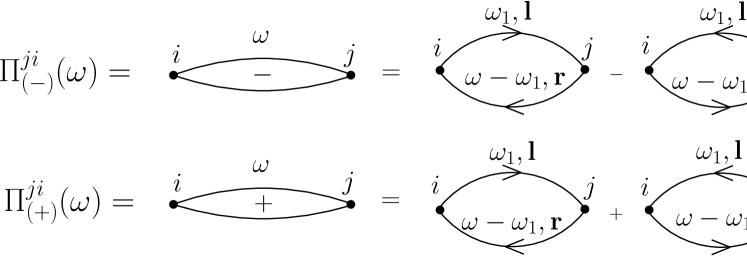
Figure 3: The diagrammatic representation of the junction Green’s functions, Eq. (83). Each bubble represents a linear combination of two electron bubble diagrams, with the Keldysh indices $i$ and $j$. Integration over the internal frequency, $\omega_{1}$, is implicit.

The diagrams with a single oscillator line in Fig. 1 generate sharp features in the noise spectrum at $\omega=\pm\Omega$, while the two-line diagrams in Fig. 2 are responsible for noise peaks in the vicinity of $\omega=0$ and $\omega=\pm 2\Omega$.

An example of a 4-th order diagram whose contribution is a featureless function of frequency $\omega$ is shown in Fig. 4. In this diagram, the frequency of the oscillator line is integrated over and therefore the resonant contribution is absent. Being small compared with the second order contribution to noise, this diagrams and other diagrams of this type can be discarded.

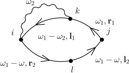
Figure 4: A diagram representing a non-bubble contribution to the noise spectrum. The solid lines represent left and right side electron Green’s function, the wiggly line represents the oscillator Green’s functions. Integration over $\omega_{1}$ and $\omega_{2}$ is implied.

We will denote the resonant contribution of the fourth order diagrams to the current correlator by $S_{res}^{<}$. It is given by the sum

$$S_{res}^{<}(\omega)=S_{v^{2}w^{2}}^{<}(\omega)+S_{w^{4}}^{<}(\omega),$$ (53)

where $S_{v^{2}w^{2}}^{<}(\omega)$ and $S_{w^{4}}^{<}(\omega)$ are the contributions of the diagrams in Fig. 1 and Fig. 2, respectively.

Evaluating the expression represented in Fig. 1 by performing the summation over the contour indices $k$ and $l$, and inserting the bubbles and Green’s functions we get (see Appendix B for details)

$$S_{v^{2}w^{2}}^{<}(\omega)=-2iG_{vw}^{2}VJ(\omega),$$ (54)

where the function $J(\omega)$ is specified in Eq. (34) and the conductance given in Eq. (10). This contribution to the noise spectrum is peaked at $\omega=\pm\Omega$ due to the resonant behavior of the harmonic oscillator spectral function. The dependence of the peak height on the system parameters will be discussed in section IV.3.

The contribution containing two oscillator Green’s functions in Fig. 2 is calculated in Appendix B to give

$$S_{w^{4}}^{<}(\omega) = \frac{G_{ww}^{2}}{2}\int_{-\infty}^{\infty}d\omega_{1}J(\omega_{1})J(\omega-\omega_{1})$$ (55)

$$+ \frac{G_{ww}^{2}}{2}\int_{-\infty}^{\infty}d\omega_{1}A(\omega_{1})A(\omega-\omega_{1})$$

$$\times \left[V-\Delta_{V}(\omega_{1})\right]\left[V-\Delta_{V}(\omega-\omega_{1})\right]$$

where we introduced the oscillator spectral function $A(\omega)=i\left[D^{R}(\omega)-D^{A}(\omega)\right].$ The dependence of the contribution to the noise spectrum, Eq. (55), on system parameters will be discussed in section IV.3.

IV.3 Resonant contributions to the noise spectrum

The resonant contribution to the noise consists of peaks at zero frequency, $\omega=0$, the oscillator frequency, $\omega=\pm\Omega$, and twice the oscillator frequency, $\omega=\pm 2\Omega$. Their heights depend inversely on the damping coefficient of the oscillator, $\gamma$, and their width is proportional to the damping coefficient. In this section we will discuss the properties of the peaked structure and its dependence on environment parameters like bias voltage and temperature. The peaked contribution to the noise can be written as

$$S_{res}^{<}(\omega)=S_{-2}^{<}(\omega)+S_{-1}^{<}(\omega)+S_{0}^{<}(\omega)+S_{1}^{<}(\omega)+S_{2}^{<}(\omega),$$ (56)

where $S_{0}^{<}(\omega)$ describes the peaked contribution to the noise spectrum at zero frequency, $S_{\pm 1}^{<}(\omega)$ the contributions at the oscillator frequency and $S_{\pm 2}^{<}(\omega)$ the contributions at twice the oscillator frequency.

The peaks at the frequencies $\omega=\pm\Omega$ originate from the bubble contribution, $S_{v^{2}w^{2}}^{<}(\omega)$, given in Eq. (54). Inserting the explicit form of the oscillator Green’s functions, Eqs. (17, 22), in Eq. (54), and using that the oscillator Green’s functions are peaked at the oscillator frequency, we obtain for the resonant contribution to the noise spectrum at the oscillator frequency

$$S_{\pm 1}^{<}(\omega)=\frac{\gamma^{2}}{\left(\omega\mp\Omega\right)^{2}+\gamma^{2}}P_{\Omega}.$$ (57)

The peak height at the resonance frequency is

$$P_{\Omega}=\frac{2}{\gamma}\tilde{G}_{vw}^{2}V\left[N^{*}{V}_{+}+\left(N^{*}+1\right){V}_{-}\right],$$ (58)

where ${V}_{\pm}$ is given by Eq. (38) and $N^{*}$ is the occupation number of the oscillator. The peak height scales inversely with the damping coefficient $\gamma$. For large voltages $V\gg\Omega$ the peak height is linear in the occupation number $N^{*}$ and quadratic in the voltage. The result, Eq. (58), extends the result from the Markovian master equation calculation in Refs. CleGir04, ; WabKhoRam05, to voltages smaller than the oscillator frequency.

The peaks at frequencies $\omega=0$ and $\omega=\pm 2\Omega$ come from the fourth order contribution quadratic in the oscillator Green’s functions, Eq. (55). The remaining integration in Eq. (55) can be done and the dominating contribution for weak damping comes from the poles of the oscillator Green’s functions. Collecting the contributions to the peak at zero frequency we get

$$S_{0}^{<}(\omega)=\frac{4\gamma^{2}}{\omega^{2}+4\gamma^{2}}P_{0}$$ (59)

where the peak height $P_{0}$ is

$$P_{0}=\frac{1}{2\gamma}\tilde{G}_{ww}^{2}V\left[N^{*2}{V}_{+}+(N^{*}+1)^{2}{V}_{-}\right].$$ (60)

The peak height at zero frequency also scales inversely with the damping coefficient $\gamma$ and depends quadratically on the conductance $\tilde{G}_{ww}$. The result for the peak at zero frequency, Eq. (59), coincides with the result obtained by using a Markovian master equation approach as in Ref. WabKhoRam05, , which therefore correctly captures the low frequency noise.

The contributions at double the oscillator frequency differ for positive and negative frequency. In the vicinity of $\omega=2\Omega$,

$$S_{2}^{<}(\omega)=\frac{4\gamma^{2}}{\left(\omega-2\Omega\right)^{2}+4\gamma^{2}}P_{2\Omega}$$ (61)

with the peak height given by

$$P_{2\Omega}=\tilde{G}_{ww}^{2}\frac{1}{4\gamma}VN^{*}\left[{V}_{+}N^{*}+{V}_{-}\left(N^{*}+2\right)\right]$$ (62)

and for $\omega\sim-2\Omega$

$$S_{-2}^{<}(\omega)=\frac{4\gamma^{2}}{\left(\omega+2\Omega\right)^{2}+4\gamma^{2}}P_{-2\Omega}$$ (63)

with the peak height

$$P_{-2\Omega} = \tilde{G}_{ww}^{2}\frac{1}{4\gamma}V\left(N^{*}+1\right)$$ (64)

$$\times\left[{V}_{+}\left(N^{*}-1\right)+{V}_{-}\left(N^{*}+1\right)\right].$$

The peaks at double the oscillator frequency also show resonant behavior, i.e. the peak height increases with decreasing damping. For large voltages and occupation number, $N^{*}\gg 1$, it depends quadratically on the oscillator occupation number and the voltage.

The peak heights depend on the bias $V$, the environment temperature $T$ and the relative coupling strengths $\gamma_{e}/\gamma$ and $\gamma_{0}/\gamma$. In the following we discuss the peak heights in some limiting cases.

IV.3.1 Dominant coupling to the tunnel junction

If the coupling between the oscillator and the tunnel junction is much stronger than the coupling to the thermal environment, $\gamma_{e}\gg\gamma_{0}$, the occupation number of the oscillator is, according to Eq. (23), given by

$$N^{*}=\frac{1}{2}\left(\frac{S_{V}(\Omega)}{\Omega}-1\right).$$ (65)

For high temperatures $T\gg V,\Omega$

the occupation number of the oscillator becomes $N^{*}\approx T/\Omega$. The functions ${V}_{\pm}=V$ in this limit. The peak heights of the resonant contributions to the noise spectrum are then at the oscillator frequency

$$P_{\Omega}=\tilde{G}_{vw}^{2}\frac{4}{\gamma}V^{2}\frac{T}{\Omega},$$ (66)

and is linear in the environment temperature. The peak height at zero frequency is

$$P_{0} = \tilde{G}_{ww}^{2}\frac{1}{\gamma}V^{2}\left(\frac{T}{\Omega}\right)^{2},$$ (67)

and depends quadratically on the environment temperature, whereas the peak heights at twice the oscillator frequency become

$$P_{\pm 2\Omega}=\tilde{G}_{ww}^{2}\frac{1}{2\gamma}V^{2}\left(\frac{T}{\Omega}\right)^{2},$$ (68)

which also scales quadratically in the environment temperature. For dominant coupling to the junction $\gamma\propto G_{ww}$ and therefore all the peak heights becomes linear functions of the conductance. The peak heights for high voltages $V\gg T,\Omega$ can be obtained from the peak heights at high temperatures by replacing $T\rightarrow V/2$ in Eqs. (66, 67, 68).

At low temperatures, $T\ll\Omega$,

and low voltages $V<\Omega$, the occupation number approaches zero, $N^{*}\approx 0$. The peaks at the oscillator frequency as well as the peak at zero frequency and the peak at $\omega=2\Omega$ disappear

$$P_{0}=P_{\Omega}=P_{2\Omega}=0.$$ (69)

At $\omega=-2\Omega$ we obtain a dip in the noise spectrum with depth

$$P_{-2\Omega}=-\tilde{G}_{ww}^{2}\frac{1}{2\gamma}V^{2}.$$

Since in nanomechanical systems the coupling strength between the junction and the oscillator can be tuned, we will also discuss the case where the thermal environment dominates over the junction.

IV.3.2 Dominant coupling to the thermal environment

Another limiting case to consider is the situation when the coupling to the thermal environment dominates over the coupling to the tunnel junction, $\gamma_{0}\gg\gamma_{e}$. In the high temperature limit, $T\gg V,\Omega$, we obtain the same results for the peak heights as in the case of dominant coupling to the junction, since for both cases the junction and the thermal environment act as thermal equilibrium environments with temperature $T$. For high voltages and temperatures much larger than the oscillator frequency, $V\gg T\gg\Omega$, we get

$$N^{*}=\frac{\gamma_{e}}{\gamma}\frac{|V|}{2\Omega}+\frac{\gamma_{0}}{\gamma}\frac{T}{\Omega}\gg 1.$$ (70)

The peak height at the oscillator frequency is

$$P_{\Omega}=\tilde{G}_{vw}^{2}\frac{4}{\gamma}V^{2}\left(\frac{\gamma_{e}}{\gamma}\frac{|V|}{2\Omega}+\frac{\gamma_{0}}{\gamma}\frac{T}{\Omega}\right).$$ (71)

The peak height at zero frequency is

$$P_{0}=\tilde{G}_{ww}^{2}\frac{1}{\gamma}V^{2}\left(\frac{\gamma_{e}}{\gamma}\frac{|V|}{2\Omega}+\frac{\gamma_{0}}{\gamma}\frac{T}{\Omega}\right)^{2}.$$ (72)

The peak height at twice the oscillator frequency

$$P_{\pm 2\Omega}=\tilde{G}_{ww}^{2}\frac{1}{2\gamma}V^{2}\left(\frac{\gamma_{e}}{\gamma}\frac{|V|}{2\Omega}+\frac{\gamma_{0}}{\gamma}\frac{T}{\Omega}\right)^{2}$$ (73)

is also quadratic in the occupation number. All peak heights depend inversely on the damping coefficient $\gamma$, since in the parenthesis $\gamma$ appears only in the relative coupling strengths $\gamma_{e}/\gamma$ and $\gamma_{0}/\gamma$.

For low temperatures $T\ll V,\Omega$ we distinguish two regimes. For low voltages, $V<\Omega$, we obtain the same results as in the case for strong coupling to the junction since $N^{*}\approx 0$. For voltages $V\gg\Omega$

$$N^{*}=\frac{\gamma_{e}}{\gamma}\frac{|V|}{2\Omega}.$$ (74)

The functions ${V}_{\pm}\approx V\pm\Omega$ and we obtain for the peak height at the oscillator frequency

$$P_{\Omega}=\tilde{G}_{vw}^{2}\frac{2}{\gamma}V^{2}\left(2\left(\frac{\gamma_{e}}{\gamma}\frac{|V|}{2\Omega}\right)+1\right),$$ (75)

for the peak height at zero frequency

$$P_{0}=\tilde{G}_{ww}^{2}\frac{1}{2\gamma}V^{2}\left[2\left(\frac{\gamma_{e}}{\gamma}\frac{V}{2\Omega}\right)^{2}+2\left(\frac{\gamma_{e}}{\gamma}\frac{|V|}{2\Omega}\right)+1\right]$$ (76)

and the peak heights at twice the oscillator frequency

$$P_{2\Omega}=\tilde{G}_{ww}^{2}\frac{1}{2\gamma}V^{2}\left(\frac{\gamma_{e}}{\gamma}\frac{|V|}{2\Omega}\right)\left[\left(\frac{\gamma_{e}}{\gamma}\frac{|V|}{2\Omega}\right)+1\right]$$ (77)

and

$$P_{-2\Omega}=\tilde{G}_{ww}^{2}\frac{1}{2\gamma}V\left[\left(\frac{\gamma_{e}}{\gamma}\frac{|V|}{2\Omega}\right)+1\right]\left[V\left(\frac{\gamma_{e}}{\gamma}\frac{|V|}{2\Omega}\right)-\Omega\right].$$ (78)

We have obtained the peak heights of the resonant peaks in the noise spectrum of a tunnel junction coupled to a harmonic oscillator for arbitrary parameters $V,\,T$ and $\gamma_{e},\gamma_{0}$. We find that if the oscillator approaches the ground state, $N^{*}\rightarrow 0$, the peaks at positive frequencies as well as the peak at zero vanish. In the next section we are going to discuss an application of the properties of the peaks in the noise spectrum of the junction: noise thermometry.

V Noise Thermometry

In experiments trying to cool a nanomechanical oscillator to the ground state a diagnostic tool is needed to check the state of the oscillator and to confirm, eventually, that the oscillator really is in the ground state. Coupling the oscillator to an electrical device, e.g. a tunnel junction, gives a means to experimentally determine the state of the oscillator, since the oscillator influences the current and noise in the junction. In a noise thermometry setup the noise that the oscillator induces in the tunnel junction is used to determine the temperature or occupation number of the oscillator.

As demonstrated, the noise spectrum of a tunnel junction consists of three peaks, one at zero frequency, one at the oscillator frequency and one at twice the oscillator frequency, and the peak heights depend on the oscillator occupation number. If the oscillator couples weakly to the junction the highest peak is at the oscillator frequency $\Omega$. The relation for the peak height, Eq. (58), can be used to determine the oscillator occupation number in an experiment. The usual experimental procedure (see Refs. NaiBuuLah06, ; LahBuuCam04, ) is to measure the peak height as a function of temperature. Fig. 5 shows the expected outcome of such a measurement, the dependence of the peak height at the oscillator frequency, obtained from Eq. (58), as a function of the environment temperature $T$ for different bias voltages $V$ and dominant coupling to the junction $\gamma_{e}/\gamma=10$. The solid line shows the peak height for $V=0.1\Omega$. It decreases monotonically for decreasing temperature, and becomes exponentially small at low temperatures. The dashed and the dotted line show the peak height for voltages larger than the oscillator frequency ($V=2\Omega$ and $V=5\Omega$ respectively).

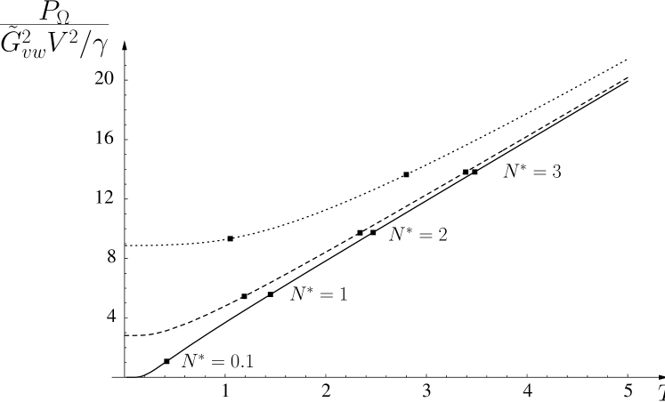
Figure 5: The peak height of the noise at the oscillator frequency, $P_{\Omega}$, as a function of the environment temperature $T$ for different bias voltages and dominant coupling to the junction, $\gamma_{e}/\gamma_{0}=10$, and $\tilde{G}_{vw}=0.1$. The full line shows the temperature dependence of the peak height for $V=0.1\Omega$, the dashed line for $V=2\Omega$ and the dotted line for $V=5\Omega$. As the environment temperature approaches zero, the peak height vanishes for voltages $V<\Omega$, but stays finite for voltages $V>\Omega$. The square dots mark different occupation numbers of the oscillator as indicated.

The height of the peak $P_{\Omega}$ can be conveniently scaled to a dimensionless quantity $N_{c}$,

$$N_{c}=\gamma\frac{P_{\Omega}}{4\tilde{G}_{vw}^{2}V^{2}},$$ (79)

where the combination $\gamma/\tilde{G}_{vw}^{2}$ is a property of the device. For high occupation numbers (i.e. high temperatures or high voltage, $\max(V,T)\gg\Omega$), the dimensionless peak height $N_{c}$ gives the oscillator occupation number: $N^{*}\approx N_{c}$. The normalization constant, $4\tilde{G}_{vw}^{2}V^{2}/\gamma$ in Eq. (79 ), can be read off as the high temperature slope in a plot of $P_{\Omega}$ vs. $T/\Omega$. In the region of low occupation numbers we obtain the relation for the occupation number

$$N^{*}=N_{c}-\frac{1}{2}\frac{{V}_{-}}{V}.$$ (80)

where ${V}_{-}$, Eq. (38), is a known function of the bias and temperature.

We note that for low temperatures and voltages the oscillator occupation number is not simply proportional to the peak height at the oscillator frequency. The relative occupation number $N^{*}/N_{c}$ is shown in Fig. 6 for dominant coupling to the junction and different bias voltages. At high temperatures the relative occupation number approaches unity, for low temperatures and low voltages it departs from unity.

Figure 6: The relative occupation number of the oscillator $N^{*}/N_{c}$ as a function of the environment temperature $T$ for different bias voltages $V$ and dominant coupling to the junction, $\gamma_{e}/\gamma_{0}=10$, with $\tilde{G}_{vw}=0.1$. The full line shows the relative occupation number for low voltage, $V=0.1\Omega$, the dashed line and the dotted line show the relative occupation number for high voltages, $V=2\Omega$ and $V=5\Omega$, respectively. For high temperatures $T\gg\Omega$, the relative occupation number approaches unity. For low temperatures the relative occupation number can depart considerably from unity to approach $1/(1+\gamma\Omega/\gamma_{e}V)$.

Another possibility to get information on the oscillator occupation number is from the peak heights at $\omega=0$ and $\omega=2\Omega$ using Eqs. (60, 62). The combination of junction parameters $V^{2}\tilde{G}_{ww}^{2}/\gamma$ in Eqs. (60, 62) can be obtained, e.g, from the high temperature slope in a plot of $P_{0}$ vs. $T^{2}/\Omega^{2}$.

Since the peak at the oscillator frequency is not isolated, but sits on a noise floor, the question of observability of the peak arises. As a measure of observability we define a signal to noise ratio, the peak height relative to the floor

$$r=\frac{P_{\Omega}}{S_{vv}(\Omega)+S_{ww}(\Omega)},$$ (81)

and demand $r>0.1$ for the peak to be observable. The peak height, $P_{\Omega}$, as well as the magnitude of the noise floor, $S_{vv}(\Omega)+S_{ww}(\Omega)$, depend on $N^{*}$, the junction bias, and the junction temperature as well as the conductances $G_{vv},\,\tilde{G}_{vw}$ and $\tilde{G}_{ww}$. To investigate the observability of the peak, we use Eq. (81) to find the occupation number $N^{*}$ for a given bias voltage, junction temperature and a set of conductances, so that $r=0.2$. The solid lines in Fig. 7 show the occupation number necessary to fulfill $r=0.1$ as a function of voltage and junction temperature. To detect an oscillator close to its ground state high bias voltages and / or low junction temperatures are necessary, as seen in Fig. 7. On the other hand, high voltages heat the oscillator, so that a compromise between heating and readout has to be found. To illustrate the heating effect, the dash-dotted lines show the occupation number for dominant coupling to the junction, $\gamma_{e}/\gamma_{0}=100$. If one would like to read out the oscillator occupation number when $N^{*}<0.1$, without introducing heating, voltage and temperature are confined to the shaded region on the left of Fig. 7. This example shows that a good signal to noise ratio for the readout and a minimal heating of the oscillator are complimentary requirements.

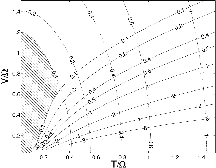
Figure 7: The solid lines show are a contour plot of the minimum occupation number necessary to observe the peak at the oscillator frequency with a S/N ratio $r>0.2$, as a function of voltage and temperature with relative conductances $G_{vv}/\tilde{G}_{vw}=10$ and $G_{ww}/\tilde{G}_{vw}=0.1$ . The dashed lines are a contour plot of the occupation number of the oscillator for dominant coupling to the junction, $\gamma_{e}/\gamma_{0}=100$. The shaded region to the left marks the parameter regime that allows a readout of the oscillator occupation number without heating the oscillator.

VI Conclusion

We have considered a nanomechanical resonator interacting with a dc-biased tunnel junction. We model the resonator as a harmonic oscillator and the interaction is introduced via the modulation of the tunneling amplitude by coupling to the harmonic oscillator position. Employing a Green’s function technique we calculated the properties of the stationary state of the oscillator, obtaining that the coupling to the junction introduces damping and heats the oscillator. The expression Eq. (23), for the temperature of a harmonic oscillator coupled to a tunnel junction was also obtained in Ref. WabKhoRam05, using a Markovian master equation approach. The reason for the coinciding results derived by two different techniques is due to the same weak coupling approximation made in both derivations. Both, the perturbative Green’s function calculation presented here and the Markovian master equation can only be applied for weak coupling between the environment and the oscillator. In the master equation approach the weak coupling leads to a separation of time scales of the environment evolution and the evolution of the density matrix, resulting in a Markovian master equation. Here the same argument is used in the frequency domain: The width of the oscillator spectral function is small on the scale of the frequency dependence of the environment correlation functions.

The current-voltage characteristic of the junction has been obtained. The stationary state current is seen to consist of two contributions. One contribution is the current through an isolated junction, whereas the other contribution, dependent on the state of the oscillator, stems from oscillator assisted tunneling. The expression obtained for the dc-current is in accordance with the result previously derived using a master equation technique.WabKhoRam05 ; bum The additional current arising from the influence of the oscillator on the junction transmission, Eq. (36), vanishes if the oscillator is in the ground state and the voltage across the junction is smaller than the oscillator frequency. We observe therefore that the zero point fluctuations of the oscillator position do not affect the electric current.

The main part of the paper presents the calculation of the electric noise due to oscillator-assisted tunnelling. The unsymmetrized current-current correlator has been evaluated for arbitrary frequencies, bias voltages, and environment temperatures. The noise spectrum consists of a smooth noise floor and a peaked resonant structure.

As a function of frequency $\omega$, the noise floor varies on the scale $\max(T,V,\Omega)$. The contribution of the oscillator is shown to vanish at positive frequencies when the oscillator is in the ground state and the bias voltage is smaller than the oscillator frequency. The expressions Eqs. (47, 52) for the second order noise generalize the result obtained by a Markovian master equation derived in Ref. WabKhoRam05, . In the Markovian master equation calculation a constant noise floor was obtained, whereas the Green’s function calculation presented here captures the frequency dependent noise floor. As expected, in the low frequency limit, we recover the result obtained by the Markovian master equation approach.

The resonant structure in the noise spectrum, $S^{<}(\omega)$, consists of peaks at zero frequency, $\omega=0$, the oscillator frequency, $\omega=\pm\Omega$, and twice the oscillator frequency, $\omega=\pm 2\Omega$. Being present only for a finite voltage across the junction, the resonances are of non-equilibrium origin, and their intensities at positive and negative frequencies are not related by the detailed balance relation. GavLevImr00 The peaks at the oscillator frequency have the same height for positive and negative frequencies, whereas the peaks at double the oscillator frequency are asymmetric. The peaks at $\omega=\pm\Omega$ stem from processes involving a single vibrational quantum, and their height is therefore linear in the oscillator occupation number $N^{*}$, whereas the processes leading to the peaks at $\omega=0$ and $\omega=\pm 2\Omega$ involve two quanta and the peak heights are quadratic in $N^{*}$. If the oscillator is in the ground state, the peaks at positive frequencies vanish in the limit where the bias voltage is smaller than the oscillator frequency but a dip in the noise spectrum remains for negative frequencies.

For bias voltages smaller than the oscillator frequency and the oscillator in the ground state, we find no oscillator dependent noise at positive frequencies: Both the oscillator dependent contribution to the noise floor as well as the peaks at positive frequencies disappear from the unsymmetrized noise spectrum, $S^{<}(\omega)$. The oscillator contribution to the current-current correlator at negative frequencies remains finite even for voltages smaller than the oscillator frequency.

To understand this result we consider a setup for measuring current fluctuations. Lesovik and LoosenLesLoo97 as well as Gavish, Levinson and Imry,GavLevImr00 introduced a damped harmonic oscillator with resonance frequency $\Omega_{0}$ as a meter of current fluctuations. For linear coupling of the oscillator to the current in the junction, they obtained the deviation of the meter position fluctuations, $\langle X^{2}\rangle$, from the equilibrium value in terms of the current-current correlators of the junction, $S^{<}$ and $S^{>}$ (see Eq. (29)), and the meter occupation number, $N_{\Omega_{0}}$,

$$\delta\left\langle\hat{X}^{2}\right\rangle=A\left[\left(N_{\Omega_{0}}+1\right)S^{<}(\Omega_{0})+N_{\Omega_{0}}S^{>}(\Omega_{0})\right],$$ (82)

where $A$ is the coupling strength and $N_{\Omega_{0}}$ is the Bose function with temperature $T$. Note that the argument of the noise spectrum $S^{<,>}$, the oscillator frequency $\Omega_{0}$ is positive. Let us consider the meter fluctuations in different temperature ranges. For large detector temperatures $T\gg\Omega_{0}$, and consequently $N_{\Omega_{0}}\gg 1$, the meter fluctuations are proportional to the symmetrized current-current correlator of the junction, $S^{>}+S^{<}$. A passive detector – a detector at low temperature $T\ll\Omega_{0}$, when $N_{\Omega_{0}}\ll 1$ – measures the unsymmetrized current-current correlator $S^{<}$ at positive frequency. In accordance with these arguments,LesLoo97 ; GavLevImr00 only the part of $S^{<}$ at positive frequencies describes physical noise, understood as random flow of energy from the system to environment.

We can now understand our results for the current-current correlator $S^{<}(\omega)$ with the help of Eq. (82). A passive detector detects only the positive frequency part of the current-current correlator. Our calculations show vanishing $S^{<}(\omega)$ at positive frequencies $\omega$ in the case when the oscillator is in the ground state, and thus the ground state does not contribute to the physical noise in the tunnel junction in compliance with general expectations.

In experiments with nanomechanical resonators utilizing electrical devices as detectors, noise properties can function as a diagnostic tool in determining the state of the resonator. We have shown how peaks in the noise power spectrum can act as a measure for the oscillator occupation number and discussed the criteria for observing these peaks.

In this paper we presented a calculation of the noise induced by an oscillator in a tunnel junction. The obtained results are valid at arbitrary parameters and thus also in the important region where the oscillator approaches the ground state.

Appendix A Junction Green’s functions

In this section we are going to calculate the junction Green’s functions that appeared in the calculation of the properties of the oscillator stationary state, the average current and the noise. The junction Green’s functions encountered are

$$\Pi_{uu^{\prime}}^{+}(\tau_{1},\tau_{2}) = -i\left\langle\mathrm{T}_{c}\left(h_{u}(\tau_{1})h_{u^{\prime}}(\tau_{2})\right)\right\rangle,$$

$$\Pi_{uu^{\prime}}^{-}(\tau_{1},\tau_{2}) = -\left\langle\mathrm{T}_{c}\left(h_{u}(\tau_{1})j_{u^{\prime}}(\tau_{2})\right)\right\rangle,$$ (83)

where the notation was introduced in section II, and the contour times discussed in section III. In terms of the tunneling operators $\mathcal{T}$ and $\mathcal{T}^{\dagger}$, Eq. (3), taken in the interaction picture, we have

$$\Pi_{uu^{\prime}}^{{\pm}}(\tau_{1},\tau_{2}) = -i\left[\left\langle\mathrm{T}_{c}\left(\mathcal{T}_{u}(\tau_{1})\mathcal{T}_{u^{\prime}}^{\dagger}(\tau_{2})\right)\right\rangle\right.$$ (84)

$$\pm \left.\left\langle\mathrm{T}_{c}\left(\mathcal{T}_{u}^{\dagger}(\tau_{1})\mathcal{T}_{u^{\prime}}(\tau_{2})\right)\right\rangle\right].$$

Inserting the tunneling operator from Eq. (7) we get the symmetric and antisymmetric combinations of left and right electrode electron Green’s functions

$$\Pi_{uu^{\prime}}^{{\pm}}(\tau_{1},\tau_{2}) = -i\sum_{\mathbf{lr}}u_{\mathbf{lr}}u^{\prime}_{\mathbf{rl}}\left[G_{\mathbf{l}}(\tau_{2}-\tau_{1})G_{\mathbf{r}}(\tau_{1}-\tau_{2})\right.$$ (85)

$$\quad\quad\left.\pm G_{\mathbf{r}}(\tau_{2}-\tau_{1})G_{\mathbf{l}}(\tau_{1}-\tau_{2})\right],$$

where we introduced the electron Green’s function for the right and left electrodes, for example

$$G_{\mathbf{l}}(\tau_{1},\tau_{2})=-i\left\langle\mathrm{T}_{c}\left(c_{\mathbf{l}}(\tau_{1})c_{\mathbf{l}}^{\dagger}(\tau_{2})\right)\right\rangle.$$ (86)

The Green’s functions of interest can be obtained by standard techniques. For example,

$$\Pi_{uu^{\prime}\pm}^{<}(t_{1},t_{2})=-i\left[\left\langle\mathcal{T}_{u^{\prime}}^{\dagger}(t_{2})\mathcal{T}_{u}(t_{1})\right\rangle\pm\left\langle\mathcal{T}_{u^{\prime}}(t_{2})\mathcal{T}_{u}^{\dagger}(t_{1})\right\rangle\right],$$

is given in terms of its Fourier transform

$$\Pi_{uu^{\prime}\pm}^{<}(\omega) = -2\pi i\sum_{\mathbf{lr}}u_{\mathbf{lr}}u^{\prime}_{\mathbf{rl}}\left[f(\epsilon_{\mathbf{l}})-f(\epsilon_{\mathbf{r}})\right]$$ (87)

$$\times\left\{\left[1+n(\epsilon_{\mathbf{r}}-\epsilon_{\mathbf{l}})\right]\delta(\epsilon_{\mathbf{r}}-\epsilon_{\mathbf{l}}+V-\omega)\right.$$

$$\pm\left.n(\epsilon_{\mathbf{r}}-\epsilon_{\mathbf{l}})\delta(\epsilon_{\mathbf{r}}-\epsilon_{\mathbf{l}}+V+\omega)\right\},$$

where $n(\omega)$ is the Bose function. For voltages $V\ll E_{F}$ we obtain the approximate relation

$$\sum_{\mathbf{lr}}u_{\mathbf{lr}}u^{\prime}_{\mathbf{rl}}\left[f(\epsilon_{\mathbf{l}})-f(\epsilon_{\mathbf{r}})\right]\delta(\epsilon_{\mathbf{r}}-\epsilon_{\mathbf{l}}+V)$$

$$=V\,\sum_{\mathbf{lr}}u_{\mathbf{lr}}u^{\prime}_{\mathbf{rl}}\left(-\frac{\partial f(\epsilon_{\mathbf{l}})}{\partial\epsilon_{\mathbf{l}}}\right)\delta(\epsilon_{\mathbf{r}}-\epsilon_{\mathbf{l}}),$$ (88)

as tunneling amplitudes depend only weakly on their arguments, so that

$$\Pi_{uu^{\prime}\pm}^{<}(\omega) = iG_{uu^{\prime}}\left[\left(V-\omega\right)\left[1+n(V-\omega)\right]\right.$$

$$\left.\pm\left(V+\omega\right)n(V+\omega)\right]$$

where we introduced the conductance

$$G_{uu^{\prime}}=2\pi\sum_{\mathbf{lr}}u_{\mathbf{lr}}u^{\prime}_{\mathbf{rl}}\left(-\frac{\partial f(\epsilon_{\mathbf{l}})}{\partial\epsilon_{\mathbf{l}}}\right)\delta(\epsilon_{\mathbf{r}}-\epsilon_{\mathbf{l}}).$$ (89)

The retarded, advanced and Keldysh bubbles

$$\Pi_{{uu^{\prime}\pm}}^{R}(t_{1}-t_{2}) = -i\theta(t_{1}-t_{2})\left[\left\langle\left[\mathcal{T}_{u}(t_{1}),\mathcal{T}_{u^{\prime}}^{\dagger}(t_{2})\right]\right\rangle\right.$$

$$\left.\pm\left\langle\left[\mathcal{T}_{u}^{\dagger}(t_{1}),\mathcal{T}_{u^{\prime}}(t_{2})\right]\right\rangle\right]$$

$$\Pi_{{uu^{\prime}\pm}}^{A}(t_{1}-t_{2}) = -i\theta(t_{2}-t_{1})\left[\left\langle\left[\mathcal{T}_{u}(t_{1}),\mathcal{T}_{u^{\prime}}^{\dagger}(t_{2})\right]\right\rangle\right.$$

$$\left.\pm\left\langle\left[\mathcal{T}_{u}^{\dagger}(t_{1}),\mathcal{T}_{u^{\prime}}(t_{2})\right]\right\rangle\right]$$

$$\Pi_{{uu^{\prime}\pm}}^{K}(t_{1}-t_{2}) = -i\left[\left\langle\left\{\mathcal{T}_{u}(t_{1}),\mathcal{T}_{u^{\prime}}^{\dagger}(t_{2})\right\}\right\rangle\right.$$ (90)

$$\left.\pm\left\langle\left\{\mathcal{T}_{u}^{\dagger}(t_{1}),\mathcal{T}_{u^{\prime}}(t_{2})\right\}\right\rangle\right]$$

can be calculated in a similar way to give

$$\Pi_{uu^{\prime}}^{-}(\omega)=-i\left(\begin{array}[]{cc}\Pi_{-}^{R}(\omega)&\Pi_{-}^{K}(\omega)\\ 0&\Pi_{-}^{A}(\omega)\end{array}\right)_{uu^{\prime}}$$ (91)

with

$$\Pi_{uu^{\prime}-}^{R}(\omega) = -iG_{uu^{\prime}}V+R_{uu^{\prime}}^{-}(\omega)$$

$$\Pi_{uu^{\prime}-}^{K}(\omega) = -2iG_{uu^{\prime}}\Delta_{V}(\omega)$$ (92)

and the advanced part given by $\Pi_{-}^{A}(\omega)=\left[\Pi_{-}^{A}(\omega)\right]^{*}$, with the functions $S_{V}(\omega)$ and $\Delta_{V}(\omega)$ defined in Eqs. (16, 35) respectively, and similarly $\Pi_{uu^{\prime}}^{+}(\omega)$ is given by Eq. (15).

The real parts of the retarded $\Pi_{uu^{\prime}}^{\pm}(\omega)$ are given by

$$R_{uu^{\prime}}^{\pm}(\omega)=2\pi\sum_{\mathbf{lr}}u_{\mathbf{lr}}u^{\prime}_{\mathbf{rl}}\left[f(\epsilon_{\mathbf{l}})-f(\epsilon_{\mathbf{r}})\right]\left(P_{-}\pm P_{+}\right)$$ (93)

with $P_{\pm}=1/(\epsilon_{\mathbf{l}}-\epsilon_{\mathbf{r}}\pm V+\omega).$ To estimate the real parts, we ignore the weak energy dependence of the transmission amplitudes and the electron density of states are constants up to a cut-off frequency of the order of the Fermi energy $E_{F}$. For frequencies and voltages much smaller than the cutoff frequency, $\omega,V\ll E_{F}$, we can approximate the reactive parts of the response functions Eq. (93) to give

$$R_{uu^{\prime}}^{-}(\omega) \sim G_{uu^{\prime}}V\frac{\omega}{E_{F}}$$

$$R_{uu^{\prime}}^{+}(\omega) \sim G_{uu^{\prime}}E_{F}.$$ (94)

This concludes our calculation of the junction Green’s functions.

Appendix B Fourth order diagrams

In this appendix we give the algebraic expressions for the fourth order diagrams contributing to the current-current correlator. Let us consider, for example, the contribution containing bubbles that is linear in the oscillator Green’s function, i.e., the diagrams depicted in Fig. 1

$$S_{v^{2}w^{2}}^{<}(\omega) = -i\sum_{kl}s^{kl}\left(\Pi_{-}^{l1}(\omega)\Pi_{-}^{k2}(\omega)D^{kl}(\omega)\right.$$ (95)

$$+\Pi_{-}^{l1}(0)\Pi_{-}^{k2}(0)D^{12}(\omega)$$

$$+\Pi_{-}^{l1}(\omega)\Pi_{-}^{k2}(0)D^{k2}(\omega)$$

$$\left.+\Pi_{-}^{l1}(0)\Pi_{-}^{k2}(\omega)D^{k1}(\omega)\right),$$

where the full oscillator Green’s function appears, accounting for the influence of the interaction with the tunnel junction and the matrix

$$s^{kl}=\left(\begin{array}[]{cc}1&-1\\ -1&1\end{array}\right)$$ (96)

introduces the correct signs for forward and backward contour (to simplify notation, we suppress subscripts $v$ and $w$ on the right hand side). Performing the summation over the contour indices $k$ and $l$, and inserting the bubbles and Green’s functions we obtain Eq. (54).

Similarly, the contribution from diagrams containing two oscillator Green’s functions, see Fig. 2, becomes

$$S_{w^{4}}^{<}(\omega) = \sum_{kl}s^{kl}\int d\omega_{1}\Lambda^{kl}(\omega,\omega_{1}),$$ (97)

$$\Lambda^{kl}(\omega,\omega_{1}) = \Pi_{-}^{l1}(\omega_{1})\Pi_{-}^{k2}(\omega_{1})D^{kl}(\omega_{1})D^{21}(\omega-\omega_{1})$$

$$+ \Pi_{-}^{l1}(\omega-\omega_{1})\Pi_{-}^{k2}(\omega_{1})D^{2l}(\omega-\omega_{1})D^{k1}(\omega_{1}).$$

Doing the summation and inserting the bubbles and oscillator Green’s functions we obtain Eq. (55), where we neglected a non-resonant contribution that is small compared to the second order contributions to the noise floor, Eqs. (52, 47).

All diagrams not containing bubbles are of the non-resonant kind, i.e. oscillator Green’s functions always appear under frequency integration. A typical non-bubble contribution to the noise spectrum is shown in Fig. 4 and given by

$$\bar{s}_{v^{2}w^{2}}^{<}(\omega)=\int d\omega_{1}d\omega_{2}\sum_{kl}s^{kl}\sum_{\mathbf{l}_{1}\mathbf{r}_{1}}\sum_{\mathbf{l}_{2}\mathbf{r}_{2}}v^{2}w^{2}G_{\mathbf{l}_{1}}^{1k}(\omega_{1}-\omega_{2})G_{\mathbf{l}_{2}}^{2l}(\omega_{1}-\omega)G_{\mathbf{r}_{1}}^{k2}(\omega_{1})G_{\mathbf{r}_{2}}^{l1}(\omega_{1}-\omega)D^{k1}(\omega_{2}).$$ (98)

Since there are no resonant peaks present, contributions of this type have to be compared to the second order contribution to the noise floor, Eqs. (47, 52) and since they are always of higher order in tunneling they can be neglected.

References

- (1) K. C. Schwab and M. L. Roukes, Physics Today, July 2005, 37 (2005).
- (2) M. Blencowe, Phys. Rep. 395, 159 (2004).
- (3) K. L. Ekinci and M. L. Roukes, Review of Scientific Instruments 76, 061101 (2005).
- (4) V. Sazonova, Y. Yaish, H. Üstünel, D. Roundy, T. A. Arias and P. L. McEuen, Nature 431, 284 (2004).
- (5) A. J. Leggett, J. Phys.: Condens. Matter 14, R415-R451 (2002).
- (6) W. Marshall, C. Simon, R. Penrose and D. Bouwmeester, Phys. Rev. Lett. 91, 130401 (2003).
- (7) A. Naik, O. Buu, M. D. LaHaye, A. D. Armour, A. A. Clerk, M. P. Blencowe and K. C. Schwab, Nature 443, 193 (2006).
- (8) M. D. LaHaye, O. Buu, B. Camarota and K. C. Schwab, Science 304, 74 (2004).
- (9) S. Gigan, H. R. Böhm, M. Paternostro, F. Blaser, G. Langer, J. B. Hertzberg, K. C. Schwab, D. Bäuerle, M. Aspelmeyer and A. Zeilinger, Nature 444, 67 (2006).
- (10) O. Arcizet, P.-F. Cohandon, T. Briant, M. Pinard, and A. Heidmann, Nature 444, 71 (2006).
- (11) D. Kleckner and D. Bouwmeester, Nature 444, 75 (2006).
- (12) Y. T. Yang, C. Callegari, X. L. Feng, K. L. Ekinci and M. L. Roukes, Nano Letters 6, 583 (2006).
- (13) D. Rugar, R. Budakian, H. J. Mamin and B. W. Chu, Nature 430, 329-332 (2004).
- (14) M. R. Geller and A. N. Cleland, Phys. Rev. A 71, 032311 (2005).
- (15) D. Mozyrsky and I. Martin, Phys. Rev. Lett. 89, 018301 (2002).
- (16) A. A. Clerk and S. M. Girvin, Phys. Rev. 70, 121303 (2004).
- (17) J. Wabnig, D. V. Khomitsky, J. Rammer and A. L. Shelankov, Phys. Rev. B 72, 165347 (2005).
- (18) A. Yu. Smirnov, L. G. Mourokh and N. J. M. Horing, Phys. Rev. B 67, 115312 (2003).
- (19) D. A. Rodrigues and A. D. Armour, Phys. Rev. B 72, 085324 (2005).
- (20) M. P. Blencowe, J. Imbers and A. D. Armour, New Journal of Physics 7, 236 (2005).
- (21) A. A. Clerk and S. Bennett, New Journal of Physics 7, 238 (2005).
- (22) L. Spietz, K. W. Lehnert, I. Siddiqi and R. J. Schoelkopf, Science 300, 1929 (2003).
- (23) Xin-Qi Li, Ping Cui and Yi Jing Yan, Phys. Rev. Lett. 94, 066803 (2005).
- (24) G. B. Lesovik and R. Loosen, JETP Lett. 65, 295 (1997).
- (25) R. Aguado and L. P. Kouwenhoven, Phys. Rev. Lett. 84, 1986 (2000).
- (26) U. Gavish, Y. Levinson and Y. Imry, Phys. Rev. B 62, R10637 (2000).
- (27) J. Rammer and H. Smith, Rev. Mod. Phys. 58, 323 (1986).
- (28) Sh. Kogan, Electronic noise and fluctuations in solids, Cambridge University Press, (1996).
- (29) A. A. Clerk, Phys. Rev. B 70, 245306 (2004).
- (30) A. J. Dahm, A. Denenstein, D. N. Langenberg, W. H. Parker, D. Rogovin and D. J. Scalapino, Phys. Rev. Lett. 22, 1416 (1969).
- (31) The additional pumping contribution to the current found in Ref. WabKhoRam05, is not present here, since for simplicity we take the junction to be symmetric implying real transmission matrix elements.