A transition from river networks to scale-free networks

Abstract

A spatial network is constructed on a two dimensional space where the nodes are geometrical points located at randomly distributed positions which are labeled sequentially in increasing order of one of their co-ordinates. Starting with $N$ such points the network is grown by including them one by one according to the serial number into the growing network. The $t$-th point is attached to the $i$-th node of the network using the probability: $\pi_{i}(t)\sim k_{i}(t)\ell_{ti}^{\alpha}$ where $k_{i}(t)$ is the degree of the $i$-th node and $\ell_{ti}$ is the Euclidean distance between the points $t$ and $i$. Here $\alpha$ is a continuously tunable parameter and while for $\alpha=0$ one gets the simple Barabási-Albert network, the case for $\alpha\to-\infty$ corresponds to the spatially continuous version of the well known Scheidegger’s river network problem. The modulating parameter $\alpha$ is tuned to study the transition between the two different critical behaviors at a specific value $\alpha_{c}$ which we numerically estimate to be -2.

Scale-free networks (SFN) are highly inhomogeneous with a power law decay of their nodal degree distributions signifying the absence of a characteristic value for the nodal degrees barabasi . Extensive research over last several years revealed that such networks indeed occur in different real-world systems like protein interaction networks in Biology, Internet and World-wide web (WWW) in electronic communication systems, airport networks in public transport systems etc. barabasireview ; Dorogovtsev ; Romuldo . On the other hand, river networks are relatively simple spatial networks which were being studied over last several decades from the geological point of view. During the last decade or so physicists have also studied properties of river networks with many different simple model networks mainly from the interests generated about their fractal properties, a popular topic of critical phenomena Rinaldo .

In this paper we report our study of an weighted spatial network on the two-dimensional plane. The weight of a link is evidently the Euclidean length of the link. Tuning a parameter which modulates the strength of the contribution of the link weight in the attachment probability, we are able to obtain networks similar to the directed river network model in one limit. On the other limit of the parameter we obtain scale-free networks. The transition point for the crossover between the two types of behaviors is studied.

The simplest river network model on a lattice is the Scheidegger’s river network with a directional bias Scheidegger . This is simply described on an oriented square lattice: Each lattice site is associated with an outgoing arrow representing the direction of the flow vector from that site. Only two possible choices for this arrow are possible: it may direct to the lower left lattice site or to the lower right. An independent and uncorrelated assignment of an arrow from each site results a ‘Directed Spanning Tree’ (DST) network network ; Rahul . Such networks are characterized mainly by the critical exponents associated with the distributions of the river basin area as well as the length of the longest river at each site. The set of associated exponents constitute the universality class of the Scheidegger’s river network which are different from the similar exponents of the isotropic spanning tree networks Manna-Dhar-Majum .

On the other hand while studying the scale-free properties of different real-world networks Barabási and Albert (BA) argued that there is a ‘Rich get richer’ mechanism in-built with the growth process of every SFN barabasi . They proposed a model of generating scale-free networks where new nodes are introduced to the growing network at a rate of one per unit time step which are connected with the growing network with $m$ distinct links with a probability proportional to the individual nodal degree: $\pi_{i}(t)\propto k_{i}(t)$ barabasi . Also there are some other directed scale-free networks whose links are meaningful only when there is a connection from one end to the other but not along the reverse direction, e.g., the World-wide web web , the phone-call network phone and the citation network Redner etc.

Real-world networks whose nodes are geographically located in different positions on a two-dimensional Euclidean space are very important in their own right. For example the electrical networks in power transmissions, railway or postal networks in transport networks are few of the very well known spatial networks. Research over last few years have also revealed that two very important spatial networks like the Internet Faloutsos ; Pastor ; Yook and the Airport networks Guimera ; Barrat have scale-free structures.

Weighted networks are those whose links are associated with non-uniform weights $w_{ij}$. Therefore the spatial networks are by definition weighted networks whose link weights are the Euclidean lengths of the links. For a weighted network one can define the strength of a node $i$ as the total sum of the weights $s_{i}=\Sigma_{j}w_{ij}$. How the average nodal strength $\langle s(k)\rangle$ varies with the degree $k$, i.e., $\langle s(k)\rangle\propto k^{\beta}$ is also a non-trivial question. Non-linear strength-degree relations have been observed for the Internet as well as the Airport networks. In this context a detailed knowledge of link length distribution is also important e.g., in the study of Internet’s topological structure for designing efficient routing protocols and modeling Internet traffic. Early studies like the Waxman model describes the Internet with exponentially decaying link length distribution Waxman . Yook et. al. observed that nodes of the router level network maps of North America are distributed on a fractal set and the link length distribution is inversely proportional to the link lengths Yook . A number of model networks on the Euclidean space have been studied in different contexts Rozenfeld ; Manna-Sen .

Figure 1: Pictures of the network generated for the four different values of the modulating parameter $\alpha$ using the same set of $N=1024$ randomly distributed points within the unit square box. Link lengths are large for $\alpha=0$ which gradually shrink in length as $\alpha$ decreases and the network becomes the directed minimal spanning tree at $\alpha=-\infty$.

We consider here a stack of nodes dropped one by one on a substrate with increasing vertical co-ordinates. Each node is connected randomly with a specific link length dependent probability of attachment to a node of the already grown stack.

A network of $N$ nodes is grown within an unit square box on the two-dimensional $x-y$ plane. Nodes are represented by $N$ points selected at random positions ${(x_{i},y_{i})},i=1,N$ by generating their values from an uniform probability distribution $\{0,1\}$. The first point is placed by hand at the bottom of the box with $y_{1}=0$. All other points are assigned serial numbers in increasing order of their $y$-coordinates: $y_{1}<y_{2}<y_{3}...<y_{N}$. We use the geometry of a cylinder i.e., impose the open boundary condition along the $y$-direction but the periodic boundary condition along the $x$-direction. This implies that the space is continuous along the $x$-direction and any node very close to the $x=1$ line may have a right neighbor inside the box and very close to the line $x=0$ and vice-versa.

To start with we assume that the first node at the bottom of the box has a ‘pseudo’ degree $k_{1}=1$. Then the nodes from 2 to $N$ are connected to the network by one link each. The time $t$ measures the growth of the network by the number of nodes. The $t$-th node is then linked to the growing network with an attachment probability

$$\pi_{i}(t)\propto k_{i}(t)\ell_{ti}^{\alpha}$$ (1)

where $\ell_{ti}$ denotes the Euclidean distance between the $t$-th and the $i$-th nodes maintaining the periodic boundary condition. This implies that the attachment probability has two competing factors. The linear dependence on the degree $k_{i}(t)$ enhances the probability of connection to a higher degree node where as the factor $\ell^{\alpha}$ reduces the probability of selection when $\alpha>0$ and enhances when $\alpha<0$. The special case of $\alpha=0$ the attachment probability in Eqn. (1) clearly corresponds to the Barabási-Albert model. We now discuss the properties of the network by continuously tuning the parameter $\alpha$ through its accessible range.

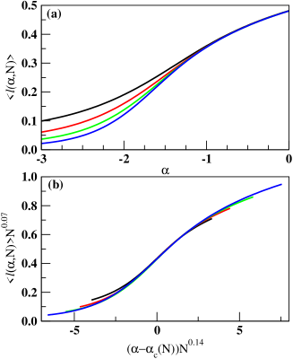
Figure 2: (Color online) The average length of a link $\langle\ell(\alpha,N)\rangle$ has been plotted in (a) with the continuously tunable parameter $\alpha$ for different values of the system sizes: $N=2^{8},2^{10},2^{12}$ and $2^{14}$. $N$ increases from top to bottom. In (b) a scaling is shown with the system size dependent critical value of $\alpha_{c}$ which approaches -2 as $N\to\infty$.

In the limit of $\alpha\to-\infty$ every node connects its nearest node $i$ in the downward direction corresponding to the smallest value of the link length $\ell$ with probability one irrespective of its degree $k_{i}$ and therefore the probability of attachment to any other node is identically zero. This link may be directed either to the left or to the right depending on the position of the nearest node (Fig. 1).

Let us first study the first neighbor distance distribution. Consider an arbitrary point P at an arbitrary position. The probability that its first neighbor is positioned on the semi-annular ring within $r$ and $r+dr$ in the downward direction (which can be done in $N-1$ different ways) and all other $N-2$ points are at distances larger than $r+dr$ is:

$${\rm Prob}(r,N)dr=(N-1)\hskip 2.84544pt\pi rdr\hskip 2.84544pt(1-\pi r^{2}/2)^{N-2}.$$ (2)

In the limit of $N\to\infty$ it can be approximated that $N-1\approx N-2\approx N$ and since the average area per point decreases as $1/N$, $\pi r^{2}/2$ is very small compared to 1. Therefore $(1-\pi r^{2}/2)^{N-2}$ is approximated as $\exp(-\pi Nr^{2}/2)$. In the limit of $N\to\infty$ the probability density distribution is therefore:

$${\rm Prob}(r,N)=\pi Nr\hskip 2.84544pt\exp(-\pi Nr^{2}/2)$$ (3)

or in the scaling form:

$$\frac{1}{\sqrt{N}}{\rm Prob}(r) = [\pi r\sqrt{N}]\hskip 2.84544pt\exp(-\pi[r\sqrt{N}]^{2}/2)={\cal G}(x)$$ (4)

where the scaling function ${\cal G}(x)=\pi x\exp(-\pi x^{2}/2)$ and $x=r\sqrt{N}$. Numerical results for the link length distribution of different system sizes verifies this distribution very accurately.

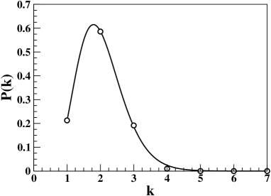
Figure 3: The degree probability distribution $P(k)$ vs. $k$ of the network in the limit of $\alpha\to-\infty$ and for $N=2^{18}$. The solid line is a fit and its functional form is given in Eqn. (7).

The typical length $\langle\ell(\alpha,N)\rangle$ of a link for a network of size $N$ and generated with a specific value of the parameter $\alpha$ is estimated by averaging the link length over all $N-1$ links of a network as well as over many independent configurations. For this purpose one can define a total cost function ${\cal C}(\alpha,N)$ of the network which is the total length of all the links:

$${\cal C}(\alpha,N)=\Sigma_{j=1}^{N-1}\ell_{j}\hskip 2.84544pt{\rm and}\hskip 2.84544pt\langle\ell(\alpha,N)\rangle={\cal C}(\alpha,N)/(N-1).$$ (5)

In Fig. 2(a) we show the variation of the average link length with $\alpha$. The $\langle\ell(\alpha,N)\rangle\to 0$ as $\alpha\to-\infty$ and gradually increases with increasing $\alpha$. Around $\alpha_{c}=-2$ the $\langle\ell(\alpha,N)\rangle$ increases very fast and finally approaches unity as $\alpha\to+\infty$. The steep growth around $\alpha_{c}$ becomes increasingly sharper with increasing system size. For very large networks $N\to\infty$ it appears that for $\alpha<\alpha_{c}$ $\langle\ell(\alpha,N)\rangle\to 0$ and for $\alpha>\alpha_{c}$ it approaches a finite value. Such a system size dependence is quantified by a finite-size scaling of this plot as shown in Fig. 2(b). The data collapse shows that

$$\langle\ell(\alpha,N)\rangle\propto N^{-0.07}{\cal G}[(\alpha-\alpha_{c}(N))N^{0.14}].$$ (6)

The critical values of $\alpha_{c}(N)$ for a system of size $N$ is located at the value of $\alpha$ where $\langle\ell(\alpha,N)\rangle$ increased most rapidly with $\alpha$. The values of $\alpha_{c}(N)$ so obtained are $-1.37$, -1.46. -1.54 and -1.60 for $N=2^{8},2^{10},2^{12}$ and $2^{14}$ and are extrapolated with $N^{-0.1}$ to get $\alpha_{c}=\alpha_{c}(\infty)=-2.0\pm 0.10$. Similar results of $\alpha_{c}=-2$ have been obtained in Kleinberg ; Roberson .

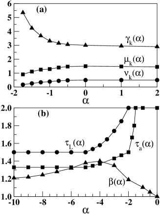
Figure 4: (a) Variation of the scaling exponents $\nu_{k}(\alpha)$, $\mu_{k}(\alpha)$ and $\gamma_{k}(\alpha)$ characterizing the degree distribution in Eqn. (8) with the modulating parameter $\alpha$. (b) Variation of the exponents $\tau_{a}(\alpha)$, $\tau_{L}(\alpha)$ and $\beta(\alpha)$ with $\alpha$.

In the limit of $\alpha\to-\infty$ and $N\to\infty$, the fractions of nodes with degrees 1, 2 and 3 are found to be 0.213, 0.586 and 0.192 respectively and decreases very fast for higher degree values. The whole distribution fits nicely to a sharp Gamma distribution as (Fig. 3):

$$P(k)\propto k^{7.5}\exp(-4.2k).$$ (7)

In the range $\alpha>\alpha_{c}$ we observed that the network has a scale-free structure. For large system sizes the degree distribution follows a power law like $P(k)\propto k^{-\gamma}$ but for finite systems a finite-size scaling seems to work well:

$${\rm Prob}(k,N)\propto N^{-\mu_{k}}{\cal F}_{k}(k/N^{\nu_{k}}).$$ (8)

The scaling function ${\cal F}_{k}(x)\sim x^{-\gamma_{k}}$ for $x\to 0$ and decreases faster than a power law for $x>>1$ so that, $\gamma_{k}=\mu_{k}/\nu_{k}$. For a range of $\alpha$ values the scaling exponents are measured and it is observed that all three exponents $\gamma_{k},\mu_{k}$ and $\nu_{k}$ are dependent on the value of $\alpha$ (Fig. 4(a)).

For the river network problems the size of the drainage area is a popular quantity to measure. The amount of water that flows out of a node of the river network is proportional to the area whose water is drained out through this node. On a tree network the drainage area $a_{i}$ is defined at every node $i$ and is measured by the number of nodes supported by $i$ on the tree network. A well known recursion relation for $a_{i}$ is: $a_{i}=\Sigma_{j}a_{j}\delta_{ij}+1$ where the dummy index $j$ runs over the neighboring nodes of $i$ and $\delta_{ij}=1$ if the flow direction is from $j$ to $i$, otherwise it is zero. The probability distribution ${\rm Prob}(a)$ of the drainage areas is the probability that a randomly selected node has the area value $a$. It is known that for river networks this distribution has a power law variation: ${\rm Prob}(a)\sim a^{-\tau_{a}}$ Rinaldo .

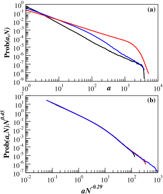
Figure 5: (Color online) Plot of the river basin area $a$ distribution in our model for different network sizes $N$. In (a) ${\rm Prob}(a,N)$ has been shown for three different values of $\alpha$: $\alpha=-\infty$ at the top, $\alpha=\alpha_{c}$ at the middle and $\alpha=0$ at the bottom. In (b) a finite size scaling of ${\rm Prob}(a,N)$ with $N$ has been shown for $\alpha=\alpha_{c}$ for $N=2^{8},2^{9}$ and $2^{10}$.

The drainage area distribution is measured first in the limit of $\alpha\to-\infty$ for our networks of different sizes $N=2^{12},2^{14}$ and $2^{16}$. Direct measurement of the slopes of double logarithmic plots of ${\rm Prob}(a,N)$ vs. $a$ gives values of the exponent $\tau\approx 1.33$ which varied little with the system size (Fig. 5(a)). This estimate is consistent with that obtained from the finite size scaling analysis. An excellent scaling of the data over different system sizes is obtained as:

$${\rm Prob}(a,N)\propto N^{-\mu_{a}}{\cal F}(a/N^{\nu_{a}})$$ (9)

and the exponent $\tau_{a}=\mu_{a}/\nu_{a}$. In the limit of $\alpha\to-\infty$ we estimated $\mu_{a}(-\infty)\approx 1.00$ and $\nu_{a}(-\infty)\approx 0.75$ giving a value for the exponent $\tau_{a}(-\infty)\approx 1.33$. These values are very much consistent with the same exponents of Scheidegger’s river network model where $\tau_{a}=4/3$ is known exactly Scheidegger . Similarly for $\alpha=0$ we could reproduce the known values of $\mu_{a}(0)\approx 2.00$ and $\nu_{a}(0)\approx 1.00$ with $\tau_{a}(0)\approx 2.00$ as obtained in Redner . Finally we measured the same distribution at the transition point $\alpha_{c}=-2$ and obtained $\mu_{a}(-2)\approx 0.45$ and $\nu_{a}(2)\approx 0.29$ with $\tau_{a}(-2)\approx 1.50$ (Fig. 5(b)).

Another quantity of interest is the length $L_{i}$ of the longest up-stream meeting at the node $i$. It’s magnitude is the number of links on the longest path terminating at $i$. ${\rm Prob}(L)$ therefore denotes the probability that an arbitrarily selected node $i$ has $L_{i}=L$. Given a network of size $N$, $L$ values are measured at every node and then the data is sampled over many uncorrelated network configurations and for different network sizes. A similar finite size scaling form like ${\rm Prob}(L,N)\propto N^{-\mu_{L}}{\cal G}(L/N^{\nu_{L}})$ works here as well. We obtain $\mu_{L}(-\infty)\approx 0.75$, $\nu_{L}(-\infty)\approx 0.50$, $\tau_{L}(-\infty)=1.5$ and $\mu_{L}(2)\approx 0.2$, $\nu_{L}(2)\approx 0.1$, $\tau_{L}(2)\approx 2.0$.

Finally, we studied the strength-degree relation in our model. Here the weight of a link is the length of the link $\ell_{ij}$ and therefore the strength of the node $i$ is $s_{i}=\Sigma_{j}\ell_{ij}$. The strength $\langle s(k)\rangle$ per node averaged over all nodes of degree $k$ of the network as well as over many independent realizations varies with the degree $k$ as: $\langle s(k,\alpha)\rangle\propto k^{\beta(\alpha)}$. Numerically we observe that the exponent $\beta(\alpha)$ varies with the tuning parameter $\alpha$. Fig. 4(b) summarizes the variation of the three exponents $\tau_{a}(\alpha)$, $\tau_{L}(\alpha)$ and $\beta(\alpha)$ within the range of $\alpha$ varying between -10 and 0. For $\alpha\leq-5$, $\tau_{a}(\alpha)$ and $\tau_{L}(\alpha)$ values coincide with their values at $\alpha=-\infty$. Between $-5<\alpha\leq-2$, $\tau_{L}(\alpha)$ slowly increases to 2 and $\tau_{a}(\alpha)$ increases to 1.5.

To conclude, we have defined and studied a network embedded in the Euclidean space. Random distribution of nodes are sequentially numbered in increasing heights and the degree dependent attachment probability is modulated by the $\alpha$-th power of the link length. This continuously tunable parameter $\alpha$ interpolates between the Scheidegger’s river network and the Barabasi-Albert Scale-free network. It appears that there exists a critical value $\alpha_{c}$ such that for $\alpha<\alpha_{c}$ the critical behavior of the network is like the Scheidegger’s river network, whereas for $\alpha>\alpha_{c}$ critical exponents are indistinguishable from those of ordinary BA network. Our numerical study indicates $\alpha_{c}$ is likely to be -2.

Discussion with G. Mukherjee and K. Bhattacharya are thankfully acknowledged.

Electronic Address: manna@bose.res.in

References

- (1) A.-L. Barabási and R. Albert, Science, 286, 509 (1999).
- (2) R. Albert and A.-L. Barabási, Rev. Mod. Phys. 74, 47 (2002).
- (3) S. N. Dorogovtsev and J. F. F. Mendes, Evolution of Networks, Oxford University Press, 2003; M. E. J. Newman, SIAM Review 45, 167 (2003).
- (4) R. Pastor-Satorras and A. Vespignani, Evolution and Structure of the Internet, A Statistical Physics Approach, Cambridge University Press, 2004.
- (5) I. Rodríguez-Iturbe, A. Rinaldo, Fractal River Basins: Chance and Self-Organization, Cambridge University Press, 2001.
- (6) A.E. Scheidegger, Geol. Soc. Am. Bull. 72, 37 (1961); Water Resour. Res. 4, 167 (1968).
- (7) F. Harary, Graph Theory, Addison-Wesley Publishing Company, Inc., Reading, Mass., 1969.
- (8) A. G. Bhatt and R. Roy, Appl. Probab. 36, 19 (2004).
- (9) S. S. Manna, D. Dhar and S. N. Majumdar, Phys. Rev. A. 46 R4471 (1992).
- (10) S. Lawrence and C. L. Giles, Science, 280, 98 (1998); Nature, 400, 107 (1999), R. Albert, H. Jeong and A.-L. Barabási, Nature, 401, 130 (1999).
- (11) W. Aiello, F. Chung and L. Lu in Proc. 32-nd ACM Symp. Theor. Comp. (2000).
- (12) P. L. Krapivsky and S. Redner, Phys. Rev. E. 63, 066123 (2001).
- (13) M. Faloutsos, P. Faloutsos and C. Faloutsos, Proc. ACM SIGCOMM, Comput. Commun. Rev., 29, 251 (1999).
- (14) R. Pastor-Satorras, A. Vazquez and A. Vespignani, Phys. Rev. Lett. 87, 258701 (2001).
- (15) S. H. Yook, H. Jeong and A.-L. Barabási, Proc. Natl. Acad. Sci. (USA) 99, 13382 (2002).
- (16) R. Guimera and L. A. N. Amaral, Eur. Phys. Jour. B, 38, 381 (2004).
- (17) A. Barrat, M. Barthélémy, R. Pastor-Satorras, A. Vespignani, Proc. Natl. Acad. Sci. (USA), 101, 3747 (2004).
- (18) B. Waxman, IEEE J. Selec. Areas Commun., SAC, 6, 1617 (1988).
- (19) A. F. Rozenfeld, R. Cohen, D. b-Avraham and S. Havlin, Phys. Rev. Lett. 89, 218701 (2002).
- (20) S. S. Manna and P. Sen, Phys. Rev. E 66, 066114 (2002).
- (21) J. M. Kleinberg, Nature, 406, 845 (2000).
- (22) M. R. Roberson and D. ben-Avraham, Phys. Rev. E 74, 017101 (2006).