Excitable Greenberg-Hastings cellular automaton model on scale-free networks

Abstract

We study the excitable Greenberg-Hastings cellular automaton model on scale-free networks. We obtained analytical expressions for no external stimulus and the uncoupled case. It is found that the curves, the average activity $F$ versus the external stimulus rate $r$, can be fitted by a Hill function, but not exactly, and there exists a relation $F\propto r^{\alpha}$ for the low-stimulus response, where Stevens-Hill exponent $\alpha$ ranges from $\alpha=1$ in the subcritical regime to $\alpha=0.5$ at criticality. At the critical point, the range reaches the maximal. We also calculate the average activity $F^{k}(r)$ and the dynamic range $\Delta^{k}(p)$ for nodes with given connectivity $k$. It is interesting that nodes with larger connectivity have larger optimal range, which could be applied in biological experiments to reveal the network topology.

Many systems in the real world, either naturally evolved or artificially designed, are organized in a network fashion Albert . The most studied networks are the exponential networks in which the nodes’ connectivity distribution (the probability $P(k)$ that a node if connected to other k nodes) is exponentially bounded. A typical model of this network is the Watts-Strogatz (WS) graph Watts which exhibits the “small-world”phenomenon that was observed in realistic networks Watts_1 . On the contrary, it has been observed recently that the nodes’ degree distribution of many networks have power-law tails (scale-free property, due to the absence of a characteristic value for the degrees) $P(k)\sim k^{-\gamma}$ with $2\leq\gamma\leq 3$ Barabasi .

Scale-free (SF) networks have been widely studied in the past few years, mainly because of their connection to a lot of real-world structures, including networks in nature, such as the cell, metabolic networks and the food web, artificial networks such as the Internet and the WWW, or even social networks, such as sexual partnership networks Albert . The SF network is characterized with the power-law degree distribution. Thus there always exists a small number of nodes which are connected to a large number of other nodes in SF networks. This heterogeneity leads to intriguing properties of SF networks. A lot of work has been devoted in the literature to the study of static properties of the networks, while many interests are growing for dynamical properties on these kind of networks. In the context of percolation, SF networks are stable against random removal of nodes while they are fragile under intentional attacks targeting on nodes with high degree Albert2 ; Cohen . Also, there are absences of epidemic thresholds in SF networks Pastor and of the kinetic effects in reaction-diffusion processes taking place on SF networks GA04 .

In this paper, we will study the excitable Greenberg-Hastings cellular automaton (GHCA) model Greenberg78 on the SF network, especially we focus here on the Barabási and Albert (BA) graph Barabasi . Due to experimental data which suggest that some classes of spiking neurons in the first layers of sensory systems are electrically coupled via gap junctions or ephaptic interactions, the GHCA model is employed to model the response of the sensory network to external stimuli in some recent works. Two-dimensional deterministic cellular automaton model was studied by computer simulations Copelli05 . Analytical results have recently been obtained for the one-dimensional cellular automaton model under the two-site mean-field approximation Furtado06 . In ref. Kinouchi , Kinouchi and Copelli studied the GHCA model on Erdös-Rényi random graph with stochastic activity propagation, and they found a new and important result that dynamic range maximized at the critical point, which is perhaps the first clear example of signal processing optimization at a phase transition.

In the $n$-state GHCA model Greenberg78 for excitable systems, the instantaneous membrane potential of the $i$-th cell ($i=1,\ldots,N$) at discrete time $t$ is represented by $x_{i}(t)\in\{0,1,\ldots,n-1\}$, $n\geq 3$. The state $x_{i}(t)=0$ denotes a neuron at its resting (polarized) potential, $x_{i}(t)=1$ represents a spiking (depolarizing) neuron and $x_{i}(t)=2,\ldots,n-1$ account for the afterspike refractory period (hyperpolarization). There are two ways for the $i$-th element to go from state $x_{i}(t)=0$ to $x_{i}(t+1)=1$: a) due to an external signal, modelled here by a Poisson process with rate $r$ (which implies a transition with probability $\lambda=1-\exp(-r\Delta t)$ per time step); b) with probability $p$, due to a neighbor $j$ being in the excited state in the previous time step. If $x_{i}(t)\geq 1$, then $x_{i}(t+1)=(x_{i}(t)+1)\text{mod }n$, regardless of the stimulus. In other words, the rules state that a neuron only spikes if stimulated, after which it undergoes an absolute refractory period before returning to rest. Time is discrete. We assume $\Delta t=1$ ms which corresponds to the approximate duration of a spike and is the time scale adopted for the time step of the model. The number of states $n$ therefore controls the duration of the refractory period (which corresponds to $n-2$, in ms). In the biological context, $r$ could be related for example with the concentration of a given odorant presented to an olfactory epithelium Rospars00 , or the light intensity stimulating a retina Deans02 . We shall refer to $r$ as the stimulus rate or intensity.

BA graph is a kind of SF networks and can be constructed according to ref. Barabasi . Starting from a small number $m_{0}$ of nodes, every time step a new vertex is added, with $m$ links that are connected to an old node $i$ with probability $\Pi_{i}=k_{i}/\sum_{j}k_{j}$, where $k_{i}$ is the connectivity of the $i$th node. After iterating this scheme a sufficient number of times, we obtain a network composed by $N$ nodes with connectivity distribution $P(k)\sim k^{-3}$ and average connectivity $\langle k\rangle=2m$. For this kind network, the absence of a characteristic scale for the connectivity makes highly connected nodes statistically significant, and induces strong fluctuations in the connectivity distribution which cannot be neglected.

Let $\rho_{t}(s)$ be the densities of neurons which are in state $s$ at time $t$. We have the normalization condition, $\sum_{s=0}^{n-1}\rho_{t}(s)=1$. Since the dynamics of the refractory state is deterministic, the equations for $s\geq 2$ are simply

$$\rho_{t+1}(2) = \rho_{t}(1)$$

$$\rho_{t+1}(3) = \rho_{t}(2)$$

$$\vdots$$

$$\rho_{t+1}(n-1) = \rho_{t}(n-2)\;.$$ (1)

By imposing the stationarity condition, we have

$$\rho_{t}(0)=1-(n-1)\rho_{t}(1),$$ (2)

Following ideas developed by Pastor-Satorras et al. Pastor , to take into account strong fluctuations in the connectivity distribution, we consider the relative density $\rho_{t}{{}^{k}}(1)$ of active nodes with given connectivity $k$ by the following equation

$$\partial_{t}\rho_{t}{{}^{k}}(1)=-\rho_{t}{{}^{k}}(1)+\lambda\rho_{t}{{}^{k}}(0)+kp(1-\lambda)\rho_{t}{{}^{k}}(0)\Theta(\rho_{t}(1)),$$ (3)

where $\Theta(\rho_{t}(1))$ is the probability that any given link point to an active node and is assumed as a function of the total density of exciting nodes $\rho_{t}(1)$. In the steady state, $\rho_{t}(1)$ is just a function of $\lambda$ and $p$. Thus, the probability $\Theta$ becomes an implicit function of $\lambda$ and $p$. By imposing the stationarity condition, $\partial_{t}\rho_{t}{{}^{k}}(1)=0$, we obtain

$$\rho{{}^{k}}(1)=\frac{\lambda+(1-\lambda)pk\Theta(\lambda,p)}{1+(n-1)[\lambda+(1-\lambda)pk\Theta(\lambda,p)]}.$$ (4)

This set of equations show that the higher the node connectivity, the higher the probability to be in a spiking state. This inhomogeneity must be taken into account in the computation of $\Theta(\lambda,p)$. Indeed, the probability that a link points to a node with $q$ links is proportional to $qP(q)$. In other words, a randomly chosen link is more likely to be connected to an exciting node with high connectivity, yielding the relation

$$\Theta(\lambda,p)=\sum_{k}\frac{kP(k)\rho{{}^{k}}(1)}{\sum_{q}qP(q)}.$$ (5)

Since $\rho{{}^{k}}(1)$ is on its turn a function of $\Theta(\lambda,p)$, we obtain a self-consistency equation that allows to find $\Theta(\lambda,p)$ and an explicit form for Eq. (4). Finally, we can evaluate the order parameter (persistence) $\rho(1)$ using the relation

$$\rho(1)=\sum_{k}P(k)\rho{{}^{k}}(1).$$ (6)

For the BA graph, the full connectivity distribution is given by $P(k)=2m^{2}k^{-3}$, where $m$ is the minimum number of connection at each node. By noticing that the average connectivity is $\langle k\rangle=\int_{m}^{\infty}kP(k)dk=2m$, Eq. (5) gives

$$\Theta(\lambda,p)=m\int_{m}^{\infty}\frac{1}{k^{2}}\frac{\lambda+(1-\lambda)pk\Theta(\lambda,p)}{1+(n-1)[\lambda+(1-\lambda)pk\Theta(\lambda,p)]},$$ (7)

which yields the solution

$$\Theta(\lambda,p)=\frac{\lambda}{b}+(\frac{\lambda}{b}-\frac{1}{n-1})\frac{ma\Theta(\lambda,p)}{b}\ln\frac{ma\Theta(\lambda,p)}{ma\Theta(\lambda,p)+b},$$ (8)

where $a=(n-1)(1-\lambda)p$ and $b=1+(n-1)\lambda$. We can solve the above equation to obtain the solution $\Theta(\lambda,p)$. Theoretically, combing Eqs. (4) , (6) and (8), we can obtain the final result of $\rho(1)$. In some special cases the analytical expressions can be obtained.

i) no external stimulus, i.e., $\lambda=0$ or $r=0$. We can obtain

$$\Theta(0,p)=\frac{e^{-1/mp}}{(n-1)mp}(1-e^{-1/mp})^{-1}.$$ (9)

Combing Eqs. (4), (6), and (9), we find the solution of the density of active nodes when there is no external stimulus,

$$\rho(1)\sim\frac{1}{n-1}e^{-1/mp}.$$ (10)

ii) the uncoupled case, i.e., $p=0$. Combing Eqs. (4) and (6), we have

$$\rho(1)=\frac{\lambda}{1+(n-1)\lambda},$$ (11)

which is independent of the network’s topology, so it is also have been obtained in other networks, such as one dimensional case Furtado06 . When the external stimulus intensity $r$ is very small, $\rho(1)\sim r^{-1}$.

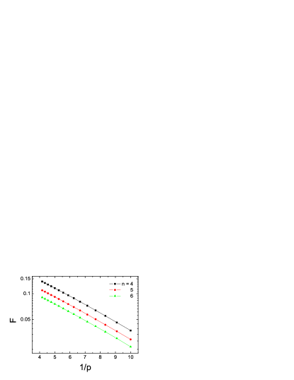
Figure 1: In the absence of stimulus, the average activity $F$ as a function of $1/p$ for BA networks of size $N=10^{4}$ and $m_{0}=m=4$. The linear behavior on the semi-logarithmic scale proves an exponential behavior predicted by Eq. (10).

We define the average activity

$$F=\frac{1}{T}\sum_{t=1}^{T}\rho_{t}(1),$$ (12)

where $T$ is a large time window (of the order of $10^{4}$ time steps). In the stationary state, it is obviously that $F=\rho(1)$. To confirm the picture extracted from the above analytic treatment, we perform numerical simulations on the BA network. Figure 1 shows the behavior of the average activity $F$ in the absence of stimulus. All the plots decays with an exponent form $F\sim\exp(-c/mp)$, where $c$ is a constant. The numerical value obtained $c=0.226$ is in good agreement with the theoretical prediction $c=1/m=0.25$.

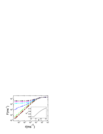
Figure 2: Response curves (mean firing rate vs. stimulus rate). Points represent simulation results with $N=10^{4}$, $m_{0}=m=4$, $n=5$ states and $T=10^{3}$ ms, from $p=0$ to $p=0.12$ (in intervals of 0.02). These curves are power laws $F\propto r^{\alpha}$ with $\alpha=1$ (subcritical) and $\alpha=1/2$ (critical). Inset: spontaneous activity $F_{0}$ vs. branching probability $p$, the critical point is $p_{c}=0.06$.

In Fig. 2, we show the average activity $F$ versus the external stimulus rate $r$ for different branching probability $p$. The inset shows the spontaneous activity $F_{0}$ versus the branching probability $p$ in the absence of stimulus ($r=0$), there is a critical point $p_{c}=0.06$, only at $p>p_{c}$ there is a self-sustained activity, $F>0$. The curves $F(r)$ could be fitted by a Hill function, but are not exactly Hill, and there exists the relation $F\propto r^{\alpha}$ for the low-stimulus response. It is found that the Stevens-Hill exponent $\alpha$ changes from $\alpha=1$ in the subcritical regime to $\alpha=0.5$ at criticality. This important point was also reported by ref. Kinouchi where the network is an Erdös-Rényi random graph. We also notice that apparent exponents between 0.5 and 1.0 are observed Furtado06 if finite size effects are present, that is, if $N$ is small.

Figure 3: Dynamic range vs. branching probability $p$. The curve is obtained by calculating the data from Fig.2. In the subcritical regime, the dynamic range $\Delta(p)$ increases monotonically with $p$, In the supercritical regime, $\Delta(p)$ decreases when $p$ increases. There is a maximal range precisely at the critical point $p_{c}=0.06$.

As a function of the stimulus intensity $r$, networks have a minimum response $F_{0}$ (= 0 for the subcritical and critical cases) and a maximum response $F_{max}$ (due to the absolute nature of the refractory period, $F_{max}=1/n$, which can be obtained by setting $\lambda=1$ in Eqs. (11)). Ref. Kinouchi defines the dynamic range $\Delta=10\log(r_{0.9}/r_{0.1})$ as the stimulus interval (measured in dB) where variations in $r$ can be robustly coded by variations in $F$, discarding stimuli which are too weak to be distinguished from $F_{0}$ or too close to saturation. The range $[r_{0.1},r_{0.9}]$ is found from its corresponding response interval $[F_{0.1},F_{0.9}]$, where $F_{x}=F_{0}+x(F_{max}-F_{0})$.

Figure 3 depicts the dynamic range $\Delta$ versus the branching probability $p$. In the subcritical regime, the dynamic range $\Delta(p)$ increases monotonically with $p$, In the supercritical regime, $\Delta(p)$ decreases when $p$ increases. There is a maximal range precisely at the critical point. This result was also found in Erdös-Rényi random graph Kinouchi . Kinouchi and Copelli explained the result as “In the subcritical regime, sensitivity is enlarged because weak stimuli are amplified due to activity propagation among neighbours. As a result, the dynamic range $\Delta(p)$ increases monotonically with $p$. In the supercritical regime, the spontaneous activity $F_{0}$ masks the presence of weak stimuli, therefore $\Delta(p)$ decreases. The optimal regime occurs precisely at the critical point”Kinouchi . We also perform simulations on other complex networks, such as WS networks and random SF networks with different $\gamma$, and obtain the same behavior of the average activity $F$ as it is shown in Fig. 2, the optimal regime occuring precisely at the critical point. We state that this phenomenon is the universal behavior of excitable GHCA model on complex networks and the explanation provided by Kinouchi and Copelli is also suitable for other types of complex networks.

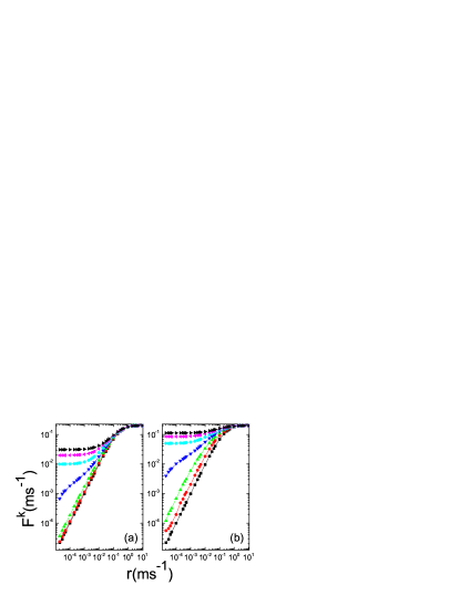
Figure 4: Average activity $F^{k}$ for nodes with given connectivity $k$ vs. external stimulus rate $r$. (a) for connectivity $k=4$, and (b) for connectivity $k=36$. Simulations are performed with $N=10^{4}$, $m_{0}=m=4$, $n=5$ states and $T=10^{4}$ ms, from $p=0$ to $p=0.12$ (in intervals of 0.02). These curves are power laws $F^{k}\propto r^{\alpha}$ with $\alpha=1$ (subcritical) and $\alpha=1/2$ (critical).

In SF networks, there exist strong fluctuations in the connectivity distribution. It is worthy to investigate the behavior of the average activity $F^{k}$ for nodes with given connectivity $k$. In Fig. 4 we plot the quantity $F^{k}$ versus the external stimulus intensity $r$ for different branching probability $p$. Figs. 4(a) and (b) correspond to the node’s connectivity $k=4$ and $36$, respectively. It is found that the curves $F^{k}(r)$ have the similar property of $F(r)$ which was shown in Fig. 2, i.e., the Stevens-Hill exponent $\alpha$ changes from $\alpha=1$ in the subcritical regime to $\alpha=0.5$ at criticality.

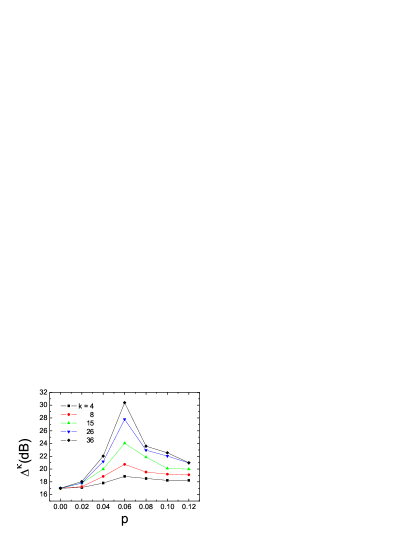
Figure 5: Dynamic range $\Delta^{k}(p)$ of nodes with given connectivity $k$ vs. branching probability $p$. Points represent the results calculated from simulation with $N=10^{4}$ sites, $m_{0}=m=4$, $n=5$ states and $T=10^{4}$ ms. Dynamic range $\Delta^{k}(p)$ is optimized at the critical point $p_{c}=0.06$, although the connectivity $k$ is different .

Finally, we calculate the dynamic range $\Delta^{k}(p)$ of nodes with given connectivity $k$, and the result is shown in Fig. 5. The phenomenon that the optimal regime occurs precisely at the critical point recurs. It is notable that the optimal dynamic range for nodes with given connectivity $k$ increases with $k$, i.e., for the node with larger connectivity, its corresponding larger optimal range. One can investigate every node’s optimal dynamic range and calculate their fluctuations, since the fluctuations of node’s optimal dynamic range reflect the fluctuations of the node’s connectivity in the network. To some extent, we can discovery the topology of the network by investigating the dynamics on it.

In summary, we have investigated the behavior of the excitable GHCA model Greenberg78 on BA networks. We found out that the curves of the average activity $F$ as a function of the external stimulus rate $r$ can be fitted by a Hill function, but are not exactly Hill, and there exists a relation $F\propto r^{\alpha}$ for the low-stimulus response. The Stevens-Hill exponent $\alpha$ changes from $\alpha=1$ in the subcritical regime to $\alpha=0.5$ at criticality. There is a maximal range precisely at the critical point. We also observed these results numerically in other kind of complex networks. We conclude that these phenomena are the universal behaviors of the excitable GHCA model on complex networks. Due to strong fluctuations in the connectivity distribution on the BA graph, we calculated the average activity $F^{k}(r)$ and the dynamic range $\Delta^{k}(p)$ for nodes with given connectivity $k$. The two quantities $F^{k}(r)$ and $\Delta^{k}(p)$ have the similar behavior as that of $F(r)$ and $\Delta(p)$, respectively. It is interesting that nodes with larger connectivity have larger optimal range. This property could be applied in biological experiment revealing the network topology.

This work was supported by the Fundamental Research Fund for Physics and Mathematics of Lanzhou University under Grant No. Lzu05008. X.-J. Xu acknowledges financial support from FCT (Portugal), Grant No. SFRH/BPD/30425/2006.

References

- (1) R. Albert and A.-L. Barabási, Rev. Mod. Phys. 74, 47 (2002); S.N. Dorogovtsev and J.F.F. Mendes, Adv. Phys. 51, 1079 (2002); M.E.J. Newman, SIAM Rev. 45, 167 (2003).
- (2) D.J. Watts and S.H. Strogatz, Nature 393, 440 (1998).
- (3) D.J. Watts, Small Worlds: The Dynamics of Networks Between Order and Randomness (Princeton University Press, New Jersey, 1999).
- (4) A.-L. Barabási and R. Albert, Science 286, 509 (1999); A.-L. Barabási, R. Albert, and H. Jeong, Physica A 272, 173 (1999).
- (5) R. Albert, H, Jeong, and A.-L. Barabási, Nature (London) 406, 378 (2000).
- (6) R. Cohen, K. Erez, D. ben-Avraham, and S. Havlin, Phys. Rev. Lett. 85, 4626 (2000).
- (7) R. Pastor-Satorras and A. Vespignani, Phys. Rev. Lett. 86, 3200 (2001); Phys. Rev. E 63, 066117 (2001); ibid 65, 036104 (2002).
- (8) L.K. Gallos and P. Argyrakis, Phys. Rev. Lett. 92, 138301 (2004).
- (9) J.M. Greenberg and S.P. Hastings, SIAM J. Appl. Math. 34, 515 1978.
- (10) M. Copelli and O. Kinouchi, Physica A 349, 431 (2005).
- (11) L.S. Furtado and M. Copelli, Phys. Rev. E 73, 011907 (2006).
- (12) O. Kinouchi and M. Copelli, Nat. Phys. 2, 348 (2006).
- (13) J.-P. Rospars, P. Lánský, P. Duchamp-Viret, and A. Duchamp, BioSystems 58, 133 (2000).
- (14) M.R. Deans, B. Volgyi, D.A. Goodenough, S.A. Bloomfield, and D.L. Paul, Neuron 36, 703 (2002).