Morphological stability of electromigration-driven vacancy islands

Abstract

The electromigration-induced shape evolution of two-dimensional vacancy islands on a crystal surface is studied using a continuum approach. We consider the regime where mass transport is restricted to terrace diffusion in the interior of the island. In the limit of fast attachment/detachment kinetics a circle translating at constant velocity is a stationary solution of the problem. In contrast to earlier work [O. Pierre-Louis and T.L. Einstein, Phys. Rev. B 62, 13697 (2000)] we show that the circular solution remains linearly stable for arbitrarily large driving forces. The numerical solution of the full nonlinear problem nevertheless reveals a fingering instability at the trailing end of the island, which develops from finite amplitude perturbations and eventually leads to pinch-off. Relaxing the condition of instantaneous attachment/detachment kinetics, we obtain non-circular elongated stationary shapes in an analytic approximation which compares favorably to the full numerical solution.

I Introduction

Much of the diversity of natural shapes in the inanimate world is the result of morphological instabilities. The paradigmatic example is the Mullins-Sekerka instability, in which a spherical solid nucleus in an undercooled melt forms lobes and petals which eventually develop into a delicate dendritic pattern Pelcé (2004), and its two-dimensional analogs that can be observed in the growth of islands on crystal surfaces Michely and Krug (2004). These systems share the common mathematical structure of moving boundary value problems, in which an interface evolves in response to the gradient of some continuous field defined in the spatial domains that it separates. In the context of two-dimensional crystal surfaces, the interfaces are atomic height steps separating different terraces, and their motion is governed by the attachment and detachment of the adsorbed atoms (adatoms) Jeong and Williams (1999); Pierre-Louis (2005); Krug (2005).

A rich variety of two-dimensional morphological instabilities has been observed on the surfaces of current-carrying crystals, where an electromigration force induces a directed motion of adatoms Yagi et al. (2001); Minoda (2003). The microscopic origin of this force is a combination of momentum transfer from the conduction electrons (the ’wind force’) and a direct effect of the local electric field Sorbello (1998). On stepped surfaces vicinal to Si(111), electromigration has been found to cause step bunching Latyshev et al. (1989), step meandering Degawa et al. (1999), step bending Thürmer et al. (1999) and step pairing Pierre-Louis and Métois (2004) instabilities. In addition, single layer adatom islands on silicon surfaces have been seen to drift under the influence of electromigration Métois et al. (1999); Saúl et al. (2002).

In the present paper we focus on the morphological stability of single layer vacancy islands driven by electromigration. We build on the work of Pierre-Louis and Einstein (PLE) Pierre-Louis and Einstein (2000), who introduced a class of continuum models for island electromigration. The different models are distinguished according to the dominant mechanism of mass transport, which can be due to periphery diffusion (PD) along the edge of the island, terrace diffusion (TD), or two-dimensional evaporation-condensation (EC), i.e. attachment-detachment, kinetics. In the PD regime the dynamics of the island edge is local, while in the TD and EC regimes it is coupled to the adatom concentration on the terrace. In the TD (EC) regime diffusion is slow (fast) compared to the attachment/detachment processes, as reflected in the magnitude of the kinetic lengths

$$d_{\pm}=D/k_{\pm}$$ (1)

defined as the ratio of the surface diffusion constant $D$ to the rates of adatom attachment to a step from the lower ($k_{+}$) or upper ($k_{-}$) terrace, respectively. The two rates generally differ, because step edge barriers suppressing attachment across descending steps are ubiquitous on many surfaces, leading to $k_{+}>k_{-}$ Michely and Krug (2004).

As a common feature of the models of PLE, the electromigration force is taken to be of constant direction and magnitude everywhere, which implies in particular that it is not affected by the presence and the shape of the island. This is motivated by the fact that the island constitutes a small perturbation in the morphology of the crystal, which is not expected to substantially change the distribution of the electrical current in the bulk. Detailed atomistic calculations do in fact show that the electromigration force is modified in the vicinity of a step Rous (1999); Rous and Bly (2000), which may also be incorporated into a continuum model Pierre-Louis (2006), but this is a higher order effect that can be neglected on the present level of description. The situation is completely different for electromigration-driven macroscopic voids in metallic thin films, which can be modeled using a closely related two-dimensional continuum approach Ho (1970); Wang et al. (1996); Mahadevan and Bradley (1996); Schimschak and Krug (1998); Gungor and Maroudas (1999); Schimschak and Krug (2000); Cummings et al. (2001). Since the void interrupts the current flow, the effect of the void shape on the current distribution is an essential part of the analysis. In the following we refer to this problem as void migration, to be distinguished from island migration under a constant force.

Apart from the work of PLE, analytical results concerning the morphological stability of electromigration-driven two-dimensional shapes have been obtained only in the PD regime. In the absence of crystal anisotropy the basic solution is then a circle moving at constant velocity Ho (1970). In the case of island electromigration the circle becomes linearly unstable at a critical radius or critical driving force Wang et al. (1996). Beyond the linear instability stationary shapes that are elongated in the current direction appear Kuhn and Krug (2005); Kuhn et al. (2005). Remarkably, the stability scenario for void migration is completely different. Voids are linearly stable at any size Wang et al. (1996); Mahadevan and Bradley (1996), but they become nonlinearly unstable beyond a finite threshold perturbation strength, which decreases with increasing radius or driving force Schimschak and Krug (1998, 2000). Unstable voids break up into smaller circular voids, and non-circular stationary shapes do not exist Cummings et al. (2001). The increasing sensitivity to finite amplitude perturbations can be linked to the increasing non-normality of the linear eigenvalue problem, which leads to transient growth of linear perturbations Schimschak and Krug (1998). This route to nonlinear instability has been previously described for linearly stable hydrodynamic flows Trefethen et al. (1993); Grossmann (2000); Trefethen and Embree (2005), and it will be further discussed below in Section IV.

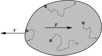
Figure 1: Schematic of the interior model. Adatoms detach from the inner boundary of the vacancy island and diffuse subject to the electromigration force $F$ directed to the right. As a consequence, the entire island drifts to the left at speed $V$.

In the present paper we focus on the “interior model” introduced by PLE. Referring to Fig. 1, we consider a single vacancy island which is isolated from the surrounding upper terrace by a strong step edge barrier that prevents adatoms from entering across the descending step ($k_{-}=0,\;d_{-}=\infty$). Diffusive motion of vacancy islands mediated by internal terrace diffusion has been observed experimentally on the Ag(110) surface Morgenstern et al. (2001). The mathematically equivalent process of internal diffusion of vacancies also plays an important role in the motion of adatom islands Heinonen et al. (1999). We will use the terminology appropriate for adatom diffusion inside a vacancy island throughout the paper.

The mathematical description of the interior model leads to a moving boundary value problem on a finite domain, which we formulate in the next section. A key ingredient of our analytic work is a separation ansatz for the adatom concentration, which allows us to determine stationary island shapes and investigate their linear stability in a simpler and more transparent way than in previous work Pierre-Louis and Einstein (2000). The analytic approach is complemented by numerical simulations of the full nonlinear and nonlocal dynamics. Specifically, in Section III we compute non-circular stationary island shapes perturbatively in the parameter $\delta=d_{+}/R_{0}$, where $R_{0}$ is the radius of the circle which solves the stationary problem in the TD limit ($d_{+}=0$). Section IV is devoted to the linear stability analysis of the circular solution for $d_{+}=0$. In agreement with PLE, we find that the eigenvalues of the linearized problem depend only on the ratio $z=R_{0}/\xi$, where

$$\xi=\frac{k_{\mathrm{B}}T}{F}$$ (2)

is the characteristic length scale associated with the electromigration force $F$. However, in contrast to PLE, who argued (on the basis of a less extensive analysis) that the circle becomes unstable for $z>0.1$, we show that it in fact remains linearly stable for all values of $z$. Simulations of the full nonlinear evolution in Section V nevertheless reveal an instability under finite amplitude perturbations, in which a finger develops at the trailing end of the island and eventually leads to a pinch-off. In Section VI we summarize our results and discuss their significance in the broader context of morphological stability in moving boundary value problems.

II Model

Since we assume that the mass transport on the surface is dominated by terrace diffusion, the main dynamical quantity of interest is the adatom concentration $c(x,y,t)$ on the terrace. By mass conservation its time evolution is governed by

$$\partial_{t}c+\nabla\cdot\vec{j}=0$$ (3)

$$\vec{j}=-D\nabla c+\frac{D}{\xi}\hat{x}c,$$ (4)

where the current $\vec{j}$ takes into account the contributions from diffusion and electromigration. Since we assume the force to be constant, electromigration appears as a drift in the direction of the electric current, denoted by the unit vector $\hat{x}$.

The coupling to the periphery of the island is given by the boundary conditions at the step edge. Let the subscripts $+,\,-$ denote quantities at the lower and upper terrace, respectively, $\vec{n}$ the normal pointing from the upper to the lower terrace, and $v$ the normal velocity of the island boundary. The fluxes

$$j_{\pm}:=\mp(\vec{j_{\pm}}\cdot\vec{n}-c_{\pm}v)$$ (5)

from the lower ($+$) and the upper ($-$) terrace, respectively, towards the step are then assumed to be proportional to the deviation from equilibrium Krug (2005), i.e.,

$$j_{\pm}=k_{\pm}(c_{\pm}-c_{\mathrm{eq}}),$$ (6)

with $k_{+},\,k_{-}$ denoting the attachment rates from the lower and upper terrace, respectively. Here the equilibrium density $c_{\mathrm{eq}}$ is given by the linearized Gibbs-Thomson relation

$$c_{\mathrm{eq}}=c^{0}_{\mathrm{eq}}(1+\Gamma\kappa),\qquad\Gamma=a^{2}\tilde{\gamma}/k_{\mathrm{B}}T,$$ (7)

where $\tilde{\gamma}$ denotes the (isotropic) step stiffness, $a$ the lattice constant, and $\kappa$ the curvature of the terrace boundary. The validity of (7) requires the capillary length $\Gamma$ to be small compared to the radius of curvature of the island boundary. Defining the kinetic lengths by (1), we note that in the terrace diffusion limit (TD), where the attachment/detachment becomes instantaneous ($k_{\pm}\to\infty$, $d_{\pm}\to 0$), the boundary conditions (6) reduce to

$$c=c_{\mathrm{eq}}.$$ (8)

Finally, by mass conservation, the normal velocity $v$ of the boundary is

$$v=a^{2}(j_{+}+j_{-}).$$ (9)

We neglect periphery diffusion, since we are concerned here with the kinetic regime where terrace diffusion is the dominant mass transport mechanism. For the interior model $k_{-}=0$, which implies $j_{-}=0$, and (8) applies on the interior (lower) terrace in the TD limit.

In the following, it is assumed that the electric current is in the $x$-direction, i.e. $\hat{x}=(1,0)$. Moreover, for analytic calculations the quasistatic approximation is frequently used, which amounts to setting $\partial_{t}c=0$ in the diffusion equation (3), which then reduces to

$$\Delta c-\xi^{-1}\partial_{x}c=0$$ (10)

and omitting the term proportional to $v$ in (5), which arises from the sweeping of adatoms by the moving step. For our purposes, the general solution of (10) is most conveniently expressed in polar coordinates. To arrive at a suitable representation, we first eliminate the drift term breaking the rotational symmetry of (10) via the ansatz

$$c(x,y)=\exp(\frac{x}{2\xi})f(\frac{x}{2\xi},\frac{y}{2\xi}),$$

which leads to the Helmholtz equation $\Delta f=f$. Separation of the latter equation yields a harmonic angular dependence and a modified Bessel function of imaginary argument $I_{n}$ for the radial part. The general solution of (10) is then a superposition of the form

$$c(r,\theta) =\exp(\tfrac{r}{2\xi}\cos\theta)f(r,\theta),$$ (11)

$$f(r,\theta) =\sum_{n=-\infty}^{\infty}\hat{c}_{n}I_{n}(\tfrac{r}{2\xi})\exp(in\theta),$$ (12)

where the unknown coefficients $\{\hat{c}_{n}\}$ are to be determined by the boundary conditions (6).

We further note that, in the quasistatic approximation, the total area $A$ of the island is strictly conserved by the dynamics. For the interior model one computes

$$\frac{d}{dt}A=\int_{\partial\Omega}v\;ds =-a^{2}\int_{\partial\Omega}\vec{j}_{+}\cdot\vec{n}\;ds$$

$$=-a^{2}\int_{\Omega}\nabla\cdot\vec{j}_{+}\;dA=0,$$

using the divergence theorem, where $\Omega$ denotes the interior domain and $\partial\Omega$ its boundary. The last integral vanishes in the quasistatic approximation. This means that the mass exchange between the island boundary (the bulk) and the adatom concentration inside is always balanced. In this sense the diffusion field merely mediates the mass transport from one part of the boundary to another.

III Steady states

For the interior model in the TD limit ($d_{+}=0,\;d_{-}=\infty$), circular islands are steady states. More precisely, an island with radius $R_{0}$, constant adatom concentration

$$c=c_{0}=c^{0}_{\mathrm{eq}}(1-\tfrac{\Gamma}{R_{0}})$$

and drifting with constant velocity

$$\vec{V}=-\frac{D}{\xi}\frac{a^{2}c_{0}}{1-a^{2}c_{0}}\hat{x}$$ (13)

is a solution of (3)-(9); the factor $(1-a^{2}c_{0})^{-1}$ is a correction to the quasistatic approximation, which requires $a^{2}c_{0}\ll 1$. However, if the attachment is not instantaneous ($d_{+}>0$), the circle is no longer stationary. As was shown in Pierre-Louis and Einstein (2000), an expansion of the interior model to second order in $z=R_{0}/\xi$ leads to noncircular steady states being elongated perpendicular to the field direction.

In the following we will investigate the existence of steady states in the regime where $z\sim 1$. To this end, we expand the interior model in the small parameter

$$\delta=d_{+}/R_{0}$$

and look for first order perturbations of the steady state, i.e.

$$R(\theta) =R_{0}+\rho(\theta)+{\mathcal{O}}(\delta^{2}),$$

$$\qquad c(r,\theta) =c_{0}+c_{1}+{\mathcal{O}}(\delta^{2}).$$

Applying the quasistatic approximation, this leads to the following linear system for $c_{1}$ and $\rho$:

$$\Delta c_{1}-\xi^{-1}\partial_{x}c_{1} =0,$$ (14)

$$c_{1}-d_{+}\xi^{-1}c_{0}\cos\theta =c^{0}_{\mathrm{eq}}\frac{\Gamma}{R_{0}^{2}}(\rho+\rho^{\prime\prime}),$$ (15)

$$0=\partial_{t}\rho =-(v_{1}-\vec{V}\cdot\vec{n})$$

$$=a^{2}D\big{(}\frac{c_{1}}{\xi}\hat{x}\cdot\vec{n}_{0}-\nabla c_{1}\cdot\vec{n}_{0}\big{)},$$ (16)

where $\vec{n}_{0}=(-\cos\theta,\sin\theta)$ is the normal of the circular steady state.

With the ansatz (11) for $c_{1}$, the steady state condition (16) is equivalent to

$$0 =\partial_{r}f-\tfrac{1}{2\xi}f\cos\theta.$$

Next, using (12) and property (27) of the Bessel functions $I_{n}$ leads to the following simple recursion relation for the coefficients $\hat{c}_{n}$:

$$\hat{c}_{n-1}I_{n-1}+\hat{c}_{n+1}I_{n+1}=\hat{c}_{n}\big{(}I_{n-1}+I_{n+1}\big{)},$$ (17)

where we have used the notation $I_{m}=I_{m}(R_{0}/2\xi)$. For a solution that is symmetric under reflection at the $x$-axis (field direction) we have $\hat{c}_{n}=\hat{c}_{-n}$, which together with (17) implies that $\hat{c}_{n}\equiv\hat{c}_{0}$. Therefore any symmetric solution of (14),(16) is of the form

$$c_{1}(r,\theta) =\hat{c}_{0}\exp(\tfrac{r}{2\xi}\cos\theta)\sum_{n=-\infty}^{\infty}I_{n}(\tfrac{r}{2\xi})\exp(in\theta)$$

$$=\hat{c}_{0}\exp(\tfrac{r}{\xi}\cos\theta),$$

where in the second identity we have used (29). Now the boundary condition (15) is used to fix the constant $\hat{c}_{0}$ as follows: First note that (15) describes a driven harmonic oscillator in ”time” $\theta$, with the left hand side being the driving force. Next recall that a $2\pi$ periodic solution $\rho(\theta)$ of this oscillator exists provided the driving force is $2\pi$-periodic with vanishing $n=1$ Fourier mode, where the latter condition means that the oscillator is not in resonance with the driving force. Using the Fourier expansion of $c_{1}$ (see (29)) this determines the constant $\hat{c}_{0}$ to be

$$\hat{c}_{0}=d_{+}\frac{c^{0}_{\mathrm{eq}}(1-\tfrac{\Gamma}{R_{0}})}{2\xi I_{1}(z)},\quad z=\frac{R_{0}}{\xi}.$$

Thus, the steady state adatom concentration is given by

$$c_{1}(r,\theta)=d_{+}\frac{c^{0}_{\mathrm{eq}}(1-\tfrac{\Gamma}{R_{0}})}{2\xi I_{1}(z)}\exp(\tfrac{r}{\xi}\cos\theta).$$

Finally, the symmetric steady state shape ($\rho(\theta)=\rho(-\theta)$) is obtained as the solution of the ordinary differential equation (15) as:

$$\rho(\theta)=\rho_{0}(z)+\sum_{n\geq 2}\rho_{n}(z)\cos n\theta$$

$$=R_{0}\delta z\frac{(\tfrac{R_{0}}{\Gamma}-1)}{I_{1}(z)}\Big{(}\tfrac{1}{2}I_{0}(z)+\sum_{n\geq 2}^{\infty}\frac{I_{n}(z)}{1-n^{2}}\cos n\theta\Big{)}.$$ (18)

The relative perturbation $\rho/R_{0}$ is expressed as a function of the dimensionless parameters $\delta=d_{+}/R_{0}$, $z=R_{0}/\xi$ and $\Gamma/R_{0}$, which characterize the deviation from the TD limit, the strength of the electromigration force and the capillary effects, respectively.

Figure 2: First order perturbations of the circular steady state. Left: Steady state shape for different values of $\delta=d_{+}/R_{0}\ll 1$ with fixed $z=R_{0}/\xi=5$ and $\Gamma/R_{0}=0.05$. Right: Different values of $z$ with fixed $\delta z=0.05$. In both cases the perturbed shape $R_{0}+\rho-\rho_{0}$ is depicted, i.e. the dilation mode has been subtracted.

The constant term $\rho_{0}$ in (18) describes a uniform dilation of the circle. Since $\Gamma/R_{0}\ll 1$, $\rho_{0}>0$, while $\rho_{n\geq 2}<0$. In particular, the leading order deformation with $n=2$ corresponds to an elongation perpendicular to the drift direction. This is illustrated in Fig. 2, where the dilation mode has been subtracted. Moreover, with increasing electromigration force (increasing $z$), the shapes start to become concave on the trailing side (recall that the islands are moving to the left).

As has been pointed out above in Section II, the full (nonlinear) evolution is area conserving in the quasistatic limit. Since the dilation mode $\rho_{0}$ is of the same order as the elongation mode $\rho_{2}$, this property is generally violated by the first order perturbation in $\delta$. This suggests that the perturbative regime may be restricted to rather small elongations. To obtain the steady states of the full nonlinear model, numerical simulations of the time-dependent equations (3)-(9) have been performed. An adaptive finite element method is used, where the free boundary problem is discretized semi-implicitly using an operator splitting approach and two independent numerical grids for the adatom density $c$ and for the island boundary, respectively. For the boundary evolution, a front tracking method is applied, for details see Bänsch et al. (2004).

Starting with a circular shape, the void elongates until it reaches a steady state. A typical example of the time evolution is depicted in Fig. 3.

Figure 3: Simulation of the full nonlinear evolution of a circular vacancy island towards a steady state. For this example, $\delta=0.1$ and $z=5$, which is well beyond the regime of validity of the first order perturbation theory. The void is moving from right to left and the snapshots are taken at $t=0$, $t=1.5$, $t=5$, $t=50$. The contours at later times are moved back to the right for better visibility. Space is measured in units of the radius $R_{0}$ of the initial shape and time in units $t_{0}=R_{0}/|\vec{V}|$, where $\vec{V}$ is the drift velocity of a circular island as given in (13). The simulation parameters are $R_{0}=100a,\;a^{2}c^{0}_{\mathrm{eq}}=10^{-5},\;\Gamma/R_{0}=0.05$.

Here the parameters are $\delta=0.1$, $z=5$, which, as will be seen below, is already far away from the perturbative regime. We do not observe any concave parts at the back side of the void as opposed to the perturbative steady state, see Fig. 2. This turns out to be true for all examples which we investigated. We also checked that the final steady state does not depend on the initial shape. For example, starting with a ”bean-like” shape being the steady state shape as obtained from the perturbation theory also leads to the same convex steady state. Moreover, we have not seen any break up in the simulations even for cases where $\delta\sim 1$. In all cases, a steady state shape similar to the one depicted in Fig. 3 is approached, where the deformation increases with increasing $\delta$ and where the curvature at the back side (right side) approaches zero. In Fig. 4 the steady states as obtained from the nonlinear evolution are depicted for different values of $\delta$.

Figure 4: Steady state shape as approached by the nonlinear evolution for different values of $\delta=d_{+}/R_{0}\ll 1$ with fixed $z=R_{0}/\xi=5$ and $\Gamma/R_{0}=0.05$.

By comparing with Fig. 2 (left) it is clear that the perturbative regime is limited to rather small values of $\delta$, since already for $\delta=0.01$ the perturbative (non-convex) and the nonlinear (convex) steady state shapes differ considerably.

In Fig. 5 we have investigated this quantitatively by comparing the deformation $\Delta$

$$\Delta=\big{(}\rho(\pi/2)+\rho(-\pi/2)-\rho(0)-\rho(\pi)\big{)}/2R_{0}$$

for the steady state obtained by the perturbation theory, i.e. given in (18), and for the steady state as approached by simulations of the full nonlinear dynamics. The first order perturbation theory is seen to be quantitatively accurate only for $\delta<0.01$.

Figure 5: Deformation $\Delta$ of the steady state shape versus relative kinetic length $\delta=d_{+}/R_{0}$, as obtained from perturbation theory and from the full model.

IV Linear stability analysis

Next we perform a linear stability analysis for the circular steady state of the interior model in the TD limit. Thus we are looking for small perturbations of the form

$$\rho(\theta,t) =\rho(\theta,0)\exp(i\omega t),$$

$$c_{1}(r,\theta,t) =c_{1}(r,\theta,0)\exp(i\omega t).$$

As in (14)-(16) we obtain – using the quasi-static approximation for $c_{1}$ – the following linearized system for $c_{1}$ and $\rho$,

$$\Delta c_{1} -\xi^{-1}\partial_{x}c_{1}=0,$$ (19)

$$c_{1} =c^{0}_{\mathrm{eq}}\frac{\Gamma}{R_{0}^{2}}(\rho+\rho^{\prime\prime}),$$ (20)

$$\partial_{t}\rho =a^{2}D\big{(}\frac{c_{1}}{\xi}\hat{x}\cdot\vec{n}_{0}-\nabla c_{1}\cdot\vec{n}_{0}\big{)}.$$ (21)

In view of (11) we make the following ansatz

$$\rho(\theta,0) =\exp(\tfrac{z}{2}\cos\theta)\sum_{n}\rho_{n}\exp(in\theta),\quad z=\frac{R_{0}}{\xi}.$$ (22)

Thus, the perturbation $\rho(\theta,0)$ is written as a series expansion in the functions $\exp(\tfrac{z}{2}\cos\theta)\exp(in\theta)$, instead of the usual Fourier modes. This choice has the advantage of simplifying the subsequent calculation. In particular it will lead to a linear system, where each matrix row/column has only a small number of non zero entries. However, as we will discuss later, the non-orthogonality of the ansatz functions increases the non-normality of the matrix. Equation (21) now takes the form

$$i\omega\sum\rho_{n}\exp(in\theta)=a^{2}D\big{(}\partial_{r}f-\tfrac{1}{2\xi}f\cos\theta\big{)}.$$

Using (12), (27) and matching coefficients we obtain

$$i\omega\rho_{n}= \frac{a^{2}D}{4\xi}\Big{(}\hat{c}_{n}\big{(}I_{n-1}+I_{n+1}\big{)}$$

$$\qquad-\hat{c}_{n-1}I_{n-1}-\hat{c}_{n+1}I_{n+1}\Big{)},$$ (23)

where here and in the following we use the notation $I_{n}=I_{n}(\tfrac{z}{2})$. We will finally use the linearized boundary condition (20) to express the coefficients $\hat{c}_{n}$ in (23) in terms of the $\rho_{n}$’s. Inserting the ansatz (11) for $c_{1}$, and (22) for $\rho$ into (20) yields

$$f(R_{0},\theta) =c^{0}_{\mathrm{eq}}\frac{\Gamma}{R_{0}^{2}}\sum\Big{(}1+\frac{z^{2}}{8}(1-\cos 2\theta)-\frac{z}{2}\cos\theta$$

$$\qquad-inz\sin\theta-n^{2}\Big{)}\rho_{n}\exp(in\theta),$$

which leads to (using (12) for the left hand side)

$$\hat{c}_{n}I_{n}(\tfrac{z}{2}) =c^{0}_{\mathrm{eq}}\frac{\Gamma}{R_{0}^{2}}\Big{(}\big{(}1+\frac{z^{2}}{8}-n^{2}\big{)}\rho_{n}-\frac{z^{2}}{16}\big{(}\rho_{n+2}+\rho_{n-2}\big{)}$$

$$\qquad-\frac{z}{4}\big{(}(2n-1)\rho_{n-1}-(2n+1)\rho_{n+1}\big{)}\Big{)}.$$ (24)

Inserting (24) into (23) leads after some tedious but straight forward calculations to the following eigenvalue problem for the coefficients $\{\rho_{n}\}$ and $\omega$:

$$\lambda\rho_{n} =\Big{(}\frac{z}{2}\big{(}1+\frac{z^{2}}{8}-n^{2}\big{)}C_{n}+\frac{z^{2}}{8}\Big{)}\rho_{n}$$

$$+\Big{(}\frac{z}{4}n(n+2)+(2n+1)\frac{z^{2}}{8}C_{n}-\frac{z^{3}}{64}\Big{)}\rho_{n+1}$$

$$+\Big{(}\frac{z}{4}n(n-2)+(-2n+1)\frac{z^{2}}{8}C_{n}-\frac{z^{3}}{64}\Big{)}\rho_{n-1}$$

$$-\Big{(}\frac{z^{2}}{16}(2n+3)+\frac{z^{3}}{32}C_{n}\Big{)}\rho_{n+2}$$ (25)

$$+\Big{(}\frac{z^{2}}{16}(2n-3)-\frac{z^{3}}{32}C_{n}\Big{)}\rho_{n-2}$$

$$+\frac{z^{3}}{64}\big{(}\rho_{n+3}+\rho_{n-3}\big{)},$$

with

$$\lambda=\frac{i\omega R_{0}^{3}}{a^{2}c^{0}_{\mathrm{eq}}D\Gamma},\;\;\;C_{n}=\frac{I_{n+1}+I_{n-1}}{2I_{n}}=\frac{I_{n+1}}{I_{n}}+\frac{2n}{z}.$$

The right hand side of (IV) represents the linearized time evolution of the island as a (infinite) matrix $\hat{A}$ acting on the coefficients $\rho_{n}$. In real space it corresponds to an integro-differential operator, which is essentially nonlocal. Remarkably, the matrix depends on the system parameters only through the dimensionless electromigration force $z=R_{0}/\xi$. In particular, the capillary length $\Gamma$ affects the time scale of the linear evolution, but not the stability of specific perturbations Pierre-Louis and Einstein (2000). For $\Gamma\to 0$, all eigenfrequencies $\omega_{n}$ vanish, which implies that all perturbations become marginal. Indeed, it is easy to check that in the TD limit, for $\Gamma=0$, any island shape translates rigidly at constant velocity under (3)–(9).

The matrix $\hat{A}$ exhibits a symmetry, which originates from the invariance of the system under reflection at the $x$-axis (field direction). In terms of the coefficients $\rho_{n}$ this reflection is expressed as $\rho_{n}\to\rho_{-n}$, and one readily verifies that this does leave (IV) unchanged. Accordingly the eigenspace splits into two invariant subspaces with symmetric and antisymmetric eigenmodes characterized by

$$\rho_{n} =\rho_{-n} \mathrm{symmetric}$$

$$\rho_{n} =-\rho_{-n} \mathrm{antisymmetric}.$$

In both cases the eigenmodes are fully determined by only half of the coefficients (e.g. those with positive index), which allows us to reduce (IV) to a semi-infinite system. By truncating it towards large $n$ (cutoff towards small wavelengths) we arrive at a finite linear system which we solve numerically.

Before we present the numerical results, we discuss translations and dilations, which are perturbations related to the symmetry properties of the system. Symmetry under translations in the horizontal ($x$) and vertical ($y$) direction leads to two zero eigenmodes $\mathcal{T}_{x}$, $\mathcal{T}_{y}$ – the infinitesimal horizontal and vertical translations – given by

$$\mathcal{T}_{x}(\theta)=\cos(\theta),\quad\mathcal{T}_{y}(\theta)=\sin(\theta).$$

Indeed, inserting $\rho=\mathcal{T}_{x}$ or $\rho=\mathcal{T}_{y}$ into the linearized boundary condition (20) leads to $c_{1}\equiv 0$ and therefore (21) yields $\partial_{t}\rho\equiv 0$. The horizontal translation $\mathcal{T}_{x}$ belongs to the symmetric eigenmodes, while the vertical translation $\mathcal{T}_{y}$ belongs to the antisymmetric class. Next we consider a dilation $\mathcal{D}$, i.e., a constant initial perturbation

$$\mathcal{D}(\theta)=1.$$

Inserting $\rho(\theta)=\mathcal{D}(\theta)=1$ into the boundary condition (20) yields

$$c_{1}=\frac{c_{\mathrm{eq}}^{0}\Gamma}{R_{0}^{2}},$$

which reflects the fact that one passes from one stationary solution to another by increasing the radius of the island and the concentration inside the island by a constant value. However, a dilation is not a zero eigenmode: Since we consider perturbations of a circular steady state, which has a steady state drift velocity depending on the radius, two circles with different radius are drifting apart. This leads to a linear increase of the perturbation. From (21), an initial perturbation $\rho(\theta,0)=1$ has to grow according to

$$\partial_{t}\rho=\frac{a^{2}c_{\mathrm{eq}}^{0}\Gamma D}{R_{0}^{2}\xi}\cos(\theta)=\frac{a^{2}c_{\mathrm{eq}}^{0}\Gamma D}{R_{0}^{2}\xi}\mathcal{T}_{x}(\theta).$$

In that sense a dilation $\mathcal{D}$ generates a translation, and $\mathcal{D}$ is a generalized eigenmode with eigenvalue zero according to $\hat{A}^{2}\mathcal{D}\sim\hat{A}\mathcal{T}_{x}=0$. Thus (restricting to the symmetric case) the eigenvalue zero is two-fold degenerate, and has one (proper) eigenvector. Therefore the matrix $\hat{A}$ can not be diagonalized completely but contains a $2\times 2$ Jordan block corresponding to the invariant subspace spanned by $\mathcal{D}$ and $\mathcal{T}_{x}$. Apart from that, the dilation doesn’t play a role, because the time evolution preserves the area and we can therefore always restrict ourselves to perturbations which do not contain dilations.

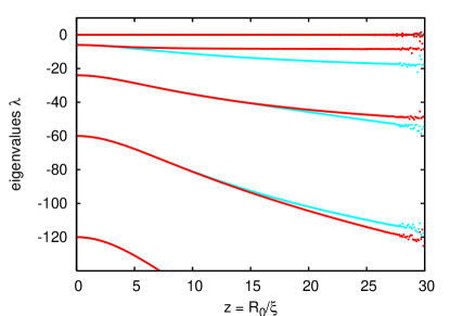
Figure 6: (Color online) Spectrum of the linearized theory as obtained by numerical solution of the eigenvalue problem (IV). Depicted are the eleven largest eigenvalues as a function of the dimensionless electromigration force $z=R_{0}/\xi$. Eigenvalues of symmetric modes are red/black, eigenvalues of antisymmetric modes blue/grey. Note that the eigenvalue zero is threefold degenerate. All negative eigenvalues come in pairs, consisting of a symmetric and an antisymmetric mode which become degenerate at $z=0$. For the fluctuations appearing around $z=30$ see the discussion at the end of Section IV.

The numerically determined spectrum is presented in Fig. 6. Here the largest eigenvalues, for $0\leq z\leq 30$ are depicted. The spectrum is purely real and apart from the predicted threefold degenerate zero eigenvalue it is strictly negative. For $z=0$ (no electromigration force), the right hand side of (IV) becomes diagonal:

$$\lambda\rho_{n}=|n|(n^{2}-1)\rho_{n},$$

which allows to directly read off the eigenvalues $\lambda_{n}=|n|(n^{2}-1)$. Each eigenvalue $\lambda_{n}$ is twofold degenerate with eigenmodes given by the Fourier modes $\cos(n\theta)$, $\sin(n\theta)$. Since no field breaks the rotational symmetry, the symmetric and antisymmetric modes $\cos(n\theta)$, $\sin(n\theta)$ are connected by a rotation by $\pi/2$ and belong to the same eigenvalue $\lambda_{n}$. In the presence of an electric current, i.e. $z>0$, the rotational symmetry is broken and the degeneracy is removed, i.e., the eigenvalues split. Moreover increasing values of $z$ lead to decreasing eigenvalues, i.e. larger islands or islands in the presence of a stronger field relax faster to the circular shape (as compared to the case without drift). For large values of $z$ the eigenvalue problem becomes numerically difficult to solve, leading to a noisy spectrum in Fig. 6 for values of $z\sim 30$. This will be discussed in more detail below.

We now turn to the eigenmodes of the linearized time evolution. Figs. 7 and 8 show some examples of symmetric and antisymmetric eigenmodes with small index $n$ for $z=10$. All of them reveal a typical undulated shape, where the number of nodes increases with the index and the amplitude is largest towards $\theta=0$. Thus the modulation is more pronounced at the back side of the island (with respect to the drift motion) and, as shown in Fig. 9, this localization gets stronger with increasing $z$. This is a signature of the fact that the eigenvectors become more and more parallel (see below). The increasing localization of the eigenmodes at the back side of the island may be traced back to the convective, electromigration-induced flux in the adatom diffusion equation (3) which leads to the factor $\exp(\tfrac{z}{2}\cos\theta)$ in (22). For large values of $z$, this factor strongly suppresses all contributions for values of $\theta$, which are not close to $\theta=0$. In particular, a perturbation that is front-back symmetric has to be a linear combination of many different eigenmodes. In that case, the eigenmodes with large index $n$ will decay very fast leading to a shape being close to the steady state circular shape at the front side, while still having a large buckle at the back side.

This behaviour will be investigated in more detail in the next section, when we consider the fully nonlinear evolution. For large values of $z$ this will finally lead to a fingering instability at the back side of the island.

Figure 7: Second, fourth and sixth symmetric eigenmode as function of the angle $\theta$ ($z=10$). $\theta=\pi$ is the drift direction. The modes are normalized with respect to the $L^{2}$-norm.

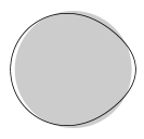
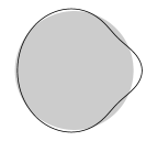
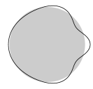
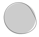
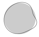
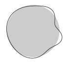
Figure 8: Second, third and fourth eigenmode superimposed on a circle (grey background) for $z=10$. Top (bottom) row shows symmetric (antisymmetric) modes.

Figure 9: Symmetric eigenmode $n=3$ for different values of $z$. The asymmetry with respect to front ($\theta=\pi$) and back side ($\theta=0$) increases with increasing value of $z$. The modes are normalized with respect to the $L^{2}$-norm.

Before turning to the nonlinear evolution, we comment on some observations connected with non-normal eigenvalue problems. The matrix $\hat{A}$ in (IV) is highly non-normal for large values of $z$, which leads to a strong sensitivity of the spectrum with respect to small perturbations of the matrix entries. Small changes of the entries of the matrix may lead to structurally completely different spectra, a feature which can be consistently described within the theory of pseudospectra Trefethen and Embree (2005). The degree of non-normality depends on the choice of the basis. In our case the basis is not orthogonal (with respect to the usual $L^{2}$ scalar product) and therefore, although convenient for the analytical part, can give a distorted picture of the underlying geometry. We therefore checked the results by transforming the system (IV) to the Fourier basis. Here the non-normality is much less pronounced and we obtained the same spectrum as depicted in Fig. 6. In both cases, we have not been able to obtain the spectrum numerically for values $z>30$ since, as can be seen from Fig. 6 the lines start to become noisy between $z=25$ and $30$. The fluctuations are getting stronger very quickly, making it impossible to determine the spectrum reliably.

A closer examination reveals that the condition numbers for the eigenvalues grow exponentially with $z$ and therefore the accuracy of the results gets lost very quickly at some point. This is again a consequence of the non-normality of the problem. The condition number of a given eigenvalue is large when the corresponding left and right eigenvectors are almost orthogonal Quarteroni et al. (2000). This is intimately connected with the non-orthogonality between different (right) eigenvectors. In our case the eigenvectors become almost parallel for large values of $z$. Even a slight perturbation of the matrix entries will destroy this and improve the condition numbers dramatically, of course by changing the spectrum beyond recognition.

Finally we note that non-normality has also been discussed Schimschak and Krug (1998); Trefethen et al. (1993); Grossmann (2000); Trefethen and Embree (2005) as a mechanism causing a transient growth of small perturbations even in the case of a linearly stable system. This transient amplification can be large enough to drive the system out of the linear regime, this way leading to an instability. We thoroughly investigated the transient behaviour of the linearized system and found that this scenario does not apply to our case.

V Nonlinear evolution

To further investigate the nonlinear evolution, we have performed numerical simulations of (3)-(9) using an adaptive finite element method, as described in Section III. We note that adaptive mesh refinement during the time evolution in regions with high curvature turned out to be crucial for accurate simulations in the case when small fingers appear in the shape.

We probe the nonlinear dynamics with a very strong electromigration force, i.e. choosing $z=R_{0}/\xi=25$. In Fig. 10 a simulation of a vacancy island (interior model) in the TD regime is depicted. Here an ellipse with aspect ratio $1.2$ has been taken as the initial shape.

Figure 10: Nonlinear dynamics in the interior model with strong electromigration force ($z=25$). The initial shape is an ellipse with aspect ratio $1.2$. A fingering instability appears at the trailing end, which leads to a pinch-off. The contours are shifted upwards for better visibility and also shifted to the right with $\Delta x=t|\vec{V}|$, where $\vec{V}$ is the drift velocity of a circular island, see (13). Space is measured in units of the lattice spacing $a$ and time in units $t_{0}=R_{0}/|\vec{V}|$. The simulation parameters are $R_{0}=100a,\;a^{2}c^{0}_{\mathrm{eq}}=10^{-5},\;\Gamma/R_{0}=0.02$. The breaking of the up-down symmetry in the right column is due to numerical noise.

We observe a fingering instability at the back side of the vacancy island, which finally leads to a pinch-off. Note that this behaviour has not been predicted by the linear stability theory.

To gain a better understanding of the nonlinear dynamics, the initial evolution of an ellipsoidal island has been investigated in more detail. For this special geometry, one may use elliptic coordinates and an expansion of the adatom concentration in terms of Mathieu functions to arrive at an analytic expression for the normal velocity, see Appendix B, (31). However, as it turned out, a reliable evaluation of the series expansion is possible only for moderate values of $z\leq 5$ and aspect ratios $\leq 2$. For parameters in this regime, the normal velocity of an ellipsoidal vacancy island – elongated in the horizontal direction – in the center of mass system, i.e. after subtracting the (fairly large) drift velocity, is compared with the corresponding results of the finite element simulation in Fig. 11.

Figure 11: Normal velocity of an ellipsoidal vacancy island (elongated in the horizontal direction) as a function of the normal angle in the center of mass system, i.e., after subtracting the drift velocity of the island. The normal points inwards, i.e. a positive velocity corresponds to local shrinking, and the angle $\theta=\pi$ corresponds to the drift direction. The normal velocity taken from the numerical simulations by averaging over the first $1000$ time steps is in very good agreement with the results obtained by evaluating the analytic solution using elliptic coordinates.

The two solutions are in very good agreement. Moreover, one realizes that the dynamics is fastest at the front part of the island and tends to relax the front half of the ellipse towards a circle, since the boundary moves inwards at $\theta=\pi$ ( front ) but outwards in nearby regions with $\theta\approx\pi\pm\pi/4$. Since the evolution at the back half of the island is slower and always inwards, we expect the dynamics to lead to an egg like shape, which is verified in the simulations, see Fig. 12. Moreover, the asymmetry of the dynamics becomes more pronounced with increasing values of $z$. We expect this to be a possible reason for the onset of a fingering instability, once a critical value of the curvature at the back end is reached.

Figure 12: Numerical simulation of the evolution of an ellipsoidal vacancy island with aspect ratio $2.0$ and area $\pi R_{0}^{2}$. The upper figure depicts the initial stage of the evolution: the left/right asymmetry increases with increasing value of $z=R_{0}/\xi$, leading to the formation of an egg-like shape. Bottom: For large values of $z$, the asymmetric evolution leads to a fingering instability at the back side of the island. Space is measured in units of the lattice spacing $a$ and time in units $t_{0}=R_{0}/|\vec{V}|$, where $\vec{V}$ is the drift velocity of a circular island as given in (13) for the case $z=10$. The simulation parameters are $R_{0}=100a,\;a^{2}c^{0}_{\mathrm{eq}}=10^{-5},\;\Gamma/R_{0}=0.05$.

To roughly locate the threshold for the onset of the instability we systematically varied the electromigration strength $z$ and the amplitude of the initial perturbation given as the aspect ratio of the initially horizontally elongated circle. The results of the simulations are presented in Fig. 13. As can be seen, the instability sets in around $z\sim 10$.

Figure 13: Threshold for the onset of the instability: Simulations for different values of $z=R_{0}/\xi$ and aspect ratios of the initial ellipsoid, where the elongation is in field direction, have been performed. The instability sets in at $z=9$. For $z\geq 11$ also the smallest aspect ratio leads to an instability, i.e. a fingering at the back side of the island.

Although we are so far lacking a satisfactory analytic understanding of the underlying mechanism, we would like to present some intuitive reasoning for the onset of an instability at large values of $z$. First recall that the mass flux at the boundary of the vacancy island in the normal direction $\vec{n}$ (pointing inwards) is the sum of the diffusive flux

$$j_{d}=-D\nabla c\cdot\vec{n}$$

and the flux caused by electromigration

$$j_{e}=\frac{D}{\xi}c_{\mathrm{eq}}\vec{n}\cdot\hat{x},$$

where, as usual, $\hat{x}$ denotes the unit vector in $x$-direction. Next we consider the two simplified cases of (a) $j_{e}=0$, i.e. no electric field and (b) $j_{d}=0$, i.e, no diffusion, to argue that $j_{d}$ is stabilizing while $j_{e}$ is destabilizing:

• No electric field: An outward bump of the boundary leads to a local maximum of the curvature and therefore a local minimum of the adatom density $c_{\mathrm{eq}}$ along the boundary. Due to the maximum principle, this will also be a local minimum of $c$ inside the island, leading to a diffusive flux towards the boundary, i.e., the bump will be filled. Thus the diffusive flux is stabilizing.

• No diffusion: Consider an outward bump of the boundary at the trailing (back) island edge. As in case (a), this leads to an increased curvature and therefore a decreased adatom density $c_{\mathrm{eq}}$ as compared to the front side. The flux $j_{e}$ caused by electromigration is proportional to $c_{\mathrm{eq}}$ and therefore decreased at the back side, i.e. this part of the boundary is now drifting more slowly than the center of mass and the bump is growing. Thus the electromigration flux destabilizes the trailing edge and stabilizes the leading edge of the island.

Finally consider the general case of an outward bump of the trailing boundary in the presence of diffusion and electromigration. Fixing all parameters, except the strength of the electric field, $\xi^{-1}$, the diffusive flux depends essentially on the geometry of the bump, whereas the decrease of $j_{e}$ is proportional to $\xi^{-1}$. Thus we may expect that the bump will grow if the electric field is large enough.

The argument also elucidates the role of the capillarity parameter $\Gamma$ in this problem, which is mainly to translate variations of the boundary curvature into variations of the adatom concentration in the interior of the island. The latter in turn underlies both the stabilizing effect of the diffusive current and the destabilizing effect of electromigration. In contrast to the instabilities in the PD regime, which can be described in terms of a competition between capillarity and electromigration Schimschak and Krug (1998); Kuhn and Krug (2005); Kuhn et al. (2005), here capillarity plays a largely neutral part, which explains (in hindsight) why the linear stability properties are independent of $\Gamma$ (see Section IV).

VI Conclusions

In this paper, we have presented a detailed study of a continuum model for the electromigration-driven shape evolution of single-layer vacancy islands mediated by internal terrace diffusion. Significant shape deformations, such as the elongation transverse to the field direction described in Section III or the pinch-off instability discussed in Sect.V, were found to require dimensionless electromigration forces $z=R_{0}/\xi$ significantly larger than unity. Unfortunately this implies that these phenomena will be difficult to realize experimentally, at least for the surfaces commonly used in this context. To give an example, the maximal electromigration bias that can be achieved on the Cu(100) surface has been estimated Mehl et al. (2000) to be on the order of $E_{\mathrm{bias}}\approx 10^{-5}$ eV for a diffusion hop between nearest neighbor sites, corresponding to a characteristic length scale $\xi/a=k_{\mathrm{B}}T/E_{\mathrm{bias}}\approx 2.5\times 10^{3}$. An island with $z=10$ would thus contain about $2\times 10^{9}$ atoms, which is four orders of magnitude larger than the size at which strong shape deformations and electromigration-induced oscillatory dynamics have been predicted in the PD regime Rusanen et al. (2006).

From the broader perspective of the theory of moving boundary value problems, our results are of interest because they add another example to the list of cases in which the standard tool of linear stability analysis fails to correctly predict the stability properties of the full nonlinear dynamics. The behavior of the interior model in the TD limit is similar in many respects to the void migration problem in the PD regime which was studied in Schimschak and Krug (1998, 2000). In both cases the circular solution is linearly stable for arbitrary values of the electromigration force, but a nonlinear instability occurs when the system is subjected to finite amplitude perturbations, and the threshold for the nonlinear instability decreases with increasing force. Moreover, as in the case of void migration, a distorted island either relaxes back to the circular shape or evolves towards pinch-off. This suggests (as has been proven for voids Cummings et al. (2001)) that no non-circular stationary states exist. However, in contrast to the void migration problem, in the present study we found no evidence for transient amplification of linear perturbations related to the non-normality of the eigenvalue problem.

In this context it is worth mentioning the problem of two-dimensional ionization fronts, which shares some of the features of both void and island migration Meulenbroek et al. (2005). In this system a closed curve representing the ionized region (a “streamer”) evolves in response to a Laplacian potential in the exterior domain. As in the void migration problem, a constant potential gradient far away from the streamer represents the driving electric field. However, the boundary condition at the front is similar to that employed in the present work, (5,6,9) with $c_{\mathrm{eq}}=\mathrm{const.}$, i.e. $\Gamma=0$, and the kinetic length corresponds to the width of the ionization front. Again, circles translating at constant velocity are solutions of the problem. In the special case where the kinetic length equals the radius of the streamer the linearized dynamics can be solved exactly, and it is found that the circle is always stable. Standard linear stability analysis nevertheless fails, because smooth initial perturbations do not decay exponentially Ebert et al. (2006). Further exploration of the relationship between these three boundary value problems seems like a promising direction for future research.

Appendix A Bessel functions

We summarize some properties of the modified Bessel functions of imaginary argument $I_{n}$. For integer $n$ the functions $I_{n}$ are symmetric with respect to the index

$$I_{-n}(r)=I_{n}(r).$$ (26)

The derivative is

$$\tfrac{d}{dr}I_{n}(r)=\tfrac{1}{2}(I_{n-1}(r)+I_{n+1}(r)).$$ (27)

There is the recursion relation

$$rI_{n-1}(r)-rI_{n+1}(r)=2nI_{n}(r),$$ (28)

and the generating function is

$$\exp(r\cos\theta)=\sum_{n=-\infty}^{\infty}I_{n}(r)\exp(in\theta).$$ (29)

Appendix B Normal velocity of an ellipsoidal island

To calculate the concentration profile inside an ellipsoidal island, we introduce elliptic coordinates

$$x=\alpha\cosh(u)\cos(w),$$

$$y=\alpha\sinh(u)\sin(w),$$

where $u$ and $w$ are the radial and angular coordinates, respectively. The line $u\equiv u_{0}=\mathrm{const.}$ is an ellipse with aspect ratio $\tanh(u_{0})$ and the parameter $\alpha$ determines the size of this ellipse. Curvature and normal vector are

$$\kappa =-\frac{1}{\alpha g^{\frac{3}{2}}}\cosh(u_{0})\sinh(u_{0}),$$

$$\vec{n} =\frac{1}{\sqrt{g}}\left(\begin{array}[]{c}\sinh(u_{0})\cos(w)\\ \cosh(u_{0})\sin(w)\end{array}\right),$$

with $g=\cosh^{2}(u_{0})-\cos^{2}(w)$. The Helmholtz equation now reads

$$(\partial_{u}^{2}+\partial_{w}^{2})f=\alpha^{2}(\sinh^{2}(u)+\sin^{2}(w))f$$

and separation $f(u,w)=f_{u}(u)f_{w}(w)$ leads to

$$f_{w}^{\prime\prime}-\alpha^{2}\sin^{2}(w)f_{w} =\lambda f_{w},$$

$$-f_{u}^{\prime\prime}+\alpha^{2}\sinh^{2}(u)f_{u} =\lambda f_{u}.$$

The solutions of the two equations are related by $f_{w}(ix)=f_{u}(x)$. Requiring periodicity of $f_{w}$ determines a discrete set of values for the separation parameter $\lambda$. The corresponding solutions are the Mathieu functions of the first kind $\mathrm{ce}_{n}$ and $\mathrm{se}_{n}$ Gradshteyn and Ryzhik (2000). Since the ellipse is symmetric with respect to the field direction we only need the $\mathrm{ce}_{n}$ which are even functions of the angular variable $w$. The general solution is then

$$c(u,w)=\exp\left(\frac{\alpha}{2\xi}\cosh(u)\cos(w)\right)\sum_{n=0}^{\infty}b_{n}\mathrm{ce}_{n}(w)\mathrm{ce}_{n}(iu).$$ (30)

The coefficients $b_{n}$ are determined by the boundary condition (8). The Mathieu functions are orthogonal and normalized according to $\int_{0}^{2\pi}\mathrm{ce}_{n}^{2}(x)\;dx=\pi$. Thus, the $b_{n}$ can be found in a way similar to Fourier coefficients via the integrals

$$b_{n} =\frac{c^{0}_{\mathrm{eq}}}{\pi\mathrm{ce}_{n}(iu_{0})}\int_{0}^{2\pi}\mathrm{ce}_{n}(w)\exp\left(-\frac{\alpha}{2\xi}\cosh(u_{0})\cos(w)\right)\times$$

$$\times(1-\Gamma\kappa)\;dw.$$

These integrals are solved numerically. Finally, using the general solution (30) to calculate the flux to the boundary, the normal velocity $v$ of the island edge is obtained as

$$v =\frac{a^{2}D}{\sqrt{g}}\exp\left(\frac{\alpha}{2\xi}\cosh(u_{0})\cos(w)\right)\sum b_{n}\mathrm{ce}_{n}(w)\times$$

$$\times\left(\frac{1}{\alpha}\mathrm{Im}(\mathrm{ce}_{n}^{\prime}(iu_{0}))+\frac{1}{\xi}\sinh(u_{0})\cos(w)\mathrm{ce}_{n}(iu_{0})\right).$$ (31)