Abstract

We study the vacuum state of spin chains where each site carry an arbitrary representation. We prove that the string hypothesis, usually used to solve the Bethe ansatz equations, is valid for representations characterized by rectangular Young tableaux. In these cases, we obtain the density of the center of the strings for the vacuum. We work out different examples and, in particular, the spin chains with periodic array of impurities.

MSC: 81R50, 17B37 — PACS: 02.20.Uw, 03.65.Fd, 75.10.Pq

LAPTH-1171/07

cond-mat/0701207

January 2007

1 Introduction

Since the seminal work of H. Bethe [1] solving the spin $\frac{1}{2}$ Heisenberg spin chain [2], numerous applications of this method have been appeared to solve more involved models: anisotropic XXZ spin chain [3, 4, 5]; spin 1 chains [6, 7]; alternating spin chains [8, 9, 10, 11]; spin chains with higher spins [12, 13, 14, 15, 5, 16, 17, 18, 19]; spin chains with boundaries [20, 21, 22, 23] or with impurities [24, 25, 26]. In the papers [15, 27], the Bethe ansatz equations (BAE) have been obtained for spin chains based on $gl(N)$ and where each site may carry a different representation. This generic framework encompasses the models with higher spin on each site or with impurities and the alternating spin chains.

In this paper, we are interested in the resolution of these equations within the thermodynamical limit, but keeping arbitrary the representation on each site. The first step consists in using the string hypothesis. We show that the consistency of the BAE implies a restriction on the representations involved in the spin chain. This restriction is solved by taking representations characterized by rectangular Young tableaux. For the other cases, the validity of the string hypothesis remains an open question. Then, we determine the vacuum state and prove that it is non degenerate and a trivial representation of the $sl(N)$ symmetry algebra. This vacuum state is constructed on strings whose lengths and multiplicities are explicitly given. Finally, the densities of the center of these strings are computed exactly. Throughout the paper, different examples are worked out. In particular, we treat in detail the spin chains with periodic array of impurities for which we compute the energy of the vacuum state.

The plan of this paper is as follows. In section 2, we recall basic notions and notations on Yangian algebras and spin chains. Section 3 is devoted to the study of the BAE within the string hypothesis, and the constraints it imposes on the representations entering the spin chain. The vacuum state is determined in section 4, see theorem 4.1. Section 5 is concerned with the resolution of the BAE within the thermodynamical limit. In particular, we compute the densities of the vacuum state, see theorem 5.2.

2 Generalities

2.1 Yangian ${\cal Y}(gl(N))$

We will consider the $gl(N)$ invariant $R$ matrices [28, 29]

$$R_{ab}(\lambda)={\mathbb{I}}_{N}\otimes{\mathbb{I}}_{N}+\frac{i\;{\cal P}_{ab}}{\lambda}\;,$$ (2.1)

where ${\cal P}_{ab}$ is the permutation operator

$${\cal P}_{ab}=\sum_{i,j=1}^{N}E_{ij}\otimes E_{ji}$$ (2.2)

and $E_{ij}$ are the elementary matrices with 1 in position $(i,j)$ and 0 elsewhere.

This $R$ matrix satisfies the Yang–Baxter equation [30, 28, 29, 4, 5]

$$R_{ab}(\lambda_{a}-\lambda_{b})\ R_{ac}(\lambda_{a})\ R_{bc}(\lambda_{b})=R_{bc}(\lambda_{b})\ R_{ac}(\lambda_{a})\ R_{ab}(\lambda_{a}-\lambda_{b})\;.$$ (2.3)

It can be interpreted physically as a scattering matrix [31, 4, 3] describing the interaction between two solitons (viewed in this framework as low level excited states in a thermodynamical limit of a spin chain) that carry the fundamental representation of $gl(N)$.

The Yangian ${\cal Y}(gl(N))$ [32] is the complex associative unital algebra with the generators $T_{ij}^{(n)}$ ($T_{ij}^{(0)}=\delta_{ij}$), for $1\leq i,j\leq N,n\in{\mathbb{Z}}_{\geq 0}$ subject to the defining relations, called FRT exchange relation [33],

$$R_{ab}(\lambda_{a}-\lambda_{b})\;{\cal T}_{a}(\lambda_{a})\;{\cal T}_{b}(\lambda_{b})={\cal T}_{b}(\lambda_{b})\;{\cal T}_{a}(\lambda_{a})\;R_{ab}(\lambda_{a}-\lambda_{b})\;,$$ (2.4)

where the generators are gathered in the following matrix (belonging to $End({\mathbb{C}}^{N})\otimes{\cal Y}(gl(N))[[\lambda^{-1}]]$)

$${\cal T}(\lambda)=\sum_{i,j=1}^{N}E_{ij}\otimes T_{ij}(\lambda)=\sum_{i,j=1}^{N}E_{ij}\otimes\sum_{r\geq 0}\frac{1}{\lambda^{r}}~{}T_{ij}^{(r)}=\sum_{r\geq 0}\frac{1}{\lambda^{r}}~{}{\cal T}^{(r)}\;.$$ (2.5)

Using the commutation relations (2.4), it is easy to show that ${\cal T}^{(1)}$ generates a $gl(N)$ algebra.

2.2 Algebraic transfer matrix

In the following, in order to construct spin chains, it will be necessary to deal with the tensor product of $L$ copies of the Yangian. For $1\leq i\leq L$, we denote by ${\cal L}_{ai}(\lambda)\in End({\mathbb{C}}^{N})\otimes{\cal Y}(gl(N))$ one copy of the Yangian which acts non trivially on the $i^{th}$ space only. The space $a$, always isomorphic to $End({\mathbb{C}}^{N})$ in the present paper, is called auxiliary space whereas the space $i$ is called quantum space. Mimicking the notation (2.5) used for ${\cal T}(\lambda)$, we will consider ${\cal L}_{ai}(\lambda)$ as an $N\times N$ matrix whose entries are operators acting on the quantum space $i$. These operators will be expanded as series in $\lambda$, so that we have

$${\cal L}_{ai}(\lambda)=\sum_{p,q=1}^{N}E_{pq}\otimes L_{pq}(\lambda)=\sum_{p,q=1}^{N}E_{pq}\otimes\sum_{r\geq 0}\frac{1}{\lambda^{r}}~{}L_{pq}^{(r)}=\sum_{r\geq 0}\frac{1}{\lambda^{r}}~{}{\cal L}_{ai}^{(r)}\;.$$ (2.6)

Obviously, ${\cal L}_{ai}(\lambda)$ satisfies the defining relations of the Yangian

$$R_{ab}(\lambda_{a}-\lambda_{b})\;{\cal L}_{ai}(\lambda_{a})\;{\cal L}_{bi}(\lambda_{b})={\cal L}_{bi}(\lambda_{b})\;{\cal L}_{ai}(\lambda_{a})\;R_{ab}(\lambda_{a}-\lambda_{b})\;.$$ (2.7)

Let us stress that the matrix ${\cal L}_{ai}(\lambda)$ is local, i.e. it contains only the $i^{th}$ copy of the Yangian. On the contrary, one constructs a non-local algebraic object, the monodromy matrix

$${\cal T}_{a}(\lambda) ={\cal L}_{a1}(\lambda)\;{\cal L}_{a2}(\lambda)\;\dots\;{\cal L}_{aL}(\lambda)\in End({\mathbb{C}}^{N})\otimes\left({\cal Y}(gl(N))\right)^{\otimes L}\;.$$ (2.8)

Let us remark that the quantum spaces are omitted in the LHS of (2.8), as usual in the notation of the monodromy matrix. The entries of the monodromy matrix ${\cal T}_{a}(\lambda)$ are given by

$$T_{ij}(\lambda) =\sum_{k_{1},\dots,\,k_{L-1}=1}^{N}L_{ik_{1}}(\lambda)\;\otimes\;L_{k_{1}k_{2}}(\lambda)\;\otimes\;\dots\;\otimes\;L_{k_{L-1}j}(\lambda)\;.$$ (2.9)

and satisfies the defining relations of the Yangian

$$R_{ab}(\lambda_{a}-\lambda_{b})\;{\cal T}_{a}(\lambda_{a})\;{\cal T}_{b}(\lambda_{b})={\cal T}_{b}(\lambda_{b})\;{\cal T}_{a}(\lambda_{a})\;R_{ab}(\lambda_{a}-\lambda_{b})\;.$$ (2.10)

Now, we can introduce the main object for the study of spin chains, i.e. the transfer matrix

$$t(\lambda)=tr_{a}\left({\cal T}_{a}(\lambda)\right)=\sum_{i=1}^{N}T_{ii}(\lambda)\;.$$ (2.11)

Equation (2.10) immediately implies

$$[\;t(\lambda)\;,\;t(\mu)\;]=0$$ (2.12)

which will guarantee the integrability of the models.

Let us remark that, at that point, the monodromy and transfer matrices are algebraic objects (in $\left({\cal Y}(gl(N))\right)^{\otimes L}$), and, as such, play the rôle of generating functions for the construction of monodromy and transfer matrices as they are usually introduced in spin chain models. The latter will be constructed from the former using representations of the Yangian, as it will be done below.

2.3 Representations

In order to construct representations of ${\cal Y}(gl(N))$, the following algebra homomorphism (called evaluation map, see e.g. [34]) from ${\cal Y}(gl(N))$ to ${\cal U}(gl(N))$ (universal enveloping algebra of $gl(N)$) will be used

$$L_{pq}(\lambda)\longmapsto\delta_{pq}+\frac{i\;e_{qp}}{\lambda}\;,$$ (2.13)

where $e_{pq}$ ($1\leq p,q\leq N$) are the abstract generators of the Lie algebra $gl(N)$. They satisfy the following commutation relations

$$[e_{pq},e_{kl}]=\delta_{qk}\;e_{pl}-\delta_{lp}\;e_{kq}\;.$$ (2.14)

Spin chain models will be obtained through the evaluation of the algebraic monodromy and transfer matrices in Yangian representations. We thus present here some basic results on the classification of finite-dimensional irreducible representations of ${\cal Y}(gl(N))$.

2.3.1 Evaluation representations

Keeping in mind the forthcoming spin chains interpretation, we choose for each local ${\cal Y}(gl(N))$ algebra an irreducible finite-dimensional evaluation representation.

We start with a finite-dimensional irreducible representation of $gl(N)$, $M({{\boldsymbol{\varpi}}})$, with highest weight ${{\boldsymbol{\varpi}}}=(\varpi^{(1)},\dots,\varpi^{(N)})$ and associated to the highest weight vector $v$. This highest weight vector obeys

$$e_{kj}\;v=0{\qquad\mbox{,}\quad}1\leq k<j\leq N$$ (2.15)

$$e_{kk}\;v=\varpi^{(k)}\;v{\qquad\mbox{,}\quad}1\leq k\leq N\;,$$ (2.16)

where $\varpi^{(1)},\dots,\varpi^{(N)}$ are integers with $\varpi^{(k+1)}\leq\varpi^{(k)}$ (these constraints on the parameters $\varpi^{(k)}$ are criteria so that the representation be finite-dimensional and irreductible).

The evaluation representation $M_{\lambda}({{\boldsymbol{\varpi}}})$ of ${\cal Y}(gl(N))$ is built from $M({{\boldsymbol{\varpi}}})$ and follows from the homomorphism (2.13), according to

$$L_{jk}(\lambda)\;v=0{\qquad\mbox{,}\quad}1\leq k<j\leq N$$ (2.17)

$$L_{kk}(\lambda)\;v=\left(1+\frac{i\;\varpi^{(k)}}{\lambda}\right)\;v{\qquad\mbox{,}\quad}1\leq k\leq N\;.$$ (2.18)

The representation $M_{\lambda}((1,0,\dots,0))$, associated to the $gl(N)$ fundamental representation, of ${\cal L}(\lambda)$ provides the $R$ matrix (2.1).

2.3.2 Representations of the monodromy matrix

The evaluation representations of ${\cal L}(\lambda)$ allow us to build a representation of the monodromy matrix. Indeed, evaluating each of the local ${\cal L}_{a,\ell}(\lambda)$ in a representation $M_{\lambda+i\theta_{\ell}}({\boldsymbol{\varpi_{\ell}}})$ for $1\leq\ell\leq L$, the tensor product built on

$$M_{\lambda+i\theta_{1}}({\boldsymbol{\varpi_{1}}})\otimes\dots\otimes M_{\lambda+i\theta_{L}}({\boldsymbol{\varpi_{L}}})$$ (2.19)

provides, via (2.9), a finite-dimensional representation for ${\cal T}(\lambda)$. The shifts $i\theta_{\ell}$ entering in the definition of the representations are called inhomogeneity parameters. Denoting by $v_{\ell}$ the highest weight vector associated to $\boldsymbol{\varpi_{\ell}}=(\varpi^{(1)}_{\ell},\dots,\varpi^{(N)}_{\ell})$, the vector

$$v^{+}=v_{1}\otimes\dots\otimes v_{L}$$ (2.20)

is the highest weight vector of the representation (2.19) i.e.

$$T_{jk}(\lambda)\;v^{+}=0{\qquad\mbox{,}\quad}1\leq k<j\leq N$$ (2.21)

$$T_{jj}(\lambda)\;v^{+}=\prod_{\ell=1}^{L}\left(\lambda+i\theta_{\ell}+i\;\varpi^{(j)}_{\ell}\right)\;v^{+}{\qquad\mbox{,}\quad}1\leq j\leq N\;.$$ (2.22)

In the following, we use the following notation, for $1\leq j\leq N$

$$P_{j}(\lambda)=\prod_{\ell=1}^{L}\left(\lambda+i\theta_{\ell}+i\;\varpi^{(j)}_{\ell}\right)\;.$$ (2.23)

These polynomials, related to Drinfel’d polynomials, are usually introduced to classify the representations of Yangians.

2.4 Pseudo-vacuum and dressing functions

We now compute the eigenvalues of the transfer matrix $t(\lambda)$. As a by-product, they will provide the Hamiltonian eigenvalues.

The highest weight vector (2.20) is obviously an eigenvector of the transfer matrix. Indeed, one gets

$$t(\lambda)\;v^{+}=\sum_{k=1}^{N}~{}T_{kk}(\lambda)\;v^{+}=\Lambda^{0}(\lambda)\;v^{+}$$ (2.24)

with

$$\Lambda^{0}(\lambda)=\sum_{k=1}^{N}~{}P_{k}(\lambda)\;.$$ (2.25)

Note that $\Lambda^{0}(\lambda)$ is analytical. In the context of the spin chains, the highest weight vector $v^{+}$ is called the pseudo-vacuum. The next step consists in the ansatz itself which provides all the eigenvalues of $t(u)$ from $\Lambda^{0}(\lambda)$.

We make the following assumption for the structure of all the eigenvalues of $t(u)$

$$\Lambda(\lambda)=\sum_{k=1}^{N}~{}P_{k}(\lambda)\;D_{k}(\lambda)\;,$$ (2.26)

where $D_{k}(\lambda)$, the so-called dressing functions, have been determined in [27]. They are rational functions of the form

$$D_{k}(\lambda)=\prod_{n=1}^{M^{(k-1)}}\frac{\lambda-\lambda_{n}^{(k-1)}+\frac{i\;(k+1)}{2}}{\lambda-\lambda_{n}^{(k-1)}+\frac{i\;(k-1)}{2}}~{}~{}\prod_{n=1}^{M^{(k)}}\frac{\lambda-\lambda_{n}^{(k)}+\frac{i\;(k-2)}{2}}{\lambda-\lambda_{n}^{(k)}+\frac{i\;k}{2}}\;.$$ (2.27)

where $M^{(0)}=M^{(N)}=0$. The parameters $M^{(k)}\in{\mathbb{Z}}_{+}$, $k=1,\ldots,N$ and $\lambda_{n}^{(k)}\in{\mathbb{C}}$, $n=1,\ldots,M^{(k)}$, $k=1,\ldots,N$ are determined through the celebrated Bethe Ansatz equations (see below). One can also relate the parameters $M^{(k)}$, $k=1,\ldots,N$, to the $T^{(1)}_{jj}$ eigenvalues, according to

$$T^{(1)}_{jj}\,w=\Big{(}M^{(j-1)}-M^{(j)}+\sum_{\ell=1}^{L}\theta_{\ell}+\varpi^{(j)}_{\ell}\Big{)}\,w$$ (2.28)

where $w$ is the transfer matrix eigenvector with eigenvalue (2.26).

When considering the $sl(N)$ generators $T^{(1)}_{jj}-T^{(1)}_{j+1,j+1}$, the eigenvalues read

$$S_{j}=M^{(j-1)}+M^{(j+1)}-2\,M^{(j)}+\sum_{\ell=1}^{L}a^{(j)}_{\ell}$$ (2.29)

where $a^{(j)}_{\ell}=\varpi^{(j)}_{\ell}-\varpi^{(j+1)}_{\ell}\in{\mathbb{Z}}_{\geq 0}$.

Remark that for $sl(2)$, $S_{j}$ corresponds to twice the ‘usual’ spin.

3 String hypothesis

3.1 BAE for the center of strings

The following set of Bethe ansatz equations, for $j=1,\ldots,N-1$ and $k=1,\ldots,M^{(j)}$ has been obtained in [35, 15] (see also [27]):

$$\frac{P_{j}(\lambda_{k}^{(j)}-\frac{ij}{2})}{P_{j+1}(\lambda_{k}^{(j)}-\frac{ij}{2})}=\prod_{\ell=1}^{M^{(j-1)}}e_{-1}(\lambda_{k}^{(j)}-\lambda_{\ell}^{(j-1)})\ \prod_{\genfrac{}{}{0.0pt}{}{\ell=1}{\ell\neq k}}^{M^{(j)}}e_{2}(\lambda_{k}^{(j)}-\lambda_{\ell}^{(j)})\ \prod_{\ell=1}^{M^{(j+1)}}e_{-1}(\lambda_{k}^{(j)}-\lambda_{\ell}^{(j+1)})\quad$$ (3.1)

where we defined

$$e_{p}(\lambda)=\frac{\lambda+\frac{ip}{2}}{\lambda-\frac{ip}{2}}\;.$$ (3.2)

Knowing that $a^{(j)}_{\ell}=\varpi^{(j)}_{\ell}-\varpi^{(j+1)}_{\ell}\in{\mathbb{Z}}_{+}$, the L.H.S. of (3.1) can be written as

$$\frac{P_{j}(\lambda_{k}^{(j)}-\frac{ij}{2})}{P_{j+1}(\lambda_{k}^{(j)}-\frac{ij}{2})}=\prod_{\ell=1}^{L}e_{a^{(j)}_{\ell}}\left(\lambda_{k}^{(j)}+i\theta_{\ell}+i\frac{\varpi^{(j)}_{\ell}+\varpi^{(j+1)}_{\ell}-j}{2}\right)$$ (3.3)

We postulate the string hypothesis which states that all the roots $\{\lambda_{1}^{(j)},\dots,\lambda_{M^{(j)}}^{(j)}\}$ are gathered into $\nu^{(j)}_{m}$ strings of length $2m+1$ $(m\in\frac{1}{2}{{\mathbb{Z}}_{+}})$ of the following form

$$\lambda^{(j)}_{m,k,\alpha}=\lambda^{(j)}_{m,k}+i\,\alpha\,,\quad\alpha=-m,-m+1,\dots,m$$ (3.4)

where $k=1,\dots,\nu^{(j)}_{m}$ and $\lambda^{(j)}_{m,k}$, the center of the string, is real.

The string hypothesis is sustained by numerical calculations, done for a very large number of types of strings. One has to keep in mind that it is valid only in the thermodynamic limit $L\rightarrow+\infty$, which will be always the case that we will consider below. Under this hypothesis, we have

$$\sum_{m\in\frac{1}{2}{\mathbb{Z}}_{+}}(2m+1)\,\nu^{(j)}_{m}=M^{(j)}\;.$$ (3.5)

Because of the vanishing of $M^{(0)}$ and $M^{(N)}$, the parameters $\nu^{(0)}_{m}$ and $\nu^{(N)}_{m}$ vanish also. We can deduce from (3.1) a set of equations for the centers of the strings, for $j=1,\dots,N-1$, $m\in\frac{1}{2}{\mathbb{Z}}_{+}$, $k=1,\dots,\nu^{(j)}_{m}$. Indeed, considering products of BAE’s coming from a string, we get:

$$\prod_{\ell=1}^{L}E_{a^{(j)}_{\ell}}^{(m)}\left(\lambda_{m,k}^{(j)}+i\theta_{\ell}+i\frac{\varpi^{(j)}_{\ell}+\varpi^{(j+1)}_{\ell}-j}{2}\right)$$ (3.6)

$$=\prod_{p\in\frac{1}{2}{\mathbb{Z}}_{+}}\left(\prod_{\ell=1}^{\nu^{(j-1)}_{p}}E_{-1}^{(p,m)}(\lambda^{(j)}_{m,k}-\lambda^{(j-1)}_{p,\ell})\prod_{\genfrac{}{}{0.0pt}{}{\ell=1}{(p,\ell)\neq(m,k)}}^{\nu^{(j)}_{p}}E_{2}^{(p,m)}(\lambda^{(j)}_{m,k}-\lambda^{(j)}_{p,\ell})\prod_{\ell=1}^{\nu^{(j+1)}_{p}}E_{-1}^{(p,m)}(\lambda^{(j)}_{m,k}-\lambda^{(j+1)}_{p,\ell})\right)$$

where $(p,\ell)\neq(m,k)$ means that when $p=m$, one has to discard the term corresponding to $\ell=k$ in the product. We have introduced

$$E_{p}^{(m)}(\lambda) = e_{p-2m}(\lambda)\,e_{p-2m+2}(\lambda)\,\ldots e_{p+2m}(\lambda)$$ (3.7)

$$E_{2}^{(m,n)}(\lambda) = \begin{cases}e_{4m+2}(\lambda)\,\Big{(}e_{4m}(\lambda)\,e_{4m-2}(\lambda)\,\ldots e_{2}(\lambda)\Big{)}^{2}&\mbox{ if }m=n\\ e_{2(m+n+1)}(\lambda)\,\Big{(}e_{2(m+n)}(\lambda)\,e_{2(m+n-1)}(\lambda)\,\ldots e_{2|m-n|+2}(\lambda)\Big{)}^{2}\,e_{2|m-n|}(\lambda)&\mbox{ if }m\neq n\end{cases}\quad\quad$$ (3.8)

$$E_{-1}^{(m,n)}(\lambda) = \Big{(}e_{2|m-n|+1}(\lambda)\,e_{2|m-n|+3}(\lambda)\ldots e_{2(m+n)+1}(\lambda)\Big{)}^{-1}$$ (3.9)

3.2 String hypothesis and constraint on the representations

From the string hypothesis, the $\lambda^{(j)}_{m,k}$ parameters are real, so that the r.h.s. of equation (3.6) is of modulus one. Then, the l.h.s. of this equation must also be of modulus one. This condition implies some constraints on the type of representations that can be on the chain:

Proposition 3.1

The BAE of the string centers are consistent if and only if the representations entering the spin chain solve the equations

$$\sum_{\ell=1}^{L}\left(\gamma^{(j)}_{\ell}+\frac{a^{(j)}_{\ell}}{2}\right)^{2p}\,=\,\sum_{\ell=1}^{L}\left(\gamma^{(j)}_{\ell}-\frac{a^{(j)}_{\ell}}{2}\right)^{2p}\,,\qquad 0\leq p\leq L\,,\ 1\leq j\leq N$$ (3.10)

where we have introduced

$$\gamma^{(j)}_{\ell}=\theta_{\ell}+\frac{\varpi^{(j)}_{\ell}+\varpi^{(j+1)}_{\ell}-j}{2}\,.$$ (3.11)

Proof: Demanding the l.h.s. of (3.6) to be of modulus 1, is equivalent to ask its conjugate to be its inverse, that is

$$\prod_{\ell=1}^{L}\prod_{q=-m}^{m}e_{a^{(j)}_{\ell}+2q}\Big{(}\lambda+i\,\gamma^{(j)}_{\ell}\Big{)}\ e_{-a^{(j)}_{\ell}-2q}\Big{(}\lambda-i\,\gamma^{(j)}_{\ell}\Big{)}=1$$ (3.12)

where for simplicity we abrievated $\lambda^{(j)}_{m,k}$ into $\lambda$. These equations must be fulfilled whatever the type of strings, i.e. for all $m$. Then, they are equivalent to

$$\prod_{\ell=1}^{L}e_{a^{(j)}_{\ell}}\Big{(}\lambda+i\,\gamma^{(j)}_{\ell}\Big{)}\ e_{-a^{(j)}_{\ell}}\Big{(}\lambda-i\,\gamma^{(j)}_{\ell}\Big{)}=1\,,\ \$$

$$\prod_{\ell=1}^{L}e_{a^{(j)}_{\ell}+n}\Big{(}\lambda+i\,\gamma^{(j)}_{\ell}\Big{)}\ e_{a^{(j)}_{\ell}-n}\Big{(}\lambda+i\,\gamma^{(j)}_{\ell}\Big{)}\ e_{-a^{(j)}_{\ell}-n}\Big{(}\lambda-i\,\gamma^{(j)}_{\ell}\Big{)}\ e_{-a^{(j)}_{\ell}+n}\Big{(}\lambda-i\,\gamma^{(j)}_{\ell}\Big{)}=1\,,\ \ \forall\ n\in{\mathbb{Z}}_{>0}\quad\$$

which leads to

$$\prod_{\ell=1}^{L}\left(\lambda_{+}^{2}+\big{(}\gamma^{(j)}_{\ell}+\frac{a^{(j)}_{\ell}}{2}\big{)}^{2}\right)\left(\lambda_{-}^{2}+\big{(}\gamma^{(j)}_{\ell}+\frac{a^{(j)}_{\ell}}{2}\big{)}^{2}\right)=\prod_{\ell=1}^{L}\left(\lambda_{+}^{2}+\big{(}\gamma^{(j)}_{\ell}-\frac{a^{(j)}_{\ell}}{2}\big{)}^{2}\right)\left(\lambda_{-}^{2}+\big{(}\gamma^{(j)}_{\ell}-\frac{a^{(j)}_{\ell}}{2}\big{)}^{2}\right)\quad$$

where $\lambda_{\pm}=\lambda\pm i\frac{n}{2}$. Since this equation must be satisfied for all $\lambda$ and $n$, it must be obeyed for all $\lambda_{\pm}$. Then, it is equivalent to

$$\prod_{\ell=1}^{L}\left(\lambda^{2}+\Big{(}\gamma^{(j)}_{\ell}+\frac{a^{(j)}_{\ell}}{2}\Big{)}^{2}\right)\,=\prod_{\ell=1}^{L}\left(\lambda^{2}+\Big{(}\gamma^{(j)}_{\ell}-\frac{a^{(j)}_{\ell}}{2}\Big{)}^{2}\right)\,,\quad\forall\ \lambda\,.$$ (3.13)

Annihilating the coefficients of this polynomial in $\lambda^{2}$ gives (after some algebra) equations (3.10).  

One has to keep in mind that the string hypothesis is valid only in the $L\to\infty$ limit. Then, the equations (3.10) must be solved for any value of $L$. These equations can be alternatively written as

$$\sum_{\ell=1}^{L}\left\{\gamma^{(j)}_{\ell}\,a^{(j)}_{\ell}\ \sum_{n=0}^{p-1}\left(\gamma^{(j)}_{\ell}+\frac{a^{(j)}_{\ell}}{2}\right)^{2n}\,\,\left(\gamma^{(j)}_{\ell}-\frac{a^{(j)}_{\ell}}{2}\right)^{2p-2n-2}\right\}\,=\,0\,.$$ (3.14)

Hence, a sufficient condition to solve these constraints is to ask $a^{(j)}_{\ell}\gamma^{(j)}_{\ell}=0$ for all values of $\ell$ and $j$, that is

$$\theta_{\ell}+\frac{\varpi^{(j)}_{\ell}+\varpi^{(j+1)}_{\ell}-j}{2}=0\hskip 11.38109pt\mbox{or}\hskip 11.38109pta^{(j)}_{\ell}=0\,,\qquad\forall\ell=1,\ldots,L\,,\ \forall j=1,\ldots,N-1.$$ (3.15)

Assuming moreover that no site carries a trivial representation, i.e. $\forall\ell$, there exists at least one $j$ such that $a^{(j)}_{\ell}\neq 0$, the above equation is equivalent to the requirement that for all site $\ell$ this $j$ is unique. We will call $j_{\ell}$ this unique $j$ and $a_{\ell}$ the unique non-vanishing $a^{(j)}_{\ell}$.

The corresponding $gl(N)$ and $sl(N)$ highest weights read

$$gl(N) : \Big{(}\underbrace{\varpi^{(1)}_{\ell},\varpi^{(1)}_{\ell},\ldots,\varpi^{(1)}_{\ell}}_{j_{\ell}},\underbrace{\varpi^{(1)}_{\ell}-a_{\ell},\ldots,\varpi^{(1)}_{\ell}-a_{\ell}}_{N-j_{\ell}}\big{)}$$ (3.16)

$$sl(N) : (\underbrace{0,\ldots,0}_{j_{\ell}-1},a_{\ell},\underbrace{0,\ldots,0}_{N-1-j_{\ell}})$$ (3.17)

and the inhomogeneity parameters are related to the $gl(1)$ eigenvalue $\varpi_{\ell}^{(1)}$ through:

$$\theta_{\ell}=\frac{j_{\ell}+a_{\ell}}{2}-\varpi^{(1)}_{\ell}\,,\qquad\forall\ell=1,\ldots,L\;.$$ (3.18)

Once the $sl(N)$ representation has been chosen for a site, the value of $\varpi_{\ell}^{(1)}$ is still free and can be used to fix the inhomogeneity parameter to an arbitrary value (see examples below and in section 5.5). In terms of $sl(N)$ representations, this constraint means that we will consider only representation associated with rectangular Young tableau, see figure 1.

$$j_{\ell}\left\{\rule{0.0pt}{30.0pt}\right.$$

Figure 1: Young tableau of $sl(N)$

From the above discussion, one could wonder whether other kinds of spin chains (these which do not solve the equations (3.10)) are well-defined. In fact, these spin chain models do exist and are integrable: the constraint (3.10) is just a consequence of the string hypothesis, and is not related to the existence of the model.

From now on, we will restrict ourself to the case of rectangular Young tableaux, so as to use the string hypothesis. It should be clear that this is a restriction, and that other types of spin chains allowing string solutions do exist. However, it does not seem to exist general classes as the one given by (3.16). We will come back on this point in section 5.1.

Let us also remark that the above restriction permits to consider all the representation of $sl(2)$ and all the fundamental representations of $sl(N)$. It also allows to have different representations on each site of the chain.

Examples

Throughout the paper, three examples will be taken to illustrate the general formulae. We will consider:

1. A fundamental $sl(N)$ spin chain ​​, that is a spin chain where all the sites carry a $sl(N)$ fundamental representation i.e. $j_{\ell}=1=a_{\ell}$, $\forall\ell$. As explained above, the inhomogeneity parameters on each site may be chosen arbitrarily thanks to the $gl(1)$ parameters $\varpi_{\ell}^{(1)}$. For example, we recover the case where all the inhomogeneity parameters vanish if $\varpi_{\ell}^{(1)}=1$ i.e. the corresponding $gl(N)$ highest weight is

   $$\Big{(}\underbrace{1,\ldots,1}_{j_{\ell}},\underbrace{0,\ldots,0}_{N-j_{\ell}}\big{)}$$ (3.19)

2. A $sl(2)$ spin-s chain ​​, which is a spin chain where all the sites carry a spin $s$ representation of $sl(2)$ i.e. $a_{\ell}=2s,j_{\ell}=1$, $\forall\ell$.

3. An alternating $sl(N)$ spin chain ​​, where the sites $2\ell+1$ carry an $sl(N)$ representation defined by $(j_{1},a_{1})$ and the sites $2\ell$ carry a representation $(j_{2},a_{2})$.

3.3 Phases of the BAE

Due to the constraint on the representations, the equations (3.6) reduce to equations on phases. To express them, we introduce

$$\varphi_{p}(\lambda) = 2\,\mbox{Arctan}\left(\frac{2\lambda}{p}\right)\,,\ p\in{\mathbb{Z}}\,,\ p\neq 0\hskip 11.38109pt\mbox{and}\hskip 11.38109pt\varphi_{0}(\lambda)=0$$ (3.20)

which obeys

$$e_{p}(\lambda)=e^{i\,\varphi_{p}(\lambda)}\ ,\quad\forall\ p\in{\mathbb{Z}}\,.$$

Accordingly, we define:

$$\Phi_{p}^{(m)}(\lambda) = \sum_{\alpha=-m}^{m}\varphi_{p+2\alpha}(\lambda)=\sum_{\alpha=|\frac{p}{2}-m|+1}^{\frac{p}{2}+m}\varphi_{2\alpha}(\lambda)+\theta(p>2m)\varphi_{p-2m}(\lambda)\,,\ p\in{\mathbb{Z}}_{+}\ ,\ m\in\frac{1}{2}{\mathbb{Z}}_{+}\qquad$$ (3.21)

$$\Phi_{2}^{(m,n)}(\lambda) = \begin{cases}\displaystyle\varphi_{4m+2}(\lambda)\,+2\,\sum_{\alpha=1}^{2m}\varphi_{2\alpha}(\lambda)\,&\mbox{ if }m=n\\[5.16663pt] \displaystyle\varphi_{2m+2n+2}(\lambda)\,+\,\varphi_{2|m-n|}(\lambda)\,+2\sum_{\alpha=|m-n|+1}^{m+n}\varphi_{2\alpha}(\lambda)&\mbox{ if }m\neq n\end{cases}\quad\quad$$ (3.22)

$$\Phi_{-1}^{(m,n)}(\lambda) = -\sum_{\alpha=|m-n|}^{m+n}\varphi_{2\alpha+1}(\lambda)$$ (3.23)

where we have introduced the step function $\theta(s>r)=1$ if $s-r>0$ and 0 otherwise. Then, the BAE can be rewritten as

$$\sum_{\ell=1}^{L}\delta_{j,j_{\ell}}\,\Phi_{a_{\ell}}^{(m)}\left(\lambda_{m,k}^{(j)}\right)-2\pi\,Q_{m,k}^{(j)}=$$ (3.24)

$$\sum_{p\in\frac{1}{2}{\mathbb{Z}}_{+}}\left(\sum_{\ell=1}^{\nu^{(j-1)}_{p}}\Phi_{-1}^{(p,m)}(\lambda^{(j)}_{m,k}-\lambda^{(j-1)}_{p,\ell})+\sum_{\genfrac{}{}{0.0pt}{}{\ell=1}{(p,\ell)\neq(m,k)}}^{\nu^{(j)}_{p}}\Phi_{2}^{(p,m)}(\lambda^{(j)}_{m,k}-\lambda^{(j)}_{p,\ell})+\sum_{\ell=1}^{\nu^{(j+1)}_{p}}\Phi_{-1}^{(p,m)}(\lambda^{(j)}_{m,k}-\lambda^{(j+1)}_{p,\ell})\right)$$

where the parameters $Q_{m,k}^{(j)}$ are integer or half-integer, depending on the type of strings.

We shall now use the monotony hypothesis, which states that $Q_{m,k}^{(j)}$ increases with the Bethe’s root $\lambda_{m,k}^{(j)}$. This hypothesis is also confirmed by numerical calculations. As an illustration, we solved numerically the BAE (3.24) for the vacuum state of an alternating $gl(2)$ spin chain with spins $s=1/2$ and $s=3/2$, and a number $L=128$ of sites. We then plotted the vacuum density computed in the thermodynamical limit (see section 5) and its discrete version

$$\bar{\sigma}(\lambda_{k})=\frac{2}{L\,(\lambda_{k+1}-\lambda_{k})}\ ,$$ (3.25)

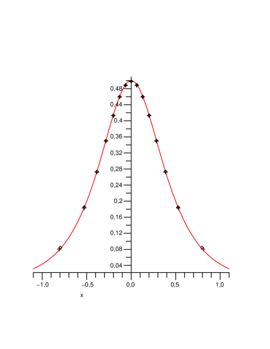
Figure 4: Numerical vs analytical densities for $gl(2)$ alternating $(s=\frac{1}{2},s=\frac{3}{2})$ spin chain

where $\lambda_{k}$ are the ordered solutions. Since the densities are computed thanks to the monotony hypothesis, the matching between them and their discrete analogues confirms the hypothesis, at least for the vacuum state (see figure 4).

This hypothesis allows us to get the bounds on $Q_{m,k}^{(j)}$ sending $\lambda_{m,k}^{(j)}$ to $\pm\infty$. A direct calculation shows that

$$\Phi_{2}^{(p,m)}(\pm\infty)=\pm\pi\,\Big{(}4\,\min(m,p)+2-\delta_{m,p}\Big{)}\quad;\quad\Phi_{-1}^{(p,m)}(\pm\infty)=\mp\pi\,\Big{(}2\,\min(m,p)+1\Big{)}\qquad$$ (3.26)

$$\Phi_{a}^{(m)}(\pm\infty)=\pm\pi\,\min(2m+1,a)$$ (3.27)

and for $j=1,\ldots,N$, $m\in\frac{1}{2}{\mathbb{Z}}_{+}$:

$$Q^{(j)}_{m,\pm\infty}=\pm\frac{1}{2}\Big{(}\nu^{(j)}_{m}+4m+1+\sum_{\ell=1}^{L}\delta_{j,j_{\ell}}\,\min(2m+1,a_{\ell})-\sum_{n\in\frac{1}{2}{\mathbb{Z}}_{+}}\min(2m+1,2n+1)\,w_{n}^{(j)}\Big{)}\quad$$ (3.28)

where we have introduced

$$w_{m}^{(j)}=2\nu^{(j)}_{m}-\nu^{(j-1)}_{m}-\nu^{(j+1)}_{m}$$ (3.29)

with the convention $w_{m}^{(0)}=w_{m}^{(N+1)}=0$, $\forall m\in\frac{1}{2}{\mathbb{Z}}_{+}$.

The reached bounds are deduced from the limiting values $Q^{(j)}_{m,\pm\infty}$ shifting them by the length of a string:

$$Q^{(j)}_{m,\min}=Q^{(j)}_{m,-\infty}+2m+1\hskip 11.38109pt\mbox{and}\hskip 11.38109ptQ^{(j)}_{m,\max}=Q^{(j)}_{m,+\infty}-(2m+1)$$ (3.30)

Since we assumed the monotony hypothesis, all the $Q^{(j)}_{m,k}$, for $j$ and $m$ fixed, are different one from each other. Then, the above bounds, which indicate the possible values for the $Q^{(j)}_{m,k}$, also show, through combinatorics, the maximal number of possible states. It is thus natural to introduce:

Definition 3.2

For a given state, the valence of the length $2m+1$ string in the $j$ sea is defined by $P_{m}^{(j)}=Q^{(j)}_{m,\max}-Q^{(j)}_{m,\min}+1$, that is:

$$P_{m}^{(j)}=\nu_{m}^{(j)}-\sum_{n\in\frac{1}{2}{\mathbb{Z}}_{+}}\Big{\{}\min(2m+1,2n+1)\,w_{n}^{(j)}\Big{\}}+\sum_{l=1}^{L}\delta_{j,j_{l}}\,\min(2m+1,a_{\ell})$$ (3.31)

where the representation at site $l$ is given by the $sl(N)$ weight $(\underbrace{0,\ldots,0}_{j_{l}-1},a_{l},0,\ldots,0)$ and the coefficients $w_{n}^{(j)}$ are given in equation (3.29).

We can reformulate the spin (2.29) of these states as

$$S_{j}=-\sum_{n\in\frac{1}{2}{\mathbb{Z}}_{+}}(2n+1)\,w_{n}^{(j)}+\sum_{l=1}^{L}\delta_{j,j_{l}}\,a_{l}$$ (3.32)

We illustrate this definition with the previous three examples.

Examples

1. For instance, the valences corresponding to a fundamental $sl(N)$ spin chain are given by

   $$P_{m}^{(1)} = \nu_{m}^{(1)}-\sum_{n\in\frac{1}{2}{\mathbb{Z}}_{+}}\Big{\{}\min(2m+1,2n+1)\,w_{n}^{(1)}\Big{\}}+L$$ (3.33)

   $$P_{m}^{(j)} = \nu_{m}^{(j)}-\sum_{n\in\frac{1}{2}{\mathbb{Z}}_{+}}\Big{\{}\min(2m+1,2n+1)\,w_{n}^{(j)}\Big{\}}\hskip 11.38109pt\mbox{for}\hskip 11.38109pt1<j\leq N$$ (3.34)

2. The valences for a $sl(2)$ spin-s chain are

   $$P_{m}=\nu_{m}-\sum_{n\in\frac{1}{2}{\mathbb{Z}}_{+}}\,\min(2m+1,2n+1)\,\nu_{n}+L\,\min(2m+1,s)$$ (3.35)

3. The valences for an alternating $sl(N)$ spin chain are given by

   $$P_{m}^{(j_{1})} = \nu_{m}^{(j_{1})}-\sum_{n\in\frac{1}{2}{\mathbb{Z}}_{+}}\Big{\{}\min(2m+1,2n+1)\,w_{n}^{(j_{1})}\Big{\}}+\frac{L}{2}\,\min(2m+1,a_{1})$$ (3.36)

   $$P_{m}^{(j_{2})} = \nu_{m}^{(j_{2})}-\sum_{n\in\frac{1}{2}{\mathbb{Z}}_{+}}\Big{\{}\min(2m+1,2n+1)\,w_{n}^{(j_{2})}\Big{\}}+\frac{L}{2}\,\min(2m+1,a_{2})$$ (3.37)

   $$P_{m}^{(j)} = \nu_{m}^{(j)}-\sum_{n\in\frac{1}{2}{\mathbb{Z}}_{+}}\Big{\{}\min(2m+1,2n+1)\,w_{n}^{(j)}\Big{\}}\hskip 11.38109pt\mbox{for}\hskip 11.38109ptj\neq j_{1},j_{2}$$ (3.38)

   where we have supposed $j_{1}\neq j_{2}$.

   When $j_{1}=j_{2}\equiv j_{0}$ (and $a_{1}\neq a_{2}$), the valences read

   $$P_{m}^{(j_{0})} = \nu_{m}^{(j_{0})}-\sum_{n\in\frac{1}{2}{\mathbb{Z}}_{+}}\Big{\{}\min(2m+1,2n+1)\,w_{n}^{(j_{0})}\Big{\}}+\frac{L}{2}\,\Big{(}\min(2m+1,a_{1})+\min(2m+1,a_{2})\Big{)}$$

   $$P_{m}^{(j)} = \nu_{m}^{(j)}-\sum_{n\in\frac{1}{2}{\mathbb{Z}}_{+}}\Big{\{}\min(2m+1,2n+1)\,w_{n}^{(j)}\Big{\}}\hskip 11.38109pt\mbox{for}\hskip 11.38109ptj\neq j_{0}$$

4 Vacuum states

In this section, we look for states that correspond to zero excitation (no hole) configuration, i.e.

$$P_{m}^{(j)}=\nu_{m}^{(j)}\,,\ \forall j=1,\ldots,N-1\hskip 11.38109pt\mbox{and}\hskip 11.38109ptm\in\frac{1}{2}{\mathbb{Z}}_{+}.$$ (4.1)

We call them vacuum states. We have the following theorem:

Theorem 4.1

We consider a spin chain based on $gl(N)$, with on each site $\ell$, a representation given by the Young tableau fig. 1, characterized by $(a_{\ell},j_{\ell})$.
(i) For such a spin chain, the vacuum state is non-degenerate, and built on $\nu_{m}^{(j)}$ strings of length $(2m+1)$ in the $j$ sea, with

$$N\,\nu_{m}^{(j)}=\sum_{l=1}^{L}\delta_{2m+1,a_{l}}\,\min(j,j_{l})\,\Big{(}N-\max(j,j_{l})\Big{)}$$ (4.2)

(ii) The vacuum state is antiferromagnetic, i.e. it is a spin 0 state under the $sl(N)$ symmetry algebra of the transfer matrix.

Proof: The vacuum states are defined by $P_{m}^{(j)}=\nu_{m}^{(j)}$, $\forall j=1,\ldots,N-1$ and $m\in\frac{1}{2}{\mathbb{Z}}_{+}$, hence they must solve the equations

$$\sum_{n\in\frac{1}{2}{\mathbb{Z}}_{+}}\Big{\{}\min(2m+1,2n+1)\,w_{n}^{(j)}\Big{\}}=\sum_{l=1}^{L}\delta_{j,j_{l}}\,\,\min(a_{l},2m+1)$$ (4.3)

$$\forall j=1,\ldots,N-1\hskip 11.38109pt\mbox{and}\hskip 11.38109ptm\in\frac{1}{2}{\mathbb{Z}}_{+}$$

Performing the difference of two equations (4.3), for $m$ and $m+\frac{1}{2}$, and using the identities

$$\min(a_{l},2m+1)=a_{l}\,\theta(2m\geq a_{l})+(2m+1)\,\theta(a_{l}>2m)$$ (4.4)

$$\theta(2m+1\geq a_{l})-\theta(2m\geq a_{l})=\delta_{2m+1,a_{l}}$$ (4.5)

$$\theta(2m<a_{l})-\theta(2m+1<a_{l})=\delta_{2m+1,a_{l}}$$ (4.6)

one gets

$$\sum_{n>m}\,w_{n}^{(j)}=\sum_{l=1}^{L}\delta_{j,j_{l}}\,\theta(a_{l}>2m+1)\,.$$ (4.7)

This proves that the system (4.3) is triangular, and thus admits at most one solution, so that one has only to prove the existence of such a state.

We take the values:

$$w_{m}^{(j)}=\sum_{l=1}^{L}\delta_{j,j_{l}}\,\delta_{a_{l},2m+1}$$ (4.8)

Pluging these values into (4.3), a direct calculation shows that these equations are all satisfied. Hence, (4.8) defines a vacuum state.

Rewriting the expression (4.8) in terms of $\nu_{m}^{(j)}$ using (3.29), we get the result (4.2).

Using the values (4.8) and the expression (3.32), it is then easy to compute that the $sl(N)$ eigenvalues of these states vanish.  

Remark 4.1

Note that the relation (4.2) implies that $\sum_{l=1}^{L}\delta_{2m+1,a_{l}}\,\min(j,j_{l})\,(N-\max(j,j_{l}))$ must be a multiple of $N$. This constraint (on the existence of the vacuum state) can be viewed as a constraint on the length of the spin chain, with parameters $a_{l}$ and $j_{l}$, see examples below.

In words, the above theorem states that the vacuum state is built with strings of length $a_{\ell}$ in each sea. The number of these strings in the sea $j$ is a function of $j$ and $j_{\ell}$, $\ell=1,\ldots,L$.

Even though the construction of Hamiltonian for a general choice of representation is difficult and not in the scope of this work, we may expect that for an approriate choice of the coupling constants the spin chain becomes a bipartite lattice ($L_{0}\geq 2$). In this case, the Marshall’s theorem [36, 37] can be applied and the state found in the theorem 4.1 is the ground state for the corresponding Hamiltonian.

Examples

1. For instance, the vacuum state corresponding to a fundamental $sl(N)$ spin chain is given by

   $$\nu_{0}^{(j)}=\frac{L(N-j)}{N}\hskip 11.38109pt\mbox{and}\hskip 11.38109pt\nu_{n}^{(j)}=0\,,\ \forall\,n\in\frac{1}{2}{\mathbb{Z}}_{>0}\,,\qquad 1\leq j\leq N-1\,.$$ (4.9)

   One recovers the usual antiferromagnetic ground state, with only real Bethe roots. Their total number is $\frac{L(N-j)}{N}$, so that the state exists only if $L(N-j)$ can be divided by $N$, i.e. $L$ multiple of $N$.

2. For a $sl(2)$ spin-s chain we get

   $$\nu_{s-\frac{1}{2}}=\frac{L}{2}\hskip 11.38109pt\mbox{and}\hskip 11.38109pt\nu_{n}=0\,,\ \forall\,n\in\frac{1}{2}{\mathbb{Z}}\,,\ n\neq s-\frac{1}{2}\,.$$ (4.10)

   We get $\frac{L}{2}$ strings of length $2s$, as expected for the ground state. One also recovers that $L$ must be even.

3. If one considers an alternating $sl(N)$ spin chain ​​, one gets for $n\in\frac{1}{2}{\mathbb{Z}}$

   $$\nu_{n}^{(j)}=0\hskip 11.38109pt\mbox{when}\hskip 11.38109ptn\neq n_{1}=\frac{a_{1}-1}{2}\hskip 11.38109pt\mbox{and}\hskip 11.38109ptn\neq n_{2}=\frac{a_{2}-1}{2}\,.$$ (4.11)

   If one supposes furthermore that $a_{1}\neq a_{2}$,

   $$\nu_{n_{k}}^{(j)}=\left\{\begin{array}[]{l}\displaystyle\frac{Lj(N-j_{k})}{2N}\hskip 11.38109pt\mbox{for}\hskip 11.38109ptj\leq j_{k}\\[9.04166pt] \displaystyle\frac{Lj_{k}(N-j)}{2N}\hskip 11.38109pt\mbox{for}\hskip 11.38109ptj\geq j_{k}\end{array}\right.\qquad\ k=1,2$$ (4.12)

5 Thermodynamical limit

The Bethe equations cannot be solved in general however interesting features of the system can be obtained in the thermodynamical limit (i.e. $L\to\infty$). We will need the following definition:

Definition 5.1

A spin chain is called $L_{0}$-regular $(L_{0}\in{\mathbb{Z}}_{+})$ when the types of representations entering in its definition satisfy

$$j_{\ell+L_{0}}=j_{\ell}\hskip 11.38109pt\mbox{and}\hskip 11.38109pta_{\ell+L_{0}}=a_{\ell}\quad,\quad\forall\ell=1,\ldots L\;.$$ (5.1)

The set of integers $\{\bar{a}_{1},\ldots,\bar{a}_{\cal L}\}$ corresponds to the distinct values in the set $\{a_{\ell}|1\leq\ell\leq L_{0}\}$ (let us stress that ${\cal L}$ can be different from $L_{0}$). Finally, we introduce

$${\cal N}=\{n_{\alpha}=\frac{\bar{a}_{\alpha}-1}{2}\;|\;1\leq\alpha\leq{\cal L}\}\;.$$ (5.2)

We also introduce the sets of indices defined by:

$$I_{\alpha}=\{j\in[1,L_{0}]\hskip 11.38109pt\mbox{s.t.}\hskip 11.38109pta_{j}=\bar{a}_{\alpha}\}\ ,\ \forall\alpha\in[1,{\cal L}]$$ (5.3)

such that

$$\sum_{\ell=1}^{L_{0}}\,(\ldots)_{\ell}\ =\ \sum_{\alpha=1}^{{\cal L}}\,\sum_{\ell^{\prime}\in I_{\alpha}}\,(\ldots)_{\ell^{\prime}}\;.$$ (5.4)

The cardinal $|I_{\alpha}|$ corresponds to the multiplicity of $\bar{a}_{\alpha}$ within a subset of $L_{0}$ sites.

Examples

1. For a fundamental $sl(N)$ spin chain ​​, we recall that $a_{\ell}=j_{\ell}=1$ and thus one has $L_{0}=1={\cal L}$, ${\cal N}=\{0\}$ and $I_{1}=\{1\}$.

2. For a $sl(2)$ spin-s chain ​​, we get $a_{\ell}=2s$, $j_{\ell}=1$ and one has $L_{0}=1={\cal L}$, ${\cal N}=\{s-\frac{1}{2}\}$ and $I_{1}=\{1\}$.

3. For an alternating $sl(N)$ spin chain ​​, one has $L_{0}=2={\cal L}$ if $a_{1}\neq a_{2}$ (whatever the two values $j_{1}$ and $j_{2}$ are); while $L_{0}=2$ and ${\cal L}=1$ if $a_{1}=a_{2}$ and $j_{1}\neq j_{2}$. We have ${\cal N}=\{\frac{a_{1}-1}{2},\frac{a_{2}-1}{2}\}$ and $I_{1}=\{1\}$, $I_{2}=\{2\}$ in the first case; ${\cal N}=\{\frac{a_{1}-1}{2}\}$ and $I_{1}=\{1,2\}$ in the second case.

From now on, we assume that the spin chain is $L_{0}$-regular. Then, adding the constraint on the existence of a vacuum state (see remark 4.1) to the above regularity condition, one is led to take $L=p\,N\,L_{0}$, $p\in{\mathbb{Z}}_{+}$.

5.1 Regularity and constraint on representations

The regularity hypothesis is also a natural assumption to solve the constraint (3.10) within the $L\to\infty$ limit. Indeed, this constraint applied to a regular spin chain is equivalent to

$$\sum_{\ell=1}^{L_{0}}\left(\gamma^{(j)}_{\ell}+\frac{a^{(j)}_{\ell}}{2}\right)^{2p}\,=\,\sum_{\ell=1}^{L_{0}}\left(\gamma^{(j)}_{\ell}-\frac{a^{(j)}_{\ell}}{2}\right)^{2p}\,,\quad 1\leq p\leq L_{0}$$ (5.5)

which is not affected by the limit.

As already remarked, in the case of $gl(2)$, the representations (3.16) describe all the representations, so that there is in fact no constraint for this algebra (whatever the value of $L_{0}$). Then, it is natural to wonder if other kinds of representations can appear when $N>2$.

When $L_{0}=1$, a direct calculation proves that the constraint (5.5) is equivalent to the equation (3.15), so that the representations described by (3.16) are the only ones compatible with the string hypothesis (whatever the value of $N$).

For $L_{0}=2$, one can solve directly the equations (5.5). One finds that $a^{(j)}_{\ell}\geq 0$ and $\gamma^{(j)}_{\ell}$ must fulfil one of the conditions (for $j=1,\ldots,N-1$):

$$\begin{cases}a^{(j)}_{1}\,\gamma^{(j)}_{1}=0\hskip 11.38109pt\mbox{and}\hskip 11.38109pta^{(j)}_{2}\,\gamma^{(j)}_{2}=0\\ \hskip 11.38109pt\mbox{or}\hskip 11.38109pt\\ a^{(j)}_{1}=2\,\epsilon^{(j)}\,\gamma^{(j)}_{2}\hskip 11.38109pt\mbox{and}\hskip 11.38109pta^{(j)}_{2}=-2\,\epsilon^{(j)}\,\gamma^{(j)}_{1}\,,\quad\epsilon^{(j)}=\pm 1\,,\\ \hskip 11.38109pt\mbox{or}\hskip 11.38109pt\\ a^{(j)}_{1}=a^{(j)}_{2}\hskip 11.38109pt\mbox{and}\hskip 11.38109pt\gamma^{(j)}_{2}=-\gamma^{(j)}_{1}\,.\end{cases}$$ (5.6)

Remark that the first line (when applied for all $j$) corresponds to the representations we have studied in the present paper. Plugging the value (3.11) of $\gamma^{(j)}_{\ell}$, one gets

$$\begin{cases}a^{(j)}_{1}\,\Big{(}2\,\theta_{1}+\varpi^{(j)}_{1}+\varpi^{(j+1)}_{1}-j\Big{)}=0\hskip 11.38109pt\mbox{and}\hskip 11.38109pta^{(j)}_{2}\,\Big{(}2\,\theta_{2}+\varpi^{(j)}_{2}+\varpi^{(j+1)}_{2}-j\Big{)}=0\,,\\ \hskip 11.38109pt\mbox{or}\hskip 11.38109pt\\ 2\,\theta_{2}=\epsilon^{(j)}\,a^{(j)}_{1}-(\varpi^{(j)}_{2}+\varpi^{(j+1)}_{2})+j\hskip 11.38109pt\mbox{and}\hskip 11.38109pt2\,\theta_{1}=-\epsilon^{(j)}\,a^{(j)}_{2}-(\varpi^{(j)}_{1}+\varpi^{(j+1)}_{1})+j\,,\\ \hskip 11.38109pt\mbox{or}\hskip 11.38109pt\\ a^{(j)}_{1}=a^{(j)}_{2}\hskip 11.38109pt\mbox{and}\hskip 11.38109pt2\,(\theta_{1}+\theta_{2})=2\,j-(\varpi^{(j)}_{1}+\varpi^{(j+1)}_{1}+\varpi^{(j)}_{2}+\varpi^{(j+1)}_{2})\,,\end{cases}$$ (5.7)

that one needs to solve in $\theta_{\ell}$, $a^{(j)}_{\ell}=\varpi^{(j)}_{\ell}-\varpi^{(j+1)}_{\ell}$ and $\varpi^{(1)}_{\ell}$, with the conditions $a^{(j)}_{\ell}\geq 0$. This is still an intriguing problem, and we just give the complete classification of solutions for $N=3$ (obtained by direct calculation).

In the case of $sl(3)$, and discarding the case of arbitrary rectangular Young tableaux on each site, we get eight classes of solutions, which reduce to four taking into account the symmetry between the two sites. In each case, one site is represented by a general Young tableau $(b,c)$, while the second one is rectangular $(a,0)$ or $(0,a)$, but with $a$ determined by $b$ and $c$. We present in figure 2 the Young tableaux of the different cases. As previously, the inhomogeneity parameters and the $gl(1)$ parameters are constrained:

$$\theta_{1}+\varpi_{1}^{(1)}=\frac{1}{2}(b+1)+c+1\hskip 11.38109pt\mbox{and}\hskip 11.38109pt\theta_{2}+\varpi_{2}^{(1)}=\frac{1}{2}(b+1)\,.$$ (5.8)

$$(c,b)\qquad\begin{picture}(60.0,30.0)\put(0.0,20.0){\line(1,0){10.0}}\put(20.0,20.0){\line(1,0){10.0}}\put(50.0,20.0){\line(1,0){10.0}} \put(0.0,10.0){\line(1,0){10.0}}\put(20.0,10.0){\line(1,0){10.0}}\put(50.0,10.0){\line(1,0){10.0}} \put(0.0,0.0){\line(1,0){10.0}}\put(20.0,0.0){\line(1,0){10.0}} \put(0.0,0.0){\line(0,1){20.0}}\put(10.0,0.0){\line(0,1){20.0}} \put(20.0,0.0){\line(0,1){20.0}}\put(30.0,0.0){\line(0,1){20.0}} \put(50.0,20.0){\line(0,-1){10.0}}\put(60.0,20.0){\line(0,-1){10.0}} \put(30.0,20.0){\line(1,0){2.0}}\put(34.0,20.0){\line(1,0){2.0}}\put(38.0,20.0){\line(1,0){2.0}}\put(42.0,20.0){\line(1,0){2.0}}\put(46.0,20.0){\line(1,0){2.0}}\put(50.0,20.0){\line(1,0){2.0}}\put(54.0,20.0){\line(1,0){2.0}}\put(58.0,20.0){\line(1,0){2.0}} \put(30.0,10.0){\line(1,0){2.0}}\put(34.0,10.0){\line(1,0){2.0}}\put(38.0,10.0){\line(1,0){2.0}}\put(42.0,10.0){\line(1,0){2.0}}\put(46.0,10.0){\line(1,0){2.0}}\put(50.0,10.0){\line(1,0){2.0}}\put(54.0,10.0){\line(1,0){2.0}}\put(58.0,10.0){\line(1,0){2.0}} \put(10.0,0.0){\line(1,0){2.0}}\put(14.0,0.0){\line(1,0){2.0}}\put(18.0,0.0){\line(1,0){2.0}} \put(10.0,10.0){\line(1,0){2.0}}\put(14.0,10.0){\line(1,0){2.0}}\put(18.0,10.0){\line(1,0){2.0}} \put(10.0,20.0){\line(1,0){2.0}}\put(14.0,20.0){\line(1,0){2.0}}\put(18.0,20.0){\line(1,0){2.0}} \put(2.0,-3.0){$\underbrace{~{}~{}~{}~{}~{}~{}~{}}_{\displaystyle b}$} \put(32.0,7.0){$\underbrace{~{}~{}~{}~{}~{}~{}~{}}_{\displaystyle c}$} \end{picture} \begin{picture}(60.0,30.0)\put(0.0,10.0){\line(1,0){20.0}}\put(50.0,10.0){\line(1,0){10.0}} \put(0.0,0.0){\line(1,0){20.0}}\put(50.0,0.0){\line(1,0){10.0}} \put(0.0,10.0){\line(0,-1){10.0}}\put(50.0,10.0){\line(0,-1){10.0}} \put(10.0,10.0){\line(0,-1){10.0}}\put(60.0,10.0){\line(0,-1){10.0}} \put(20.0,10.0){\line(0,-1){10.0}} \put(20.0,10.0){\line(1,0){2.0}}\put(24.0,10.0){\line(1,0){2.0}}\put(28.0,10.0){\line(1,0){2.0}}\put(32.0,10.0){\line(1,0){2.0}}\put(36.0,10.0){\line(1,0){2.0}}\put(40.0,10.0){\line(1,0){2.0}}\put(44.0,10.0){\line(1,0){2.0}}\put(48.0,10.0){\line(1,0){2.0}} \put(20.0,0.0){\line(1,0){2.0}}\put(24.0,0.0){\line(1,0){2.0}}\put(28.0,0.0){\line(1,0){2.0}}\put(32.0,0.0){\line(1,0){2.0}}\put(36.0,0.0){\line(1,0){2.0}}\put(40.0,0.0){\line(1,0){2.0}}\put(44.0,0.0){\line(1,0){2.0}}\put(48.0,0.0){\line(1,0){2.0}} \put(0.0,-3.0){$\underbrace{~{}~{}~{}~{}~{}~{}~{}~{}~{}~{}~{}~{}~{}~{}~{}}_{\displaystyle c}$} \end{picture}\qquad(c,0)$$

$$(b,c)\qquad\begin{picture}(60.0,30.0)\put(0.0,20.0){\line(1,0){10.0}}\put(20.0,20.0){\line(1,0){10.0}}\put(50.0,20.0){\line(1,0){10.0}} \put(0.0,10.0){\line(1,0){10.0}}\put(20.0,10.0){\line(1,0){10.0}}\put(50.0,10.0){\line(1,0){10.0}} \put(0.0,0.0){\line(1,0){10.0}}\put(20.0,0.0){\line(1,0){10.0}} \put(0.0,0.0){\line(0,1){20.0}}\put(10.0,0.0){\line(0,1){20.0}} \put(20.0,0.0){\line(0,1){20.0}}\put(30.0,0.0){\line(0,1){20.0}} \put(50.0,20.0){\line(0,-1){10.0}}\put(60.0,20.0){\line(0,-1){10.0}} \put(30.0,20.0){\line(1,0){2.0}}\put(34.0,20.0){\line(1,0){2.0}}\put(38.0,20.0){\line(1,0){2.0}}\put(42.0,20.0){\line(1,0){2.0}}\put(46.0,20.0){\line(1,0){2.0}}\put(50.0,20.0){\line(1,0){2.0}}\put(54.0,20.0){\line(1,0){2.0}}\put(58.0,20.0){\line(1,0){2.0}} \put(30.0,10.0){\line(1,0){2.0}}\put(34.0,10.0){\line(1,0){2.0}}\put(38.0,10.0){\line(1,0){2.0}}\put(42.0,10.0){\line(1,0){2.0}}\put(46.0,10.0){\line(1,0){2.0}}\put(50.0,10.0){\line(1,0){2.0}}\put(54.0,10.0){\line(1,0){2.0}}\put(58.0,10.0){\line(1,0){2.0}} \put(10.0,0.0){\line(1,0){2.0}}\put(14.0,0.0){\line(1,0){2.0}}\put(18.0,0.0){\line(1,0){2.0}} \put(10.0,10.0){\line(1,0){2.0}}\put(14.0,10.0){\line(1,0){2.0}}\put(18.0,10.0){\line(1,0){2.0}} \put(10.0,20.0){\line(1,0){2.0}}\put(14.0,20.0){\line(1,0){2.0}}\put(18.0,20.0){\line(1,0){2.0}} \put(2.0,-3.0){$\underbrace{~{}~{}~{}~{}~{}~{}~{}}_{\displaystyle c}$} \put(32.0,7.0){$\underbrace{~{}~{}~{}~{}~{}~{}~{}}_{\displaystyle b}$} \end{picture} \begin{picture}(60.0,30.0)\put(0.0,20.0){\line(1,0){20.0}}\put(50.0,20.0){\line(1,0){10.0}} \put(0.0,10.0){\line(1,0){20.0}}\put(50.0,10.0){\line(1,0){10.0}} \put(0.0,0.0){\line(1,0){20.0}}\put(50.0,0.0){\line(1,0){10.0}} \put(0.0,0.0){\line(0,1){20.0}}\put(50.0,0.0){\line(0,1){20.0}} \put(10.0,0.0){\line(0,1){20.0}}\put(60.0,0.0){\line(0,1){20.0}} \put(20.0,0.0){\line(0,1){20.0}} \put(20.0,20.0){\line(1,0){2.0}}\put(24.0,20.0){\line(1,0){2.0}}\put(28.0,20.0){\line(1,0){2.0}}\put(32.0,20.0){\line(1,0){2.0}}\put(36.0,20.0){\line(1,0){2.0}}\put(40.0,20.0){\line(1,0){2.0}}\put(44.0,20.0){\line(1,0){2.0}}\put(48.0,20.0){\line(1,0){2.0}} \put(20.0,10.0){\line(1,0){2.0}}\put(24.0,10.0){\line(1,0){2.0}}\put(28.0,10.0){\line(1,0){2.0}}\put(32.0,10.0){\line(1,0){2.0}}\put(36.0,10.0){\line(1,0){2.0}}\put(40.0,10.0){\line(1,0){2.0}}\put(44.0,10.0){\line(1,0){2.0}}\put(48.0,10.0){\line(1,0){2.0}} \put(20.0,0.0){\line(1,0){2.0}}\put(24.0,0.0){\line(1,0){2.0}}\put(28.0,0.0){\line(1,0){2.0}}\put(32.0,0.0){\line(1,0){2.0}}\put(36.0,0.0){\line(1,0){2.0}}\put(40.0,0.0){\line(1,0){2.0}}\put(44.0,0.0){\line(1,0){2.0}}\put(48.0,0.0){\line(1,0){2.0}} \put(0.0,-3.0){$\underbrace{~{}~{}~{}~{}~{}~{}~{}~{}~{}~{}~{}~{}~{}~{}~{}}_{\displaystyle c}$} \end{picture}\qquad(0,c)$$

Figure 2: The remaining allowed representations for $L_{0}=2$ and $N=3$

5.2 Limit of the Bethe equations for the vacuum

For vacuum states, using the values (3.30) of $Q_{m,\min}^{(j)}$ and $Q_{m,\max}^{(j)}$ and the monotony of the $Q$’s, one gets

$$Q_{m,k}^{(j)}=k-\frac{1}{2}(\nu_{m}^{(j)}+1)\,\quad k=1,\ldots,\nu_{m}^{(j)}.$$ (5.9)

Using the regularity hypothesis and equation (5.4), we simplify the BAE (3.24) to:

$$\sum_{n\in{\cal N}}\left\{\sum_{\ell=1}^{\nu^{(j-1)}_{n}}\Phi_{-1}^{(m,n)}(\lambda_{m,k}^{(j)}-\lambda_{n,\ell}^{(j-1)})+\sum_{\genfrac{}{}{0.0pt}{}{\ell=1}{(n,\ell)\neq(m,k)}}^{\nu^{(j)}_{n}}\Phi_{2}^{(m,n)}(\lambda_{m,k}^{(j)}-\lambda_{n,\ell}^{(j)})+\sum_{\ell=1}^{\nu^{(j+1)}_{n}}\Phi_{-1}^{(m,n)}(\lambda_{m,k}^{(j)}-\lambda_{n,\ell}^{(j+1)})\right\}$$

$$=-2\pi Q^{(j)}_{m,k}+\frac{L}{L_{0}}\sum_{\alpha=1}^{{\cal L}}\Big{(}\sum_{\ell\in I_{\alpha}}\delta_{j,j_{\ell}}\Big{)}\,\Phi_{\bar{a}_{\alpha}}^{(m)}(\lambda_{m,k}^{(j)})$$ (5.10)

$$\qquad\forall k=1,\ldots,\nu^{(j)}_{m}\ ,\ \forall j=1,\ldots,N-1\ ,\ \forall m\in\frac{1}{2}{\mathbb{Z}}_{+}$$

Note that we can restrict ourself to the cases $m\in{\cal N}$, keeping in mind that $\nu_{m}^{(j)}=0$ when $m\not\in{\cal N}$.

In the thermodynamical limit $L\to\infty$, $Q_{m,k}^{(j)}/L$ becomes a continuous variable $x$, whose bounds are obtained from (5.9) and (4.2):

$$-Y_{m}^{(j)}\leq x\leq Y_{m}^{(j)}\hskip 11.38109pt\mbox{with}\hskip 11.38109ptY_{m}^{(j)}=\frac{1}{2NL_{0}}\,\sum_{\ell=1}^{L_{0}}\delta_{2m+1,a_{\ell}}\,\min(j,j_{\ell})\,\Big{(}N-\max(j,j_{\ell})\Big{)}\;.$$ (5.11)

Then, the thermodynamical limit of the BAE reads

$$\sum_{n\in{\cal N}}\left\{\int_{-Y_{n}^{(j-1)}}^{Y_{n}^{(j-1)}}dy\ \Phi_{-1}^{(m,n)}(\lambda_{m}^{(j)}(x)-\lambda_{n}^{(j-1)}(y))+\int_{-Y_{n}^{(j)}}^{Y_{n}^{(j)}}dy\ \Phi_{2}^{(m,n)}(\lambda_{m}^{(j)}(x)-\lambda_{n}^{(j)}(y))\right.$$

$$\qquad\left.+\int_{-Y_{n}^{(j+1)}}^{Y_{n}^{(j+1)}}dy\ \Phi_{-1}^{(m,n)}(\lambda_{m}^{(j)}(x)-\lambda_{n}^{(j+1)}(y))\right\}\ =\ -2\pi\,x+\frac{1}{L_{0}}\sum_{\alpha=1}^{{\cal L}}\Big{(}\sum_{\ell\in I_{\alpha}}\delta_{j,j_{\ell}}\Big{)}\,\Phi_{\bar{a}_{\alpha}}^{(m)}(\lambda_{m}^{(j)}(x))\qquad\qquad$$ (5.12)

$$\qquad\forall x\in[-Y_{m}^{(j)}\,,\,Y_{m}^{(j)}]\ ,\ \forall j=1,\ldots,N-1\ ,\ \forall m\in{\cal N}$$

Making the change of variables $x\in[-Y_{m}^{(j)}\,,\,Y_{m}^{(j)}]\to\lambda_{m}^{(j)}(x)\in]-\infty\,,\,\infty[$, we get

$$\sum_{n\in{\cal N}}\left\{\int_{-\infty}^{\infty}d\lambda\,\sigma_{n}^{(j-1)}(\lambda)\,{\Phi_{-1}^{(m,n)}}(\lambda_{0}-\lambda)+\int_{-\infty}^{\infty}d\lambda\,\sigma_{n}^{(j)}(\lambda)\,{\Phi_{2}^{(m,n)}}(\lambda_{0}-\lambda)\right.$$

$$\qquad\left.+\int_{-\infty}^{\infty}d\lambda\,\sigma_{n}^{(j+1)}(\lambda)\,{\Phi_{-1}^{(m,n)}}(\lambda_{0}-\lambda)\right\}\ =\ -2\pi\,x(\lambda_{0})+\frac{1}{L_{0}}\sum_{\alpha=1}^{{\cal L}}\Big{(}\sum_{\ell\in I_{\alpha}}\delta_{j,j_{\ell}}\Big{)}\,\Phi_{\bar{a}_{\alpha}}^{(m)}(\lambda_{0})\qquad\qquad$$ (5.13)

$$\qquad\forall\lambda_{0}\in\;]-\infty\,,\,\infty[\ ,\ \forall j=1,\ldots,N-1\ ,\ \forall m\in{\cal N}$$

where $\lambda_{0}$ stands for $\lambda_{m}^{(j)}(x)$, and $\sigma_{n}^{(j)}=dx/d\lambda_{n}^{(j)}$.

5.3 Calculation of the densities

To solve these equations, one performs a differentiation w.r.t. $\lambda_{m}^{(j)}$ and a Fourier transform. One computes:

$$\Psi^{(m,n)}_{-1}(\lambda)=\frac{d\Phi^{(m,n)}_{-1}(\lambda)}{d\lambda} = -2\,\sum_{s=|m-n|}^{m+n}\frac{s+\frac{1}{2}}{(s+\frac{1}{2})^{2}+\lambda^{2}}$$ (5.14)

$$\Psi^{(m,n)}_{2}(\lambda)=\frac{d\Phi^{(m,n)}_{2}(\lambda)}{d\lambda} = 2\,\left(\frac{m+n+1}{(m+n+1)^{2}+\lambda^{2}}+\frac{|m-n|}{(m-n)^{2}+\lambda^{2}}+2\sum_{s=|m-n|+1}^{m+n}\frac{s}{s^{2}+\lambda^{2}}\right)\quad$$ (5.15)

$$\Psi^{(m)}_{a}(\lambda)=\frac{d\Phi^{(m)}_{a}(\lambda)}{d\lambda} = 2\,\sum_{s=|\frac{a}{2}-m|+1}^{\frac{a}{2}+m}\frac{s}{s^{2}+\lambda^{2}}+2\;\theta(\frac{a}{2}>m)\;\frac{\frac{a}{2}-m}{(\frac{a}{2}-m)^{2}+\lambda^{2}}$$ (5.16)

We normalize the Fourier transform as:

$$\widehat{f}(p)=\frac{1}{2\pi}\int_{-\infty}^{\infty}e^{ip\lambda}\;f(\lambda)\;d\lambda\,.$$ (5.17)

Explicitly, one finds:

$$\widehat{\Psi}^{(m,n)}_{-1}(p) = -\,\exp\Big{(}-|p|\big{(}\max(m,n)+\frac{1}{2}\big{)}\Big{)}\;\frac{\sinh\Big{(}|p|\big{(}\min(m,n)+\frac{1}{2}\big{)}\Big{)}}{\sinh\frac{|p|}{2}}$$ (5.18)

$$\widehat{\Psi}^{(m,n)}_{2}(p) = -2\,\cosh\frac{|p|}{2}\;\widehat{\Psi}^{(m,n)}_{-1}(p)-\delta_{m,n}\qquad$$ (5.19)

$$\widehat{\Psi}^{(m)}_{a}(p) = \exp\Big{(}-|p|\max(\frac{a}{2},m+\frac{1}{2})\Big{)}\;\frac{\sinh\Big{(}|p|(\min(\frac{a}{2},m+\frac{1}{2})\Big{)}}{\sinh\frac{|p|}{2}}$$ (5.20)

We introduce $\widehat{\Psi}(p)$, a $(N-1)\times(N-1)$ matrix of ${\cal L}\times{\cal L}$ blocks:

$$\widehat{\Psi}(p)=\left(\begin{array}[]{cccc}{\mathbb{I}}+\widehat{\Psi}_{2}(p)&\widehat{\Psi}_{-1}(p)&0&0\\ \widehat{\Psi}_{-1}(p)&{\mathbb{I}}+\widehat{\Psi}_{2}(p)&\widehat{\Psi}_{-1}(p)&0\\ &\ddots&\ddots&\\ 0&\widehat{\Psi}_{-1}(p)&{\mathbb{I}}+\widehat{\Psi}_{2}(p)&\widehat{\Psi}_{-1}(p)\\ 0&0&\widehat{\Psi}_{-1}(p)&{\mathbb{I}}+\widehat{\Psi}_{2}(p)\end{array}\right)$$ (5.21)

where the blocks are defined by

$$\widehat{\Psi}_{j}(p)=\left(\begin{array}[]{cccc}\widehat{\Psi}^{(n_{1},n_{1})}_{j}(p)&\widehat{\Psi}^{(n_{1},n_{2})}_{j}(p)&\ldots&\widehat{\Psi}^{(n_{1},n_{{\cal L}})}_{j}(p)\\ \widehat{\Psi}^{(n_{2},n_{1})}_{j}(p)&\widehat{\Psi}^{(n_{2},n_{2})}_{j}(p)&\ldots&\widehat{\Psi}^{(n_{2},n_{{\cal L}})}_{j}(p)\\ \vdots&\ddots&\ddots&\vdots\\ \widehat{\Psi}^{(n_{{\cal L}},n_{1})}_{j}(p)&\widehat{\Psi}^{(n_{{\cal L}},n_{2})}_{j}(p)&\ldots&\widehat{\Psi}^{(n_{{\cal L}},n_{{\cal L}})}_{j}(p)\\ \end{array}\right)\,.$$ (5.22)

In the same way, the BAE’s r.h.s. becomes

$$\Lambda(p)=\frac{1}{L_{0}}\sum_{\alpha=1}^{{\cal L}}\ \sum_{\ell\in I_{\alpha}}\left(\begin{array}[]{c}\delta_{1,j_{\ell}}\\ \delta_{2,j_{\ell}}\\ \vdots\\ \delta_{N-1,j_{\ell}}\end{array}\right)\,\otimes\,\left(\begin{array}[]{c}\widehat{\Psi}^{(n_{1})}_{\bar{a}_{\alpha}}(p)\\ \widehat{\Psi}^{(n_{2})}_{\bar{a}_{\alpha}}(p)\\ \vdots\\ \widehat{\Psi}^{(n_{{\cal L}})}_{\bar{a}_{\alpha}}(p)\end{array}\right)$$ (5.23)

and the (Fourier transformed) unknown variables $\widehat{\sigma}_{n}^{(j)}(p)$ are gathered in the column vector

$$\widehat{\Sigma}(p)=\left(\begin{array}[]{c}\widehat{\Sigma}_{1}(p)\\ \widehat{\Sigma}_{2}(p)\\ \vdots\\ \widehat{\Sigma}_{N-1}(p)\end{array}\right)\hskip 11.38109pt\mbox{with}\hskip 11.38109pt\widehat{\Sigma}_{j}(p)=\left(\begin{array}[]{c}\widehat{\sigma}_{n_{1}}^{(j)}(p)\\ \widehat{\sigma}_{n_{2}}^{(j)}(p)\\ \vdots\\ \widehat{\sigma}_{n_{{\cal L}}}^{(j)}(p)\end{array}\right)\,.$$ (5.24)

Finally, one is led to the following form of the BAE:

$$2\pi\,\widehat{\Psi}(p)\,\widehat{\Sigma}(p)=\Lambda(p)$$ (5.25)

Using the explicit forms of the functions, the matrix $\widehat{\Psi}(p)$ reduces to

$$\widehat{\Psi}(p)={\cal A}(p)\otimes\big{(}-\widehat{\Psi}_{-1}(p)\big{)}\;,\quad{\cal A}(p)=\left(\begin{array}[]{ccccc}2\cosh(\frac{|p|}{2})&-1&0&\ldots&0\\ -1&2\cosh(\frac{|p|}{2})&-1&\ddots&\vdots\\ 0&\ddots&\ddots&\ddots&0\\ \vdots&\ddots&\ \ -1&2\cosh(\frac{|p|}{2})&-1\\ 0&\ldots&0&-1&2\cosh(\frac{|p|}{2})\end{array}\right)$$ (5.26)

with ${\cal A}(p)$ a $(N-1)\times(N-1)$ matrix, reminiscent of the $sl(N)$ Cartan matrix. Let us remark that the matrix ${\cal A}(p)$ is independant of the type of representations.

From this equation, one can deduce the densities $\widehat{\sigma}_{n}^{(j)}(p)$ by inverting the matrix $\widehat{\Psi}(p)$:

$$\widehat{\Sigma}(p)=\frac{1}{2\pi}\,\Big{(}{\cal A}(p)^{-1}\otimes\big{(}-\widehat{\Psi}_{-1}(p)\big{)}^{-1}\Big{)}\;\Lambda(p)$$ (5.27)

where the inverse of the matrix ${\cal A}(p)$ is given by [38]

$$({\cal A}(p)^{-1})_{ij}=\frac{\displaystyle\sinh\Big{(}(N-\max(i,j))\frac{|p|}{2}\Big{)}\;\sinh\Big{(}\min(i,j)\frac{|p|}{2}\Big{)}}{\displaystyle\sinh\Big{(}N\frac{|p|}{2}\Big{)}\;\sinh\Big{(}\frac{|p|}{2}\Big{)}}\;.$$ (5.28)

The previous computations allow us to find a compact expression for the densities given in the following theorem:

Theorem 5.2

Let us consider a $L_{0}$-regular spin chain based on $gl(N)$. For the vacuum, the only non vanishing densities are, for $1\leq k\leq N-1$ and $n_{\alpha}\in{\cal N}$ $(1\leq\alpha\leq{\cal L})$,

$$\sigma^{(k)}_{n_{\alpha}}(\lambda)=\frac{1}{NL_{0}}\sum_{\ell\in I_{\alpha}}\ \ \sum_{q=(|k-j_{\ell}|+1)/2}^{(k+j_{\ell}-1)/2}\quad\frac{\displaystyle\sin\Big{(}\frac{2q\pi}{N}\Big{)}}{\displaystyle\cosh\Big{(}\frac{2\pi}{N}\lambda\Big{)}-\cos\Big{(}\frac{2q\pi}{N}\Big{)}}$$ (5.29)

where the sets $I_{\alpha}$ have been introduced in (5.3).

For the particular case of $gl(2)$ spin chains, the non-vanishing densities further simplify to:

$$\sigma_{s_{\alpha}-\frac{1}{2}}(\lambda)=\frac{|I_{\alpha}|}{2L_{0}}\;\frac{1}{\displaystyle\cosh\pi\lambda},\quad\alpha=1,\ldots,{\cal L}$$ (5.30)

where $s_{\alpha}=n_{\alpha}+\frac{1}{2}$ denote the spins on the chain, and $|I_{\alpha}|$ is the cardinal of $I_{\alpha}$.

Proof: We deduce from relation (5.27) the following expression for the vectors $\widehat{\Sigma}_{i}(p)$ defined in (5.24):

$$\displaystyle\widehat{\Sigma}_{i}(p) = \frac{1}{2\pi\,L_{0}}\sum_{\alpha=1}^{{\cal L}}\ \Big{(}\sum_{\ell\in I_{\alpha}}({\cal A}(p)^{-1})_{i,j_{\ell}}\Big{)}\;\big{(}-\widehat{\Psi}_{-1}(p)\big{)}^{-1}\;\Lambda_{\alpha}(p)$$ (5.31)

with

$$\Lambda_{\alpha}(p)=\left(\begin{array}[]{c}\displaystyle\exp\Big{(}-\frac{|p|}{2}\max(\bar{a}_{\alpha},\bar{a}_{1})\Big{)}\;\frac{\sinh\Big{(}\frac{|p|}{2}(\min(\bar{a}_{\alpha},\bar{a}_{1})\Big{)}}{\sinh\frac{|p|}{2}}\\ \vdots\\ \displaystyle\exp\Big{(}-\frac{|p|}{2}\max(\bar{a}_{\alpha},\bar{a}_{\cal L})\Big{)}\;\frac{\sinh\Big{(}\frac{|p|}{2}(\min(\bar{a}_{\alpha},\bar{a}_{\cal L})\Big{)}}{\sinh\frac{|p|}{2}}\end{array}\right)$$ (5.35)

Remarking that the action of the matrix $-\widehat{\Psi}_{-1}(p)$ on the elementary vector $e_{\alpha}\in{\mathbb{C}}^{\cal L}$ (with 1 in position $\alpha$ and 0 elsewhere) gives the vector $\Lambda_{\alpha}(p)$, we deduce that

$$\big{(}-\widehat{\Psi}_{-1}(p)\big{)}^{-1}\;\Lambda_{\alpha}(p)=e_{\alpha}\;,\ \forall\ \alpha=1,\ldots{\cal L}\;.$$

Therefore, the projection on the elementary vector of relation (5.31) gives

$$\widehat{\sigma}^{(i)}_{n_{\alpha}}(p)=\frac{1}{2\pi L_{0}}\sum_{\ell\in I_{\alpha}}\frac{\displaystyle\sinh\Big{(}(N-\max(i,j_{\ell}))\frac{|p|}{2}\Big{)}\;\sinh\Big{(}\min(i,j_{\ell})\frac{|p|}{2}\Big{)}}{\displaystyle\sinh\Big{(}N\frac{|p|}{2}\Big{)}\;\sinh\Big{(}\frac{|p|}{2}\Big{)}}\;.$$ (5.36)

Computing the inverse Fourier transform with the method of residues, and using the trigonometric linearization formula

$$\frac{\sin ax}{\sin x}=\sum_{q=-(a-1)/2}^{(a-1)/2}\cos 2qx\;,$$

one is led to the equation (5.29).

The expression (5.30) is then straightforward when focusing on then $gl(2)$ case.  

5.4 Examples

In this subsection, we treat the thermodynamic limit for different examples:

1. For instance, equation (5.36) corresponding to a fundamental $sl(N)$ spin chain simplifies to:

   $$\widehat{\sigma}_{0}^{(k)}(p)=\frac{\sinh\big{(}(N-k)\frac{|p|}{2}\big{)}}{2\pi\,\sinh\big{(}N\frac{|p|}{2}\big{)}}\qquad 1\leq k\leq N-1$$ (5.37)

   and the real roots densities $\sigma_{0}^{(k)}(\lambda)$ are given by, see (5.29), in accordance with [38, 35]

   $$\sigma_{0}^{(k)}(\lambda)=\frac{1}{N}\;\frac{\sin\big{(}\frac{\pi}{N}k\big{)}}{\cosh\big{(}\frac{2\pi}{N}\lambda\big{)}-\cos\big{(}\frac{\pi}{N}k\big{)}}$$ (5.38)

   This result is illustrated in figure 5 where the densities (5.38) are plotted for $N=5$.

2. For a $sl(2)$ spin-s chain ​​, one obtains the only non-vanishing density:

   $$\sigma_{s-\frac{1}{2}}(\lambda)=\frac{1}{2\,\cosh(\pi\lambda)}\;.$$ (5.39)

3. If one considers an alternating $sl(N)$ spin chain ​​, with $a_{1}\neq a_{2}$, the non-vanishing densities take the following form (we remind that $n_{\alpha}=\frac{1}{2}(a_{\alpha}-1)$), for $k=1,\ldots N-1$,

   $$\sigma^{(k)}_{n_{\alpha}}(\lambda)=\frac{1}{2N}\sum_{q=(|k-j_{\alpha}|+1)/2}^{(k+j_{\alpha}-1)/2}\quad\frac{\displaystyle\sin\Big{(}\frac{2q\pi}{N}\Big{)}}{\displaystyle\cosh\Big{(}\frac{2\pi}{N}\lambda\Big{)}-\cos\Big{(}\frac{2q\pi}{N}\Big{)}}\;,\ \alpha=1,2$$ (5.40)

   in accordance with the results of [9].

   For the particular case of an alternating $sl(2)$ spin chain with spin $s_{1}$ and $s_{2}$, the two non-vanishing densities simplify to:

   $$\sigma_{s_{1}-\frac{1}{2}}(\lambda)=\sigma_{s_{2}-\frac{1}{2}}(\lambda)=\frac{1}{4\displaystyle\cosh(\pi\lambda)}\;.$$ (5.41)

   We remark that the densities do not depend on the spin, i.e. they have the same expression, whatever the length of the string is. Their curve is plotted in figure 4, where, as a by-product, the comparison with the numerical solutions confirms their independance from the length of the string (see also footnote 3). This fact has been noticed in [8] for an alternating XXZ spin-$\frac{1}{2}$, spin-$1$ chain.

4. If one considers an alternating $sl(N)$ spin chain ​​, with $a_{1}=a_{2}$ and $j_{1}\neq j_{2}$, the non-vanishing densities read (with $n=\frac{1}{2}(a_{1}-1)$ and $k=1,\ldots,N-1$)

   $$\sigma^{(k)}_{n}(\lambda) = \frac{1}{2N}\ \sum_{\ell=1}^{2}\ \sum_{q=(|k-j_{\ell}|+1)/2}^{(k+j_{\ell}-1)/2}\quad\frac{\displaystyle\sin\Big{(}\frac{2q\pi}{N}\Big{)}}{\displaystyle\cosh\Big{(}\frac{2\pi}{N}\lambda\Big{)}-\cos\Big{(}\frac{2q\pi}{N}\Big{)}}\;.$$ (5.42)

   In figure 6, we plot the above densities for $j_{1}=1$ and $j_{2}=3$ with $N=5$. There, we did not specify the values $a_{1}=a_{2}$, since, as above, the expression (5.42) is independent of them.

5.5 Spin chains with periodic array of impurities

We consider a $gl(N)$ spin chain in fundamental representations on each site except for the sites $pL_{0}$ ($1\leq p\leq L/L_{0}$) which carry a representation with the Young tableau characterized by $(j,a)$. These sites can be interpreted as periodic impurities spread along the chain [25]. In our framework, this chain is a particular choice of a $L_{0}$-regular chain with

$${\cal N}=\{0,\frac{a-1}{2}\}\hskip 11.38109pt\mbox{,}\hskip 11.38109ptI_{1}=\{1,\dots,L_{0}-1\}\hskip 11.38109pt\mbox{and}\hskip 11.38109ptI_{2}=\{L_{0}\}\;.$$ (5.43)

We will assume that $L_{0}\geq 3$, the cases $L_{0}=1,2$ have been already treated in the previous examples.

In this case, a local integrable Hamiltonian can be easily found amongst the conserved quantities in the expansion of the transfer matrix (2.11). We fix the $gl(1)$ eigenvalue demanding that $\varpi_{\ell}^{(1)}$ is such that $\theta_{\ell}=0$, $\forall\ell$. Then, the Hamiltonian can be written explicitly as

$$H=\frac{d}{d\lambda}\ln(t(\lambda))\Big{|}_{\lambda=0}\propto\sum_{\genfrac{}{}{0.0pt}{}{n=2}{n,n-1\not\in L_{0}{\mathbb{Z}}_{+}}}^{L}{\cal P}_{n-1,n}+~{}\sum_{\genfrac{}{}{0.0pt}{}{p=1}{p\in L_{0}{\mathbb{Z}}_{+}}}^{L}\big{(}~{}{\cal P}_{p-1,p+1}~{}{\cal L}_{p+1,p}(0)+i~{}\big{)}~{}{\cal L}_{p-1,p}^{-1}(0)$$ (5.44)

where the site $0$ is identified with $L$ and ${\cal L}_{a,p}(\lambda)=\sum_{j,k}E_{jk}\otimes(\lambda+i{\cal E}_{kj})$. The matrices ${\cal E}_{jk}$ are the generators of $gl(N)$ in the representation $(j,a)$.

The energy per site is

$$E=\frac{1}{iL}\frac{\Lambda^{\prime}(0)}{\Lambda(0)}$$ (5.45)

where $\Lambda(\lambda)$ is given by (2.26) and the Drinfeld polynomials are computed using the formulas (2.23), (3.16) and (3.18):

$$P_{1}(\lambda) = (\lambda+i)^{L-\frac{L}{L_{0}}}(\lambda+i\;\frac{j+a}{2})^{\frac{L}{L_{0}}}$$ (5.46)

$$P_{k}(\lambda) = \lambda^{L-\frac{L}{L_{0}}}\times\begin{cases}\displaystyle(\lambda+i\;\frac{j+a}{2})^{\frac{L}{L_{0}}}\hskip 11.38109pt\mbox{for}\hskip 11.38109pt1<k\leq j\\ \displaystyle(\lambda+i\;\frac{j-a}{2})^{\frac{L}{L_{0}}}\hskip 11.38109pt\mbox{for}\hskip 11.38109ptk>j\end{cases}$$ (5.47)

The factor $i$ in the definition of the energy allows us to obtain a real energy.

For the vacuum, the energy per site can be computed using the string hypothesis

$$E={\cal C}+\frac{1}{L}\sum_{n=1}^{\nu_{0}^{(1)}}\frac{1}{(\lambda_{0,n}^{(1)})^{2}+\frac{1}{4}}+\frac{1}{L}\sum_{n=1}^{\nu_{\frac{a-1}{2}}^{(1)}}\frac{a}{(\lambda_{\frac{a-1}{2},n}^{(1)})^{2}+\frac{a^{2}}{4}}$$ (5.48)

where ${\cal C}=-1+\frac{1}{L_{0}}-\frac{2}{L_{0}(j+a)}$ and the multiplicities $\nu^{(1)}_{n}$ are given in (4.2). In the thermodynamical limit, we get

$$E-{\cal C}=\int_{-\infty}^{\infty}d\lambda\Big{(}\sigma_{0}^{(1)}(\lambda)\;\frac{1}{\lambda^{2}+\frac{1}{4}}\;+\;\sigma_{\frac{a-1}{2}}^{(1)}(\lambda)\;\frac{a}{\lambda^{2}+\frac{a^{2}}{4}}\Big{)}$$ (5.49)

where the densities are given by

$$\sigma^{(1)}_{0}(\lambda)=\frac{L_{0}-1}{NL_{0}}\ \frac{\displaystyle\sin\Big{(}\frac{\pi}{N}\Big{)}}{\displaystyle\cosh\Big{(}\frac{2\pi}{N}\lambda\Big{)}-\cos\Big{(}\frac{\pi}{N}\Big{)}}\;,\ \sigma^{(1)}_{(a-1)/2}(\lambda)=\frac{1}{NL_{0}}\ \frac{\displaystyle\sin\Big{(}\frac{j\pi}{N}\Big{)}}{\displaystyle\cosh\Big{(}\frac{2\pi}{N}\lambda\Big{)}-\cos\Big{(}\frac{j\pi}{N}\Big{)}}\;.$$ (5.50)

Following the lines of [38], we transform this relation as follows (using Plancherel’s theorem)

$$E-{\cal C}=\frac{L_{0}-1}{L_{0}}\int_{-\infty}^{\infty}dx\;e^{-|x|/2}\frac{\sinh((N-1)x/2)}{\sinh(N\,x/2)}+\frac{1}{L_{0}}\int_{-\infty}^{\infty}dx\;e^{-a|x|/2}\frac{\sinh((N-j)x/2)}{\sinh(N\,x/2)}$$ (5.51)

Note that the integrand is even. We define the new variable $y=e^{-Nx}$ which allows us to write

$$E-{\cal C}=2\,\frac{L_{0}-1}{NL_{0}}\int_{0}^{1}dy\;\frac{y^{1/N-1}-1}{1-y}+\frac{2}{NL_{0}}\int_{0}^{1}dy\;\frac{y^{\frac{a+j}{2N}-1}-y^{\frac{a-j}{2N}}}{1-y}$$ (5.52)

Using the following formula (see e.g. [39])

$$\int_{0}^{1}dy\;\frac{y^{\mu-1}-y^{\nu-1}}{1-y}=\psi(\nu)-\psi(\mu)\;,$$ (5.53)

we obtain finally

$$E-{\cal C}=\frac{2}{N}\Big{(}\psi(1)-\psi(\frac{1}{N})\Big{)}+\frac{2}{NL_{0}}\Big{(}\psi(\frac{a-j}{2N}+1)-\psi(\frac{a+j}{2N})-\psi(1)+\psi(\frac{1}{N})\Big{)}$$ (5.54)

where $\psi(x)=\frac{d}{dx}\ln\Gamma(x)$ is the Euler digamma function. The first term corresponds to the case of a chain without impurity ($a=j=1$), as computed in [38], while the second term is the correction due to the impurities.
On figure 3, we represent the energy per site, $E-{\cal C}$, for different types of impurities characterized by $a$ and $j$ (with $L_{0}=5$ and $N=5$).

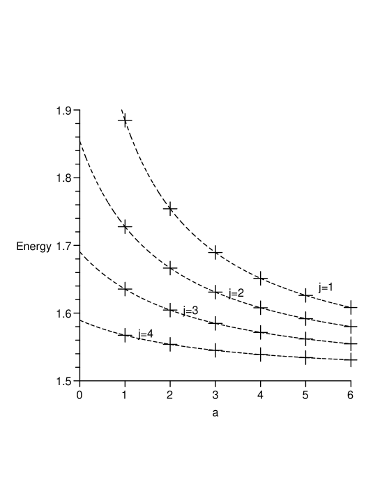
Figure 3: Energy $E-{\cal C}$ in terms of $a$ and $j$ (for $L_{0}=5$, $N=5$)

Figure 5: Vacuum state densities for $gl(5)$ spin chains with fundamental representations

Figure 6: Vacuum state densities for $gl(5)$ alternating $(a,1)-(a,3)$ spin chains

References

- [1] H. Bethe, Zur Theorie der Metalle. Eigenwerte und Eigenfunktionen Atomkete, Zeitschrift für Physik 71 (1931) 205.
- [2] W. Heisenberg, Zur Theorie der Ferromagnetismus, Zeitschrift für Physik 49 (1928) 619.
-
[3]
L.D. Faddeev and L.A. Takhtajan,
Spectrum and scattering of excitations in the one-dimensional
isotropic Heisenberg model, J. Sov. Math. 24 (1984) 241;
L.D. Faddeev and L.A. Takhtajan, What is the spin of a spin wave? Phys. Lett. A85 (1981) 375. - [4] V.E. Korepin, New effects in the massive Thirring model: repulsive case, Commun. Math. Phys. 76 (1980) 165.
- [5] V.E. Korepin, G. Izergin and N.M. Bogoliubov, Quantum inverse scattering method, correlation functions and algebraic Bethe Ansatz (Cambridge University Press, 1993).
- [6] A.B. Zamolodchikov and V.A. Fateev, An integrable spin-1 Heisenberg chain, Sov. J. Nucl. Phys. 32 (1980) 298.
- [7] L. Mezincescu, R.I. Nepomechie and V. Rittenberg, Bethe Ansatz solution of the Fateev-Zamolodchikov quantum spin chain with boundary terms, Phys. Lett. A147 (1990) 70.
- [8] H.J. de Vega and F. Woynarovich, New Integrable Quantum Chains combining different kind of spins, J. Phys. A25 (1992) 4499.
-
[9]
S.R. Aladim and M.J. Martins,
Critical behaviour of integrable mixed-spin chains,
J. Phys. A26 (1993) L529;
M.J. Martins, The effects of a magnetic field in an integrable Heisenberg chain with mixed spins, J. Phys. A26 (1993) 7301;
S.R. Aladim and M.J. Martins, The class of universality of integrable and isotropic GL(N) mixed magnets, J. Phys. A26 (1993) 7287 and hep-th/9306049. - [10] J. Abad and M. Rios, Integrable spin chain combining different representations, cond-mat/9706136.
- [11] A. Doikou, The XXX spin quantum chain and the alternating , chain with boundaries, Nucl. Phys. B634 (2002) 591 and hep-th/0201008.
- [12] P.P. Kulish, N.Yu. Reshetikhin and E.K. Sklyanin, Yang-Baxter equation and representation theory: I, Lett. Math. Phys. 5 (1981) 393.
- [13] L.A. Takhtajan, The picture of low-lying excitations in the isotropic Heisenberg chain of arbitrary spins, Phys. Lett. A87 (1982) 479.
- [14] H.M. Babujian, Exact solution of the isotropic Heisenberg chain with arbitrary spins: thermodynamics of the model, Nucl. Phys. B215 (1983) 317.
- [15] E. Ogievetsky and P. Wiegmann, Factorized S-matrix and the Bethe Ansatz for simple Lie groups, Phys. Lett. 168B (1986) 360.
- [16] L.D. Faddeev, How Algebraic Bethe Ansatz works for integrable model, Les Houches summerschool 1995 and hep-th/9605187.
- [17] A. Kuniba and J. Suzuki, Analytic Bethe Ansatz for fundamental representations of Yangians, Commun. Math. Phys. 173 (1995) 225.
- [18] A.G. Bytsko, On integrable Hamiltonians for higher spin XXZ chain, J. Math. Phys. 44 (2003) 3698 and hep-th/0112163.
- [19] Z. Tsuboi , From the quantum Jacobi–Trudi and Giambelli formula to a nonlinear integral equation for thermodynamics of the higher spin Heisenberg model, J. Phys. A37 (2004) 1747 and cond-mat/0308333.
- [20] M. Gaudin, La fonction d’onde de Bethe, Phys. Rev. A4 (1971) 386.
- [21] I.V. Cherednik, Factorizing particles on a half line and root systems, Theor. Math. Phys. 61 (1984) 977.
- [22] E.K. Sklyanin, Boundary conditions for integrable quantum systems, J. Phys. A21 (1988) 2375.
- [23] F.C. Alcaraz, M.N. Barber, M.T. Batchelor, R.J. Baxter and G.R.W. Quispel, Surface exponents of the quantum XXZ, Ashkin–Teller and Potts models, J. Phys. A20 (1987) 6397.
- [24] N. Andrei and H. Johannesson, Heisenberg chain with impurities (an integrable model), Phys. Lett. A100 (1984) 108.
- [25] T. Fukui and N. Kawakami, Spin chains with periodic array of impurities, Phys. Rev. B55 (1997) R14709 and cond-mat/9704072.
- [26] Yupeng Wang, Exact solution of the open Heisenberg chain with two impurities, Phys. Rev. B56 (1997) 14045 and cond-mat/9805253.
- [27] D. Arnaudon, N. Crampé, A. Doikou, L. Frappat and É. Ragoucy, Analytical Bethe Ansatz for closed and open -spin chains in any representation, JSTAT 02 (2005) P02007, math-ph/0411021.
- [28] C.N. Yang, Some exact results for the many-body problem in one dimension with repulsive delta-function interaction, Rev. Lett. 19 (1967) 1312.
-
[29]
R.J. Baxter,
Partition function of the eight-vertex lattice model,
Ann. Phys. 70 (1972) 193;
J. Stat. Phys. 8 (1973) 25;
Exactly solved models in statistical mechanics (Academic Press, 1982). - [30] J.B. McGuire, Study of exactly soluble one-dimensional -body problems, J. Math. Phys. 5 (1964) 622.
- [31] A. B. Zamolodchikov and A. B. Zamolodchikov, Factorized S-matrices in two dimensions as the exact solutions of certain relativistic quantum field theory models, Annals Phys. 120 (1979) 253.
-
[32]
V.G. Drinfel’d,
Hopf algebras and the quantum Yang–Baxter
equation, Soviet. Math. Dokl. 32 (1985) 254;
A new realization of Yangians and quantized affine algebras, Soviet. Math. Dokl. 36 (1988) 212. - [33] L.D. Faddeev, N.Yu. Reshetikhin and L.A. Takhtajan, Quantization of Lie groups and Lie algebras, Leningrad Math. J. 1 (1990) 193.
- [34] A. Molev, M. Nazarov and G. Olshanski, Yangians and classical Lie algebras, Russian Math. Survey 51 (1996) 205 and hep-th/9409025.
- [35] P. Kulish and N. Yu. Reshetikhin, Diagonalisation of invariant transfer matrices and quantum N-wave system (Lee model), J. Phys. A16 (1983) L591.
- [36] W. Marshall, Antiferromagnetism, Proc. Royal Soc. (London) A232 (1955) 48.
- [37] E.H. Lieb and D.C. Mattis, Ordering energy levels of interacting spin systems, J. Math. Phys. 3 (1962) 749.
- [38] B. Sutherland, Model for a multicomponent quantum system, Phys. Rev. B12 (1975) 3795.
- [39] I.S. Gradshteyn and I.M. Ryzhik, Table of integrals, series, and products, Academic Press, Orlando, FL (1980), relation (3.231.5).